It is often convenient to treat a matrix or vector as a collection of individual blocks. For example, in step-20 (and other tutorial programs), we want to consider the global linear system in the form
-It is often convenient to treat a matrix or vector as a collection of individual blocks. For example, in step-20 (and other tutorial programs), we want to consider the global linear system in the form
+
+ \end{eqnarray*}" src="form_92.png"/>
-
where are the values of velocity and pressure degrees of freedom, respectively, is the mass matrix on the velocity space, corresponds to the negative divergence operator, and is its transpose and corresponds to the negative gradient.
+
where are the values of velocity and pressure degrees of freedom, respectively, is the mass matrix on the velocity space, corresponds to the negative divergence operator, and is its transpose and corresponds to the negative gradient.
Using such a decomposition into blocks, one can then define preconditioners that are based on the individual operators that are present in a system of equations (for example the Schur complement, in the case of step-20), rather than the entire matrix. In essence, blocks are used to reflect the structure of a PDE system in linear algebra, in particular allowing for modular solvers for problems with multiple solution components. On the other hand, the matrix and right hand side vector can also treated as a unit, which is convenient for example during assembly of the linear system when one may not want to make a distinction between the individual components, or for an outer Krylov space solver that doesn't care about the block structure (e.g. if only the preconditioner needs the block structure).
Splitting matrices and vectors into blocks is supported by the BlockSparseMatrix, BlockVector, and related classes. See the overview of the various linear algebra classes in the Linear algebra classes module. The objects present two interfaces: one that makes the object look like a matrix or vector with global indexing operations, and one that makes the object look like a collection of sub-blocks that can be individually addressed. Depending on context, one may wish to use one or the other interface.
Typically, one defines the sub-structure of a matrix or vector by grouping the degrees of freedom that make up groups of physical quantities (for example all velocities) into individual blocks of the linear system. This is defined in more detail below in the glossary entry on Block (finite element).
With the exception of the number of blocks, the two objects are the same for all practical purposes, however.
Global degrees of freedom: While we have defined blocks above in terms of the vector components of a vector-valued solution function (or, equivalently, in terms of the vector-valued finite element space), every shape function of a finite element is part of one block or another. Consequently, we can partition all degrees of freedom defined on a DoFHandler into individual blocks. Since by default the DoFHandler class enumerates degrees of freedom in a more or less random way, you will first want to call the DoFRenumbering::component_wise function to make sure that all degrees of freedom that correspond to a single block are enumerated consecutively.
-
If you do this, you naturally partition matrices and vectors into blocks as well (see block (linear algebra)). In most cases, when you subdivide a matrix or vector into blocks, you do so by creating one block for each block defined by the finite element (i.e. in most practical cases the FESystem object). However, this needs not be so: the DoFRenumbering::component_wise function allows to group several vector components or finite element blocks into the same logical block (see, for example, the step-22 or step-31 tutorial programs, as opposed to step-20). As a consequence, using this feature, we can achieve the same result, i.e. subdividing matrices into blocks and vectors into 2 blocks, for the second way of creating a Stokes element outlined above using an extra argument as we would have using the first way of creating the Stokes element with two blocks right away.
+
If you do this, you naturally partition matrices and vectors into blocks as well (see block (linear algebra)). In most cases, when you subdivide a matrix or vector into blocks, you do so by creating one block for each block defined by the finite element (i.e. in most practical cases the FESystem object). However, this needs not be so: the DoFRenumbering::component_wise function allows to group several vector components or finite element blocks into the same logical block (see, for example, the step-22 or step-31 tutorial programs, as opposed to step-20). As a consequence, using this feature, we can achieve the same result, i.e. subdividing matrices into blocks and vectors into 2 blocks, for the second way of creating a Stokes element outlined above using an extra argument as we would have using the first way of creating the Stokes element with two blocks right away.
More information on this topic can be found in the documentation of FESystem, the Handling vector valued problems module and the tutorial programs referenced therein.
Selecting blocks: Many functions allow you to restrict their operation to certain vector components or blocks. For example, this is the case for the functions that interpolate boundary values: one may want to only interpolate the boundary values for the velocity block of a finite element field but not the pressure block. The way to do this is by passing a BlockMask argument to such functions, see the block mask entry of this glossary.
@@ -162,14 +162,14 @@
Boundary form
For a dim-dimensional triangulation in dim-dimensional space, the boundary form is a vector defined on faces. It is the vector product of the image of coordinate vectors on the surface of the unit cell. It is a vector normal to the surface, pointing outwards and having the length of the surface element.
-
A more general definition would be that (at least up to the length of this vector) it is exactly that vector that is necessary when considering integration by parts, i.e. equalities of the form . Using this definition then also explains what this vector should be in the case of domains (and corresponding triangulations) of dimension dim that are embedded in a space spacedim: in that case, the boundary form is still a vector defined on the faces of the triangulation; it is orthogonal to all tangent directions of the boundary and within the tangent plane of the domain. Note that this is compatible with case dim==spacedim since there the tangent plane is the entire space .
+
A more general definition would be that (at least up to the length of this vector) it is exactly that vector that is necessary when considering integration by parts, i.e. equalities of the form . Using this definition then also explains what this vector should be in the case of domains (and corresponding triangulations) of dimension dim that are embedded in a space spacedim: in that case, the boundary form is still a vector defined on the faces of the triangulation; it is orthogonal to all tangent directions of the boundary and within the tangent plane of the domain. Note that this is compatible with case dim==spacedim since there the tangent plane is the entire space .
In either case, the length of the vector equals the determinant of the transformation of reference face to the face of the current cell.
Boundary indicator
In a Triangulation object, every part of the boundary may be associated with a unique number (of type types::boundary_id) that is used to determine what kinds of boundary conditions are to be applied to a particular part of a boundary. The boundary is composed of the faces of the cells and, in 3d, the edges of these faces.
-
By default, all boundary indicators of a mesh are zero, unless you are reading from a mesh file that specifically sets them to something different, or unless you use one of the mesh generation functions in namespace GridGenerator that have a colorize option. A typical piece of code that sets the boundary indicator on part of the boundary to something else would look like this, here setting the boundary indicator to 42 for all faces located at :
for (auto &face : triangulation.active_face_iterators())
+
By default, all boundary indicators of a mesh are zero, unless you are reading from a mesh file that specifically sets them to something different, or unless you use one of the mesh generation functions in namespace GridGenerator that have a colorize option. A typical piece of code that sets the boundary indicator on part of the boundary to something else would look like this, here setting the boundary indicator to 42 for all faces located at :
for (auto &face : triangulation.active_face_iterators())
if (face->at_boundary())
if (face->center()[0] == -1)
face->set_boundary_id (42);
@@ -237,7 +237,7 @@
Component
-
When considering systems of equations in which the solution is not just a single scalar function, we say that we have a vector system with a vector-valued solution. For example, the vector solution in the elasticity equation considered in step-8 is consisting of the displacements in each of the three coordinate directions. The solution then has three elements. Similarly, the 3d Stokes equation considered in step-22 has four elements: . We call the elements of the vector-valued solution components in deal.II. To be well-posed, for the solution to have components, there need to be partial differential equations to describe them. This concept is discussed in great detail in the Handling vector valued problems module.
+
When considering systems of equations in which the solution is not just a single scalar function, we say that we have a vector system with a vector-valued solution. For example, the vector solution in the elasticity equation considered in step-8 is consisting of the displacements in each of the three coordinate directions. The solution then has three elements. Similarly, the 3d Stokes equation considered in step-22 has four elements: . We call the elements of the vector-valued solution components in deal.II. To be well-posed, for the solution to have components, there need to be partial differential equations to describe them. This concept is discussed in great detail in the Handling vector valued problems module.
In finite element programs, one frequently wants to address individual elements (components) of this vector-valued solution, or sets of components. For example, we do this extensively in step-8, and a lot of documentation is also provided in the module on Handling vector valued problems. If you are thinking only in terms of the partial differential equation (not in terms of its discretization), then the concept of components is the natural one.
On the other hand, when talking about finite elements and degrees of freedom, components are not always the correct concept because components are not always individually addressable. In particular, this is the case for non-primitive finite elements. Similarly, one may not always want to address individual components but rather sets of components — e.g. all velocity components together, and separate from the pressure in the Stokes system, without further splitting the velocities into their individual components. In either case, the correct concept to think in is that of a block. Since each component, if individually addressable, is also a block, thinking in terms of blocks is most frequently the better strategy.
would result in a mask [true, true, false] in 2d. Of course, in 3d, the result would be [true, true, true, false].
Note
Just as one can think of composed elements as being made up of components or blocks, there are component masks (represented by the ComponentMask class) and block masks (represented by the BlockMask class). The FiniteElement class has functions that convert between the two kinds of objects.
-Not all component masks actually make sense. For example, if you have a FE_RaviartThomas object in 2d, then it doesn't make any sense to have a component mask of the form [true, false] because you try to select individual vector components of a finite element where each shape function has both and velocities. In essence, while you can of course create such a component mask, there is nothing you can do with it.
+Not all component masks actually make sense. For example, if you have a FE_RaviartThomas object in 2d, then it doesn't make any sense to have a component mask of the form [true, false] because you try to select individual vector components of a finite element where each shape function has both and velocities. In essence, while you can of course create such a component mask, there is nothing you can do with it.
Compressing distributed vectors and matrices
For parallel computations, deal.II uses the vector and matrix classes defined in the PETScWrappers and TrilinosWrappers namespaces. When running programs in parallel using MPI, these classes only store a certain number of rows or elements on the current processor, whereas the rest of the vector or matrix is stored on the other processors that belong to our MPI universe. This presents a certain problem when you assemble linear systems: we add elements to the matrix and right hand side vectors that may or may not be stored locally. Sometimes, we may also want to just set an element, not add to it.
@@ -301,9 +301,9 @@
Degree of freedom
-
The term "degree of freedom" (often abbreviated as "DoF") is commonly used in the finite element community to indicate two slightly different, but related things. The first is that we'd like to represent the finite element solution as a linear combination of shape functions, in the form . Here, is a vector of expansion coefficients. Because we don't know their values yet (we will compute them as the solution of a linear or nonlinear system), they are called "unknowns" or "degrees of freedom". The second meaning of the term can be explained as follows: A mathematical description of finite element problem is often to say that we are looking for a finite dimensional function that satisfies some set of equations (e.g. for all test functions ). In other words, all we say here that the solution needs to lie in some space . However, to actually solve this problem on a computer we need to choose a basis of this space; this is the set of shape functions we have used above in the expansion of with coefficients . There are of course many bases of the space , but we will specifically choose the one that is described by the finite element functions that are traditionally defined locally on the cells of the mesh. Describing "degrees of freedom" in this context requires us to simply enumerate the basis functions of the space . For elements this means simply enumerating the vertices of the mesh in some way, but for higher elements one also has to enumerate the shape functions that are associated with edges, faces, or cell interiors of the mesh. The class that provides this enumeration of the basis functions of is called DoFHandler. The process of enumerating degrees of freedom is referred to as "distributing DoFs" in deal.II.
+
The term "degree of freedom" (often abbreviated as "DoF") is commonly used in the finite element community to indicate two slightly different, but related things. The first is that we'd like to represent the finite element solution as a linear combination of shape functions, in the form . Here, is a vector of expansion coefficients. Because we don't know their values yet (we will compute them as the solution of a linear or nonlinear system), they are called "unknowns" or "degrees of freedom". The second meaning of the term can be explained as follows: A mathematical description of finite element problem is often to say that we are looking for a finite dimensional function that satisfies some set of equations (e.g. for all test functions ). In other words, all we say here that the solution needs to lie in some space . However, to actually solve this problem on a computer we need to choose a basis of this space; this is the set of shape functions we have used above in the expansion of with coefficients . There are of course many bases of the space , but we will specifically choose the one that is described by the finite element functions that are traditionally defined locally on the cells of the mesh. Describing "degrees of freedom" in this context requires us to simply enumerate the basis functions of the space . For elements this means simply enumerating the vertices of the mesh in some way, but for higher elements one also has to enumerate the shape functions that are associated with edges, faces, or cell interiors of the mesh. The class that provides this enumeration of the basis functions of is called DoFHandler. The process of enumerating degrees of freedom is referred to as "distributing DoFs" in deal.II.
Direction flags
@@ -324,7 +324,7 @@
Distorted cells
A distorted cell is a cell for which the mapping from the reference cell to real cell has a Jacobian whose determinant is non-positive somewhere in the cell. Typically, we only check the sign of this determinant at the vertices of the cell. The function GeometryInfo::alternating_form_at_vertices computes these determinants at the vertices.
-
By way of example, if all of the determinants are of roughly equal value and on the order of then the cell is well-shaped. For example, a square cell or face has determinants equal to whereas a strongly sheared parallelogram has a determinant much smaller. Similarly, a cell with very unequal edge lengths will have widely varying determinants. Conversely, a pinched cell in which the location of two or more vertices is collapsed to a single point has a zero determinant at this location. Finally, an inverted or twisted cell in which the location of two vertices is out of order will have negative determinants.
+
By way of example, if all of the determinants are of roughly equal value and on the order of then the cell is well-shaped. For example, a square cell or face has determinants equal to whereas a strongly sheared parallelogram has a determinant much smaller. Similarly, a cell with very unequal edge lengths will have widely varying determinants. Conversely, a pinched cell in which the location of two or more vertices is collapsed to a single point has a zero determinant at this location. Finally, an inverted or twisted cell in which the location of two vertices is out of order will have negative determinants.
The following two images show a well-formed, a pinched, and a twisted cell for both 2d and 3d:
@@ -363,19 +363,19 @@
Generalized support points
-
"Generalized support points" are, as the name suggests, a generalization of support points. The latter are used to describe that a finite element simply interpolates values at individual points (the "support points"). If we call these points (where the hat indicates that these points are defined on the reference cell ), then one typically defines shape functions in such a way that the nodal functionals simply evaluate the function at the support point, i.e., that , and the basis is chosen so that where is the Kronecker delta function. This leads to the common Lagrange elements.
-
(In the vector valued case, the only other piece of information besides the support points that one needs to provide is the vector component the th node functional corresponds, so that .)
-
On the other hand, there are other kinds of elements that are not defined this way. For example, for the lowest order Raviart-Thomas element (see the FE_RaviartThomas class), the node functional evaluates not individual components of a vector-valued finite element function with dim components, but the normal component of this vector: "Generalized support points" are, as the name suggests, a generalization of support points. The latter are used to describe that a finite element simply interpolates values at individual points (the "support points"). If we call these points (where the hat indicates that these points are defined on the reference cell ), then one typically defines shape functions in such a way that the nodal functionals simply evaluate the function at the support point, i.e., that , and the basis is chosen so that where is the Kronecker delta function. This leads to the common Lagrange elements.
+
(In the vector valued case, the only other piece of information besides the support points that one needs to provide is the vector component the th node functional corresponds, so that .)
+
On the other hand, there are other kinds of elements that are not defined this way. For example, for the lowest order Raviart-Thomas element (see the FE_RaviartThomas class), the node functional evaluates not individual components of a vector-valued finite element function with dim components, but the normal component of this vector: , where the are the normal vectors to the face of the cell on which is located. In other words, the node functional is a linear combination of the components of when evaluated at . Similar things happen for the BDM, ABF, and Nedelec elements (see the FE_BDM, FE_ABF, FE_Nedelec classes).
-
In these cases, the element does not have support points because it is not purely interpolatory; however, some kind of interpolation is still involved when defining shape functions as the node functionals still require point evaluations at special points . In these cases, we call the points generalized support points.
-
Finally, there are elements that still do not fit into this scheme. For example, some hierarchical basis functions (see, for example the FE_Q_Hierarchical element) are defined so that the node functionals are moments of finite element functions, , where the are the normal vectors to the face of the cell on which is located. In other words, the node functional is a linear combination of the components of when evaluated at . Similar things happen for the BDM, ABF, and Nedelec elements (see the FE_BDM, FE_ABF, FE_Nedelec classes).
+
In these cases, the element does not have support points because it is not purely interpolatory; however, some kind of interpolation is still involved when defining shape functions as the node functionals still require point evaluations at special points . In these cases, we call the points generalized support points.
+
Finally, there are elements that still do not fit into this scheme. For example, some hierarchical basis functions (see, for example the FE_Q_Hierarchical element) are defined so that the node functionals are moments of finite element functions, in 2d, and similarly for 3d, where the are the order of the moment described by shape function . Some other elements use moments over edges or faces. In all of these cases, node functionals are not defined through interpolation at all, and these elements then have neither support points, nor generalized support points.
+ $" src="form_124.png"/> in 2d, and similarly for 3d, where the are the order of the moment described by shape function . Some other elements use moments over edges or faces. In all of these cases, node functionals are not defined through interpolation at all, and these elements then have neither support points, nor generalized support points.
The numerical examples shown in that paper are generated with a slightly modified version of step-27. The main difference to that tutorial program is that various operations in the program were timed for the paper to compare different options and show that methods are really not all that expensive.
+
The numerical examples shown in that paper are generated with a slightly modified version of step-27. The main difference to that tutorial program is that various operations in the program were timed for the paper to compare different options and show that methods are really not all that expensive.
It frequently appears in the solution of time dependent problems where, if one uses an explicit time stepping method, it then leads to the need to solve problems of the form
-
+ \end{align*}" src="form_127.png"/>
-
in time step , where is the solution to be computed, is the known solution from the first time step, and is a matrix related to the differential operator in the PDE. is the size of the time step. A similar linear system of equations also arises out of the discretization of second-order differential equations.
-
The presence of the matrix on the left side is a nuisance because, even though we have used an explicit time stepping method, we still have to solve a linear system in each time step. It would be much preferable if the matrix were diagonal. "Lumping" the mass matrix is a strategy to replace by a matrix that actually is diagonal, yet does not destroy the accuracy of the resulting solution.
-
Historically, mass lumping was performed by adding the elements of a row together and setting the diagonal entries of to that sum. This works for and elements, for example, and can be understood mechanically by replacing the continuous medium we are discretizating by one where the continuous mass distribution is replaced by one where (finite amounts of) mass are located only at the nodes. That is, we are "lumping together" the mass of an element at its vertices, thus giving rise to the name "lumped mass matrix". A more mathematical perspective is to compute the integral above for via special quadrature rules; in particular, we replace the computation of
-, where is the solution to be computed, is the known solution from the first time step, and is a matrix related to the differential operator in the PDE. is the size of the time step. A similar linear system of equations also arises out of the discretization of second-order differential equations.
+
The presence of the matrix on the left side is a nuisance because, even though we have used an explicit time stepping method, we still have to solve a linear system in each time step. It would be much preferable if the matrix were diagonal. "Lumping" the mass matrix is a strategy to replace by a matrix that actually is diagonal, yet does not destroy the accuracy of the resulting solution.
+
Historically, mass lumping was performed by adding the elements of a row together and setting the diagonal entries of to that sum. This works for and elements, for example, and can be understood mechanically by replacing the continuous medium we are discretizating by one where the continuous mass distribution is replaced by one where (finite amounts of) mass are located only at the nodes. That is, we are "lumping together" the mass of an element at its vertices, thus giving rise to the name "lumped mass matrix". A more mathematical perspective is to compute the integral above for via special quadrature rules; in particular, we replace the computation of
+
+ \end{align*}" src="form_134.png"/>
by quadrature
-
+ \end{align*}" src="form_135.png"/>
where we choose the quadrature points as the nodes at which the shape functions are defined. If we order the quadrature points in the same way as the shape functions, then
-
+ \end{align*}" src="form_136.png"/>
and consequently
-
+ \end{align*}" src="form_137.png"/>
-
where the sum extends over those cells on which is nonzero. The so-computed mass matrix is therefore diagonal.
-
Whether or not this particular choice of quadrature formula is sufficient to retain the convergence rate of the discretization is a separate question. For the usual finite elements (implemented by FE_Q and FE_DGQ), the appropriate quadrature formulas are of QGaussLobatto type. Mass lumping can also be done with FE_SimplexP_Bubbles, for example, if appropriate quadrature rules are chosen.
+
where the sum extends over those cells on which is nonzero. The so-computed mass matrix is therefore diagonal.
+
Whether or not this particular choice of quadrature formula is sufficient to retain the convergence rate of the discretization is a separate question. For the usual finite elements (implemented by FE_Q and FE_DGQ), the appropriate quadrature formulas are of QGaussLobatto type. Mass lumping can also be done with FE_SimplexP_Bubbles, for example, if appropriate quadrature rules are chosen.
For an example of where lumped mass matrices play a role, see step-69.
Manifold indicator
Every object that makes up a Triangulation (cells, faces, edges, etc.), is associated with a unique number (of type types::manifold_id) that is used to identify which manifold object is responsible to generate new points when the mesh is refined.
-
By default, all manifold indicators of a mesh are set to numbers::flat_manifold_id. A typical piece of code that sets the manifold indicator on a object to something else would look like this, here setting the manifold indicator to 42 for all cells whose center has an component less than zero:
+
By default, all manifold indicators of a mesh are set to numbers::flat_manifold_id. A typical piece of code that sets the manifold indicator on a object to something else would look like this, here setting the manifold indicator to 42 for all cells whose center has an component less than zero:
for (auto &cell : triangulation.active_cell_iterators())
Improved: The FEValuesViews objects that one gets when writing things like fe_values[velocities] (see Handling vector valued problems) have become a lot smarter. They now compute a significant amount of data at creation time, rather than on the fly. This means that creating such objects becomes more expensive but using them is cheaper. To offset this cost, FEValuesBase objects now create all possible FEValuesViews objects at creation time, rather than whenever you do things like fe_values[velocities], and simply return a reference to a pre-generated object. This turns an effort into an effort, where is the number of cells.
+
Improved: The FEValuesViews objects that one gets when writing things like fe_values[velocities] (see Handling vector valued problems) have become a lot smarter. They now compute a significant amount of data at creation time, rather than on the fly. This means that creating such objects becomes more expensive but using them is cheaper. To offset this cost, FEValuesBase objects now create all possible FEValuesViews objects at creation time, rather than whenever you do things like fe_values[velocities], and simply return a reference to a pre-generated object. This turns an effort into an effort, where is the number of cells.
(WB 2008/12/10)
/usr/share/doc/packages/dealii-openmpi4/doxygen/deal.II/changes_between_6_2_and_6_3.html differs (JavaScript source, ASCII text, with very long lines (994))
--- old//usr/share/doc/packages/dealii-openmpi4/doxygen/deal.II/changes_between_6_2_and_6_3.html 2023-11-25 15:25:50.673410996 +0100
+++ new//usr/share/doc/packages/dealii-openmpi4/doxygen/deal.II/changes_between_6_2_and_6_3.html 2023-11-25 15:25:50.673410996 +0100
@@ -364,7 +364,7 @@
/usr/share/doc/packages/dealii-openmpi4/doxygen/deal.II/changes_between_7_0_and_7_1.html differs (JavaScript source, ASCII text, with very long lines (1392))
--- old//usr/share/doc/packages/dealii-openmpi4/doxygen/deal.II/changes_between_7_0_and_7_1.html 2023-11-25 15:25:50.686744058 +0100
+++ new//usr/share/doc/packages/dealii-openmpi4/doxygen/deal.II/changes_between_7_0_and_7_1.html 2023-11-25 15:25:50.686744058 +0100
@@ -374,7 +374,7 @@
-
Improved: Evaluation of Lagrangian basis functions has been made stable by exchanging polynomial evaluation from the standard form to a product of linear factors, . This ensures accurate evaluation up to very high order and avoids inaccuracies when using high order finite elements.
+
Improved: Evaluation of Lagrangian basis functions has been made stable by exchanging polynomial evaluation from the standard form to a product of linear factors, . This ensures accurate evaluation up to very high order and avoids inaccuracies when using high order finite elements.
(Martin Kronbichler 2011/07/26)
/usr/share/doc/packages/dealii-openmpi4/doxygen/deal.II/changes_between_7_1_and_7_2.html differs (JavaScript source, ASCII text, with very long lines (1108))
--- old//usr/share/doc/packages/dealii-openmpi4/doxygen/deal.II/changes_between_7_1_and_7_2.html 2023-11-25 15:25:50.703410385 +0100
+++ new//usr/share/doc/packages/dealii-openmpi4/doxygen/deal.II/changes_between_7_1_and_7_2.html 2023-11-25 15:25:50.703410385 +0100
@@ -330,7 +330,7 @@
Fixed: Computing the norm and seminorm in VectorTools::integrate_difference was not implemented. This is now fixed.
(Wolfgang Bangerth 2012/06/02)
/usr/share/doc/packages/dealii-openmpi4/doxygen/deal.II/changes_between_8_1_and_8_2.html differs (JavaScript source, ASCII text, with very long lines (948))
--- old//usr/share/doc/packages/dealii-openmpi4/doxygen/deal.II/changes_between_8_1_and_8_2.html 2023-11-25 15:25:50.716743445 +0100
+++ new//usr/share/doc/packages/dealii-openmpi4/doxygen/deal.II/changes_between_8_1_and_8_2.html 2023-11-25 15:25:50.716743445 +0100
@@ -837,7 +837,7 @@
-
New: There is now a new class Functions::InterpolatedTensorProductGridData that can be used to (bi-/tri-)linearly interpolate data given on a tensor product mesh of (and and ) values, for example to evaluate experimentally determined coefficients, or to assess the accuracy of a solution by comparing with a solution generated by a different code and written in gridded data. There is also a new class Functions::InterpolatedUniformGridData that can perform the same task more efficiently if the data is stored on meshes that are uniform in each coordinate direction.
+
New: There is now a new class Functions::InterpolatedTensorProductGridData that can be used to (bi-/tri-)linearly interpolate data given on a tensor product mesh of (and and ) values, for example to evaluate experimentally determined coefficients, or to assess the accuracy of a solution by comparing with a solution generated by a different code and written in gridded data. There is also a new class Functions::InterpolatedUniformGridData that can perform the same task more efficiently if the data is stored on meshes that are uniform in each coordinate direction.
(Wolfgang Bangerth, 2013/12/20)
/usr/share/doc/packages/dealii-openmpi4/doxygen/deal.II/changes_between_8_4_2_and_8_5_0.html differs (JavaScript source, ASCII text, with very long lines (1360))
--- old//usr/share/doc/packages/dealii-openmpi4/doxygen/deal.II/changes_between_8_4_2_and_8_5_0.html 2023-11-25 15:25:50.736743038 +0100
+++ new//usr/share/doc/packages/dealii-openmpi4/doxygen/deal.II/changes_between_8_4_2_and_8_5_0.html 2023-11-25 15:25:50.736743038 +0100
@@ -516,7 +516,7 @@
-
Fixed: The FE_ABF class reported the maximal polynomial degree (via FiniteElement::degree) for elements of order as , but this is wrong. It should be (see Section 5 of the original paper of Arnold, Boffi, and Falk). This is now fixed.
+
Fixed: The FE_ABF class reported the maximal polynomial degree (via FiniteElement::degree) for elements of order as , but this is wrong. It should be (see Section 5 of the original paper of Arnold, Boffi, and Falk). This is now fixed.
(Wolfgang Bangerth, 2017/01/13)
/usr/share/doc/packages/dealii-openmpi4/doxygen/deal.II/changes_between_9_1_1_and_9_2_0.html differs (JavaScript source, ASCII text, with very long lines (1176))
--- old//usr/share/doc/packages/dealii-openmpi4/doxygen/deal.II/changes_between_9_1_1_and_9_2_0.html 2023-11-25 15:25:50.760075899 +0100
+++ new//usr/share/doc/packages/dealii-openmpi4/doxygen/deal.II/changes_between_9_1_1_and_9_2_0.html 2023-11-25 15:25:50.760075899 +0100
@@ -606,7 +606,7 @@
-
Improved: GridGenerator::hyper_shell() in 3d now supports more n_cells options. While previously only 6, 12, or 96 cells were possible, the function now supports any number of the kind with a non-negative integer. The new cases and correspond to refinement in the azimuthal direction of the 6 or 12 cell case with a single mesh layer in radial direction, and are intended for shells that are thin and should be given more resolution in azimuthal direction.
+
Improved: GridGenerator::hyper_shell() in 3d now supports more n_cells options. While previously only 6, 12, or 96 cells were possible, the function now supports any number of the kind with a non-negative integer. The new cases and correspond to refinement in the azimuthal direction of the 6 or 12 cell case with a single mesh layer in radial direction, and are intended for shells that are thin and should be given more resolution in azimuthal direction.
(Martin Kronbichler, 2020/04/07)
@@ -1560,7 +1560,7 @@
-
Improved: The additional roots of the HermiteLikeInterpolation with degree greater than four have been switched to the roots of the Jacobi polynomial , making the interior bubble functions orthogonal and improving the conditioning of interpolation slightly.
+
Improved: The additional roots of the HermiteLikeInterpolation with degree greater than four have been switched to the roots of the Jacobi polynomial , making the interior bubble functions orthogonal and improving the conditioning of interpolation slightly.
(Martin Kronbichler, 2019/07/12)
/usr/share/doc/packages/dealii-openmpi4/doxygen/deal.II/classAffineConstraints.html differs (JavaScript source, ASCII text, with very long lines (1132))
--- old//usr/share/doc/packages/dealii-openmpi4/doxygen/deal.II/classAffineConstraints.html 2023-11-25 15:25:50.793408553 +0100
+++ new//usr/share/doc/packages/dealii-openmpi4/doxygen/deal.II/classAffineConstraints.html 2023-11-25 15:25:50.790075289 +0100
@@ -357,9 +357,9 @@
The algorithms used in the implementation of this class are described in some detail in the hp-paper. There is also a significant amount of documentation on how to use this class in the Constraints on degrees of freedom module.
Description of constraints
Each "line" in objects of this class corresponds to one constrained degree of freedom, with the number of the line being i, entered by using add_line() or add_lines(). The entries in this line are pairs of the form (j,aij), which are added by add_entry() or add_entries(). The organization is essentially a SparsityPattern, but with only a few lines containing nonzero elements, and therefore no data wasted on the others. For each line, which has been added by the mechanism above, an elimination of the constrained degree of freedom of the form
-
+\]" src="form_1577.png"/>
is performed, where bi is optional and set by set_inhomogeneity(). Thus, if a constraint is formulated for instance as a zero mean value of several degrees of freedom, one of the degrees has to be chosen to be eliminated.
Note that the constraints are linear in the xi, and that there might be a constant (non-homogeneous) term in the constraint. This is exactly the form we need for hanging node constraints, where we need to constrain one degree of freedom in terms of others. There are other conditions of this form possible, for example for implementing mean value conditions as is done in the step-11 tutorial program. The name of the class stems from the fact that these constraints can be represented in matrix form as Xx = b, and this object then describes the matrix X and the vector b. The most frequent way to create/fill objects of this type is using the DoFTools::make_hanging_node_constraints() function. The use of these objects is first explained in step-6.
@@ -929,13 +929,13 @@
-
Add an entry to a given line. In other words, this function adds a term to the constraints for the th degree of freedom.
+
Add an entry to a given line. In other words, this function adds a term to the constraints for the th degree of freedom.
If an entry with the same indices as the one this function call denotes already exists, then this function simply returns provided that the value of the entry is the same. Thus, it does no harm to enter a constraint twice.
Parameters
-
[in]
constrained_dof_index
The index of the degree of freedom that is being constrained.
-
[in]
column
The index of the degree of freedom being entered into the constraint for degree of freedom .
-
[in]
weight
The factor that multiplies .
+
[in]
constrained_dof_index
The index of the degree of freedom that is being constrained.
+
[in]
column
The index of the degree of freedom being entered into the constraint for degree of freedom .
+
[in]
weight
The factor that multiplies .
@@ -1010,11 +1010,11 @@
-
Set an inhomogeneity to the constraint for a degree of freedom. In other words, it adds a constant to the constraint for degree of freedom . For this to work, you need to call add_line() first for the given degree of freedom.
+
Set an inhomogeneity to the constraint for a degree of freedom. In other words, it adds a constant to the constraint for degree of freedom . For this to work, you need to call add_line() first for the given degree of freedom.
Parameters
-
[in]
constrained_dof_index
The index of the degree of freedom that is being constrained.
-
[in]
value
The right hand side value for the constraint on the degree of freedom .
+
[in]
constrained_dof_index
The index of the degree of freedom that is being constrained.
+
[in]
value
The right hand side value for the constraint on the degree of freedom .
@@ -1042,9 +1042,9 @@
Close the filling of entries. Since the lines of a matrix of this type are usually filled in an arbitrary order and since we do not want to use associative constrainers to store the lines, we need to sort the lines and within the lines the columns before usage of the matrix. This is done through this function.
Also, zero entries are discarded, since they are not needed.
After closing, no more entries are accepted. If the object was already closed, then this function returns immediately.
-
This function also resolves chains of constraints. For example, degree of freedom 13 may be constrained to while degree of freedom 7 is itself constrained as . Then, the resolution will be that . Note, however, that cycles in this graph of constraints are not allowed, i.e., for example may not itself be constrained, directly or indirectly, to again.
+
This function also resolves chains of constraints. For example, degree of freedom 13 may be constrained to while degree of freedom 7 is itself constrained as . Then, the resolution will be that . Note, however, that cycles in this graph of constraints are not allowed, i.e., for example may not itself be constrained, directly or indirectly, to again.
@@ -1487,9 +1487,9 @@
Print the constraints represented by the current object to the given stream.
For each constraint of the form
-
+\]" src="form_1586.png"/>
this function will write a sequence of lines that look like this:
42 2 : 0.5
42 14 : 0.25
@@ -2150,7 +2150,7 @@
This function takes a matrix of local contributions (local_matrix) corresponding to the degrees of freedom indices given in local_dof_indices and distributes them to the global matrix. In other words, this function implements a scatter operation. In most cases, these local contributions will be the result of an integration over a cell or face of a cell. However, as long as local_matrix and local_dof_indices have the same number of elements, this function is happy with whatever it is given.
In contrast to the similar function in the DoFAccessor class, this function also takes care of constraints, i.e. if one of the elements of local_dof_indices belongs to a constrained node, then rather than writing the corresponding element of local_matrix into global_matrix, the element is distributed to the entries in the global matrix to which this particular degree of freedom is constrained.
-
With this scheme, we never write into rows or columns of constrained degrees of freedom. In order to make sure that the resulting matrix can still be inverted, we need to do something with the diagonal elements corresponding to constrained nodes. Thus, if a degree of freedom in local_dof_indices is constrained, we distribute the corresponding entries in the matrix, but also add the absolute value of the diagonal entry of the local matrix to the corresponding entry in the global matrix. Assuming the discretized operator is positive definite, this guarantees that the diagonal entry is always non-zero, positive, and of the same order of magnitude as the other entries of the matrix. On the other hand, when solving a source problem the exact value of the diagonal element is not important, since the value of the respective degree of freedom will be overwritten by the distribute() call later on anyway.
+
With this scheme, we never write into rows or columns of constrained degrees of freedom. In order to make sure that the resulting matrix can still be inverted, we need to do something with the diagonal elements corresponding to constrained nodes. Thus, if a degree of freedom in local_dof_indices is constrained, we distribute the corresponding entries in the matrix, but also add the absolute value of the diagonal entry of the local matrix to the corresponding entry in the global matrix. Assuming the discretized operator is positive definite, this guarantees that the diagonal entry is always non-zero, positive, and of the same order of magnitude as the other entries of the matrix. On the other hand, when solving a source problem the exact value of the diagonal element is not important, since the value of the respective degree of freedom will be overwritten by the distribute() call later on anyway.
Note
The procedure described above adds an unforeseeable number of artificial eigenvalues to the spectrum of the matrix. Therefore, it is recommended to use the equivalent function with two local index vectors in such a case.
By using this function to distribute local contributions to the global object, one saves the call to the condense function after the vectors and matrices are fully assembled.
Note
This function in itself is thread-safe, i.e., it works properly also when several threads call it simultaneously. However, the function call is only thread-safe if the underlying global matrix allows for simultaneous access and the access is not to rows with the same global index at the same time. This needs to be made sure from the caller's site. There is no locking mechanism inside this method to prevent data races.
@@ -2200,7 +2200,7 @@
This function does almost the same as the function above but can treat general rectangular matrices. The main difference to achieve this is that the diagonal entries in constrained rows are left untouched instead of being filled with arbitrary values.
-
Since the diagonal entries corresponding to eliminated degrees of freedom are not set, the result may have a zero eigenvalue, if applied to a square matrix. This has to be considered when solving the resulting problems. For solving a source problem , it is possible to set the diagonal entry after building the matrix by a piece of code of the form
+
Since the diagonal entries corresponding to eliminated degrees of freedom are not set, the result may have a zero eigenvalue, if applied to a square matrix. This has to be considered when solving the resulting problems. For solving a source problem , it is possible to set the diagonal entry after building the matrix by a piece of code of the form
for (unsignedint i=0;i<matrix.m();++i)
if (constraints.is_constrained(i))
matrix.diag_element(i) = 1.;
@@ -2541,7 +2541,7 @@
-
Given a vector, set all constrained degrees of freedom to values so that the constraints are satisfied. For example, if the current object stores the constraint , then this function will read the values of and from the given vector and set the element according to this constraints. Similarly, if the current object stores the constraint , then this function will set the 42nd element of the given vector to 208.
+
Given a vector, set all constrained degrees of freedom to values so that the constraints are satisfied. For example, if the current object stores the constraint , then this function will read the values of and from the given vector and set the element according to this constraints. Similarly, if the current object stores the constraint , then this function will set the 42nd element of the given vector to 208.
Note
If this function is called with a parallel vector vec, then the vector must not contain ghost elements.
/usr/share/doc/packages/dealii-openmpi4/doxygen/deal.II/classAlgorithms_1_1ThetaTimestepping.html differs (JavaScript source, Unicode text, UTF-8 text, with very long lines (950))
--- old//usr/share/doc/packages/dealii-openmpi4/doxygen/deal.II/classAlgorithms_1_1ThetaTimestepping.html 2023-11-25 15:25:50.813408145 +0100
+++ new//usr/share/doc/packages/dealii-openmpi4/doxygen/deal.II/classAlgorithms_1_1ThetaTimestepping.html 2023-11-25 15:25:50.813408145 +0100
@@ -218,9 +218,9 @@
For fixed theta, the Crank-Nicolson scheme is the only second order scheme. Nevertheless, further stability may be achieved by choosing theta larger than ½, thereby introducing a first order error term. In order to avoid a loss of convergence order, the adaptive theta scheme can be used, where theta=½+c dt.
Assume that we want to solve the equation u' + F(u) = 0 with a step size k. A step of the theta scheme can be written as
-
+\]" src="form_351.png"/>
Here, M is the mass matrix. We see, that the right hand side amounts to an explicit Euler step with modified step size in weak form (up to inversion of M). The left hand side corresponds to an implicit Euler step with modified step size (right hand side given). Thus, the implementation of the theta scheme will use two Operator objects, one for the explicit, one for the implicit part. Each of these will use its own TimestepData to account for the modified step sizes (and different times if the problem is not autonomous). Note that once the explicit part has been computed, the left hand side actually constitutes a linear or nonlinear system which has to be solved.
Now we need to study the application of the implicit and explicit operator. We assume that the pointer matrix points to the matrix created in the main program (the constructor did this for us). Here, we first get the time step size from the AnyData object that was provided as input. Then, if we are in the first step or if the timestep has changed, we fill the local matrix , such that with the given matrix , it becomes
-
+
Now we need to study the application of the implicit and explicit operator. We assume that the pointer matrix points to the matrix created in the main program (the constructor did this for us). Here, we first get the time step size from the AnyData object that was provided as input. Then, if we are in the first step or if the timestep has changed, we fill the local matrix , such that with the given matrix , it becomes
+
After we have worked off the notifications, we clear them, such that the matrix is only generated when necessary.
The operator computing the explicit part of the scheme. This will receive in its input data the value at the current time with name "Current time solution". It should obtain the current time and time step size from explicit_data().
-
Its return value is , where is the current state vector, the mass matrix, the operator in space and is the adjusted time step size .
+
Its return value is , where is the current state vector, the mass matrix, the operator in space and is the adjusted time step size .
The operator solving the implicit part of the scheme. It will receive in its input data the vector "Previous time". Information on the timestep should be obtained from implicit_data().
-
Its return value is the solution u of Mu-cF(u)=f, where f is the dual space vector found in the "Previous time" entry of the input data, M the mass matrix, F the operator in space and c is the adjusted time step size
+
Its return value is the solution u of Mu-cF(u)=f, where f is the dual space vector found in the "Previous time" entry of the input data, M the mass matrix, F the operator in space and c is the adjusted time step size
/usr/share/doc/packages/dealii-openmpi4/doxygen/deal.II/classAnisotropicPolynomials.html differs (JavaScript source, ASCII text, with very long lines (1527))
--- old//usr/share/doc/packages/dealii-openmpi4/doxygen/deal.II/classAnisotropicPolynomials.html 2023-11-25 15:25:50.833407738 +0100
+++ new//usr/share/doc/packages/dealii-openmpi4/doxygen/deal.II/classAnisotropicPolynomials.html 2023-11-25 15:25:50.833407738 +0100
@@ -153,10 +153,10 @@
Detailed Description
template<int dim>
class AnisotropicPolynomials< dim >
Anisotropic tensor product of given polynomials.
-
Given one-dimensional polynomials in -direction, in -direction, and so on, this class generates polynomials of the form . (With obvious generalization if dim is in fact only 2. If dim is in fact only 1, then the result is simply the same set of one-dimensional polynomials passed to the constructor.)
-
If the elements of each set of base polynomials are mutually orthogonal on the interval or , then the tensor product polynomials are orthogonal on or , respectively.
-
The resulting dim-dimensional tensor product polynomials are ordered as follows: We iterate over the coordinates running fastest, then the coordinate, etc. For example, for dim==2, the first few polynomials are thus , , , ..., , , , etc.
+
Given one-dimensional polynomials in -direction, in -direction, and so on, this class generates polynomials of the form . (With obvious generalization if dim is in fact only 2. If dim is in fact only 1, then the result is simply the same set of one-dimensional polynomials passed to the constructor.)
+
If the elements of each set of base polynomials are mutually orthogonal on the interval or , then the tensor product polynomials are orthogonal on or , respectively.
+
The resulting dim-dimensional tensor product polynomials are ordered as follows: We iterate over the coordinates running fastest, then the coordinate, etc. For example, for dim==2, the first few polynomials are thus , , , ..., , , , etc.
Each tensor product polynomial is a product of one-dimensional polynomials in each space direction. Compute the indices of these one- dimensional polynomials for each space direction, given the index i.
+
Each tensor product polynomial is a product of one-dimensional polynomials in each space direction. Compute the indices of these one- dimensional polynomials for each space direction, given the index i.
/usr/share/doc/packages/dealii-openmpi4/doxygen/deal.II/classArpackSolver.html differs (JavaScript source, ASCII text, with very long lines (1026))
--- old//usr/share/doc/packages/dealii-openmpi4/doxygen/deal.II/classArpackSolver.html 2023-11-25 15:25:50.850074067 +0100
+++ new//usr/share/doc/packages/dealii-openmpi4/doxygen/deal.II/classArpackSolver.html 2023-11-25 15:25:50.850074067 +0100
@@ -229,14 +229,14 @@
Detailed Description
Interface for using ARPACK. ARPACK is a collection of Fortran77 subroutines designed to solve large scale eigenvalue problems. Here we interface to the routines dnaupd and dneupd of ARPACK. If the operator is specified to be symmetric we use the symmetric interface dsaupd and dseupd of ARPACK instead. The package is designed to compute a few eigenvalues and corresponding eigenvectors of a general n by n matrix A. It is most appropriate for large sparse matrices A.
-
In this class we make use of the method applied to the generalized eigenspectrum problem , for ; where is a system matrix, is a mass matrix, and are a set of eigenvalues and eigenvectors respectively.
+
In this class we make use of the method applied to the generalized eigenspectrum problem , for ; where is a system matrix, is a mass matrix, and are a set of eigenvalues and eigenvectors respectively.
The ArpackSolver can be used in application codes with serial objects in the following way:
for the generalized eigenvalue problem , where the variable size_of_spectrum tells ARPACK the number of eigenvector/eigenvalue pairs to solve for. Here, lambda is a vector that will contain the eigenvalues computed, x a vector that will contain the eigenvectors computed, and OP is an inverse operation for the matrix A. Shift and invert transformation around zero is applied.
+
for the generalized eigenvalue problem , where the variable size_of_spectrum tells ARPACK the number of eigenvector/eigenvalue pairs to solve for. Here, lambda is a vector that will contain the eigenvalues computed, x a vector that will contain the eigenvectors computed, and OP is an inverse operation for the matrix A. Shift and invert transformation around zero is applied.
Through the AdditionalData the user can specify some of the parameters to be set.
For further information on how the ARPACK routines dsaupd, dseupd, dnaupd and dneupd work and also how to set the parameters appropriately please take a look into the ARPACK manual.
Note
Whenever you eliminate degrees of freedom using AffineConstraints, you generate spurious eigenvalues and eigenvectors. If you make sure that the diagonals of eliminated matrix rows are all equal to one, you get a single additional eigenvalue. But beware that some functions in deal.II set these diagonals to rather arbitrary (from the point of view of eigenvalue problems) values. See also step-36 for an example.
@@ -525,7 +525,7 @@
-
Solve the generalized eigensprectrum problem by calling the dsaupd and dseupd or dnaupd and dneupd functions of ARPACK.
+
Solve the generalized eigensprectrum problem by calling the dsaupd and dseupd or dnaupd and dneupd functions of ARPACK.
The function returns a vector of eigenvalues of length n and a vector of eigenvectors of length n in the symmetric case and of length n+1 in the non-symmetric case. In the symmetric case all eigenvectors are real. In the non-symmetric case complex eigenvalues always occur as complex conjugate pairs. Therefore the eigenvector for an eigenvalue with nonzero complex part is stored by putting the real and the imaginary parts in consecutive real-valued vectors. The eigenvector of the complex conjugate eigenvalue does not need to be stored, since it is just the complex conjugate of the stored eigenvector. Thus, if the last n-th eigenvalue has a nonzero imaginary part, Arpack needs in total n+1 real-valued vectors to store real and imaginary parts of the eigenvectors.
Parameters
/usr/share/doc/packages/dealii-openmpi4/doxygen/deal.II/classArrayView.html differs (JavaScript source, ASCII text, with very long lines (911))
--- old//usr/share/doc/packages/dealii-openmpi4/doxygen/deal.II/classArrayView.html 2023-11-25 15:25:50.873406924 +0100
+++ new//usr/share/doc/packages/dealii-openmpi4/doxygen/deal.II/classArrayView.html 2023-11-25 15:25:50.873406924 +0100
@@ -1025,7 +1025,7 @@
-
Return a reference to the th element of the range represented by the current object.
+
Return a reference to the th element of the range represented by the current object.
This function is marked as const because it does not change the view object. It may however return a reference to a non-const memory location depending on whether the template type of the class is const or not.
This function is only allowed to be called if the underlying data is indeed stored in CPU memory.
/usr/share/doc/packages/dealii-openmpi4/doxygen/deal.II/classAutoDerivativeFunction.html differs (JavaScript source, ASCII text, with very long lines (2139))
--- old//usr/share/doc/packages/dealii-openmpi4/doxygen/deal.II/classAutoDerivativeFunction.html 2023-11-25 15:25:50.896739784 +0100
+++ new//usr/share/doc/packages/dealii-openmpi4/doxygen/deal.II/classAutoDerivativeFunction.html 2023-11-25 15:25:50.896739784 +0100
@@ -346,27 +346,27 @@
where each value is the relative weight of each vertex (so the centroid is, in 2d, where each ). Since we only consider convex combinations we can rewrite this equation as
+
where each value is the relative weight of each vertex (so the centroid is, in 2d, where each ). Since we only consider convex combinations we can rewrite this equation as
Detailed Description
template<typename VectorType>
class BaseQR< VectorType >
This class and classes derived from it are meant to build and matrices one row/column at a time, i.e., by growing matrix from an empty matrix to , where is the number of added column vectors.
-
As a consequence, matrices which have the same number of rows as each vector (i.e. matrix) is stored as a collection of vectors of VectorType.
+
This class and classes derived from it are meant to build and matrices one row/column at a time, i.e., by growing matrix from an empty matrix to , where is the number of added column vectors.
+
As a consequence, matrices which have the same number of rows as each vector (i.e. matrix) is stored as a collection of vectors of VectorType.
BlockIndices represents a range of indices (such as the range of valid indices for elements of a vector) and how this one range is broken down into smaller but contiguous "blocks" (such as the velocity and pressure parts of a solution vector). In particular, it provides the ability to translate between global indices and the indices within a block. This class is used, for example, in the BlockVector, BlockSparsityPattern, and BlockMatrixBase classes.
+
BlockIndices represents a range of indices (such as the range of valid indices for elements of a vector) and how this one range is broken down into smaller but contiguous "blocks" (such as the velocity and pressure parts of a solution vector). In particular, it provides the ability to translate between global indices and the indices within a block. This class is used, for example, in the BlockVector, BlockSparsityPattern, and BlockMatrixBase classes.
The information that can be obtained from this class falls into two groups. First, it is possible to query the global size of the index space (through the total_size() member function), and the number of blocks and their sizes (via size() and the block_size() functions).
Secondly, this class manages the conversion of global indices to the local indices within this block, and the other way around. This is required, for example, when you address a global element in a block vector and want to know within which block this is, and which index within this block it corresponds to. It is also useful if a matrix is composed of several blocks, where you have to translate global row and column indices to local ones.
A BlockLinearOperator can be sliced to a LinearOperator at any time. This removes all information about the underlying block structure (because above std::function objects are no longer available) - the linear operator interface, however, remains intact.
-
Note
This class makes heavy use of std::function objects and lambda functions. This flexibility comes with a run-time penalty. Only use this object to encapsulate object with medium to large individual block sizes, and small block structure (as a rule of thumb, matrix blocks greater than ).
+
Note
This class makes heavy use of std::function objects and lambda functions. This flexibility comes with a run-time penalty. Only use this object to encapsulate object with medium to large individual block sizes, and small block structure (as a rule of thumb, matrix blocks greater than ).
Return a LinearOperator that performs the operations associated with the Schur complement. There are two additional helper functions, condense_schur_rhs() and postprocess_schur_solution(), that are likely necessary to be used in order to perform any useful tasks in linear algebra with this operator.
We construct the definition of the Schur complement in the following way:
Consider a general system of linear equations that can be decomposed into two major sets of equations:
-
+\end{eqnarray*}" src="form_1852.png"/>
-
where represent general subblocks of the matrix and, similarly, general subvectors of are given by .
+
where represent general subblocks of the matrix and, similarly, general subvectors of are given by .
This is equivalent to the following two statements:
-
+\end{eqnarray*}" src="form_1857.png"/>
-
Assuming that are both square and invertible, we could then perform one of two possible substitutions,
- are both square and invertible, we could then perform one of two possible substitutions,
+
+\end{eqnarray*}" src="form_1859.png"/>
which amount to performing block Gaussian elimination on this system of equations.
For the purpose of the current implementation, we choose to substitute (3) into (2)
-
+\end{eqnarray*}" src="form_1860.png"/>
This leads to the result
-
+\]" src="form_1861.png"/>
-
with being the Schur complement and the modified right-hand side vector arising from the condensation step. Note that for this choice of , submatrix need not be invertible and may thus be the null matrix. Ideally should be well-conditioned.
-
So for any arbitrary vector , the Schur complement performs the following operation:
- being the Schur complement and the modified right-hand side vector arising from the condensation step. Note that for this choice of , submatrix need not be invertible and may thus be the null matrix. Ideally should be well-conditioned.
+
So for any arbitrary vector , the Schur complement performs the following operation:
+
+\]" src="form_1868.png"/>
A typical set of steps needed the solve a linear system (1),(2) would be:
Define iterative inverse matrix such that (6) holds. It is necessary to use a solver with a preconditioner to compute the approximate inverse operation of since we never compute directly, but rather the result of its operation. To achieve this, one may again use the inverse_operator() in conjunction with the Schur complement that we've just constructed. Observe that the both and its preconditioner operate over the same space as .
Define iterative inverse matrix such that (6) holds. It is necessary to use a solver with a preconditioner to compute the approximate inverse operation of since we never compute directly, but rather the result of its operation. To achieve this, one may again use the inverse_operator() in conjunction with the Schur complement that we've just constructed. Observe that the both and its preconditioner operate over the same space as .
In the above example, the preconditioner for was defined as the preconditioner for , which is valid since they operate on the same space. However, if and are too dissimilar, then this may lead to a large number of solver iterations as is not a good approximation for .
-
A better preconditioner in such a case would be one that provides a more representative approximation for . One approach is shown in step-22, where is the null matrix and the preconditioner for is derived from the mass matrix over this space.
-
From another viewpoint, a similar result can be achieved by first constructing an object that represents an approximation for wherein expensive operation, namely , is approximated. Thereafter we construct the approximate inverse operator which is then used as the preconditioner for computing .
// Construction of approximate inverse of Schur complement
+
In the above example, the preconditioner for was defined as the preconditioner for , which is valid since they operate on the same space. However, if and are too dissimilar, then this may lead to a large number of solver iterations as is not a good approximation for .
+
A better preconditioner in such a case would be one that provides a more representative approximation for . One approach is shown in step-22, where is the null matrix and the preconditioner for is derived from the mass matrix over this space.
+
From another viewpoint, a similar result can be achieved by first constructing an object that represents an approximation for wherein expensive operation, namely , is approximated. Thereafter we construct the approximate inverse operator which is then used as the preconditioner for computing .
// Construction of approximate inverse of Schur complement
Note that due to the construction of S_inv_approx and subsequently S_inv, there are a pair of nested iterative solvers which could collectively consume a lot of resources. Therefore care should be taken in the choices leading to the construction of the iterative inverse_operators. One might consider the use of a IterationNumberControl (or a similar mechanism) to limit the number of inner solver iterations. This controls the accuracy of the approximate inverse operation which acts only as the preconditioner for . Furthermore, the preconditioner to , which in this example is , should ideally be computationally inexpensive.
+
Note that due to the construction of S_inv_approx and subsequently S_inv, there are a pair of nested iterative solvers which could collectively consume a lot of resources. Therefore care should be taken in the choices leading to the construction of the iterative inverse_operators. One might consider the use of a IterationNumberControl (or a similar mechanism) to limit the number of inner solver iterations. This controls the accuracy of the approximate inverse operation which acts only as the preconditioner for . Furthermore, the preconditioner to , which in this example is , should ideally be computationally inexpensive.
However, if an iterative solver based on IterationNumberControl is used as a preconditioner then the preconditioning operation is not a linear operation. Here a flexible solver like SolverFGMRES (flexible GMRES) is best employed as an outer solver in order to deal with the variable behavior of the preconditioner. Otherwise the iterative solver can stagnate somewhere near the tolerance of the preconditioner or generally behave erratically. Alternatively, using a ReductionControl would ensure that the preconditioner always solves to the same tolerance, thereby rendering its behavior constant.
Further examples of this functionality can be found in the test-suite, such as tests/lac/schur_complement_01.cc . The solution of a multi- component problem (namely step-22) using the schur_complement can be found in tests/lac/schur_complement_03.cc .
Return the number of blocks in a column (i.e, the number of "block rows", or the number , if interpreted as a block system).
+
Return the number of blocks in a column (i.e, the number of "block rows", or the number , if interpreted as a block system).
/usr/share/doc/packages/dealii-openmpi4/doxygen/deal.II/classBlockMatrixBase.html differs (JavaScript source, ASCII text, with very long lines (741))
--- old//usr/share/doc/packages/dealii-openmpi4/doxygen/deal.II/classBlockMatrixBase.html 2023-11-25 15:25:51.000071013 +0100
+++ new//usr/share/doc/packages/dealii-openmpi4/doxygen/deal.II/classBlockMatrixBase.html 2023-11-25 15:25:51.000071013 +0100
@@ -1440,7 +1440,7 @@
-
Adding Matrix-vector multiplication. Add on with being this matrix.
+
Adding Matrix-vector multiplication. Add on with being this matrix.
@@ -1547,7 +1547,7 @@
-
Compute the matrix scalar product .
+
Compute the matrix scalar product .
@@ -1938,7 +1938,7 @@
-
Matrix-vector multiplication: let with being this matrix.
+
Matrix-vector multiplication: let with being this matrix.
Due to problems with deriving template arguments between the block and non-block versions of the vmult/Tvmult functions, the actual functions are implemented in derived classes, with implementations forwarding the calls to the implementations provided here under a unique name for which template arguments can be derived by the compiler.
@@ -2102,7 +2102,7 @@
-
Matrix-vector multiplication: let with being this matrix. This function does the same as vmult() but takes the transposed matrix.
+
Matrix-vector multiplication: let with being this matrix. This function does the same as vmult() but takes the transposed matrix.
Due to problems with deriving template arguments between the block and non-block versions of the vmult/Tvmult functions, the actual functions are implemented in derived classes, with implementations forwarding the calls to the implementations provided here under a unique name for which template arguments can be derived by the compiler.
/usr/share/doc/packages/dealii-openmpi4/doxygen/deal.II/classBlockSparseMatrix.html differs (JavaScript source, ASCII text, with very long lines (782))
--- old//usr/share/doc/packages/dealii-openmpi4/doxygen/deal.II/classBlockSparseMatrix.html 2023-11-25 15:25:51.030070405 +0100
+++ new//usr/share/doc/packages/dealii-openmpi4/doxygen/deal.II/classBlockSparseMatrix.html 2023-11-25 15:25:51.030070405 +0100
@@ -950,7 +950,7 @@
-
Matrix-vector multiplication: let with being this matrix.
+
Matrix-vector multiplication: let with being this matrix.
Adding Matrix-vector multiplication. Add on with being this matrix.
+
Adding Matrix-vector multiplication. Add on with being this matrix.
@@ -2453,7 +2453,7 @@
-
Compute the matrix scalar product .
+
Compute the matrix scalar product .
@@ -2948,7 +2948,7 @@
-
Matrix-vector multiplication: let with being this matrix.
+
Matrix-vector multiplication: let with being this matrix.
Due to problems with deriving template arguments between the block and non-block versions of the vmult/Tvmult functions, the actual functions are implemented in derived classes, with implementations forwarding the calls to the implementations provided here under a unique name for which template arguments can be derived by the compiler.
@@ -3096,7 +3096,7 @@
-
Matrix-vector multiplication: let with being this matrix. This function does the same as vmult() but takes the transposed matrix.
+
Matrix-vector multiplication: let with being this matrix. This function does the same as vmult() but takes the transposed matrix.
Due to problems with deriving template arguments between the block and non-block versions of the vmult/Tvmult functions, the actual functions are implemented in derived classes, with implementations forwarding the calls to the implementations provided here under a unique name for which template arguments can be derived by the compiler.
/usr/share/doc/packages/dealii-openmpi4/doxygen/deal.II/classBlockSparseMatrixEZ.html differs (JavaScript source, ASCII text, with very long lines (671))
--- old//usr/share/doc/packages/dealii-openmpi4/doxygen/deal.II/classBlockSparseMatrixEZ.html 2023-11-25 15:25:51.050069998 +0100
+++ new//usr/share/doc/packages/dealii-openmpi4/doxygen/deal.II/classBlockSparseMatrixEZ.html 2023-11-25 15:25:51.050069998 +0100
@@ -799,7 +799,7 @@
-
Matrix-vector multiplication: let with being this matrix.
+
Matrix-vector multiplication: let with being this matrix.
/usr/share/doc/packages/dealii-openmpi4/doxygen/deal.II/classBlockVector.html differs (JavaScript source, ASCII text, with very long lines (894))
--- old//usr/share/doc/packages/dealii-openmpi4/doxygen/deal.II/classBlockVector.html 2023-11-25 15:25:51.076736119 +0100
+++ new//usr/share/doc/packages/dealii-openmpi4/doxygen/deal.II/classBlockVector.html 2023-11-25 15:25:51.076736119 +0100
@@ -1848,7 +1848,7 @@
-
Return the square of the -norm.
+
Return the square of the -norm.
@@ -1900,7 +1900,7 @@
-
Return the -norm of the vector, i.e. the sum of the absolute values.
+
Return the -norm of the vector, i.e. the sum of the absolute values.
@@ -1926,7 +1926,7 @@
-
Return the -norm of the vector, i.e. the square root of the sum of the squares of the elements.
+
Return the -norm of the vector, i.e. the square root of the sum of the squares of the elements.
@@ -1952,7 +1952,7 @@
-
Return the maximum absolute value of the elements of this vector, which is the -norm of a vector.
+
Return the maximum absolute value of the elements of this vector, which is the -norm of a vector.
/usr/share/doc/packages/dealii-openmpi4/doxygen/deal.II/classBlockVectorBase.html differs (JavaScript source, ASCII text, with very long lines (910))
--- old//usr/share/doc/packages/dealii-openmpi4/doxygen/deal.II/classBlockVectorBase.html 2023-11-25 15:25:51.103402245 +0100
+++ new//usr/share/doc/packages/dealii-openmpi4/doxygen/deal.II/classBlockVectorBase.html 2023-11-25 15:25:51.103402245 +0100
@@ -1233,7 +1233,7 @@
-
Return the square of the -norm.
+
Return the square of the -norm.
@@ -1273,7 +1273,7 @@
-
Return the -norm of the vector, i.e. the sum of the absolute values.
+
Return the -norm of the vector, i.e. the sum of the absolute values.
@@ -1293,7 +1293,7 @@
-
Return the -norm of the vector, i.e. the square root of the sum of the squares of the elements.
+
Return the -norm of the vector, i.e. the square root of the sum of the squares of the elements.
@@ -1313,7 +1313,7 @@
-
Return the maximum absolute value of the elements of this vector, which is the -norm of a vector.
+
Return the maximum absolute value of the elements of this vector, which is the -norm of a vector.
/usr/share/doc/packages/dealii-openmpi4/doxygen/deal.II/classBoundingBox.html differs (JavaScript source, ASCII text, with very long lines (1101))
--- old//usr/share/doc/packages/dealii-openmpi4/doxygen/deal.II/classBoundingBox.html 2023-11-25 15:25:51.120068573 +0100
+++ new//usr/share/doc/packages/dealii-openmpi4/doxygen/deal.II/classBoundingBox.html 2023-11-25 15:25:51.120068573 +0100
@@ -165,11 +165,11 @@
&#href_anchor"details" id="details">
Detailed Description
template<int spacedim, typename Number = double>
class BoundingBox< spacedim, Number >
A class that represents a box of arbitrary dimension spacedim and with sides parallel to the coordinate axes, that is, a region
-
+\]" src="form_362.png"/>
-
where and denote the two vertices (bottom left and top right) which are used to represent the box. The quantities and denote the "lower" and "upper" bounds of values that are within the box for each coordinate direction .
+
where and denote the two vertices (bottom left and top right) which are used to represent the box. The quantities and denote the "lower" and "upper" bounds of values that are within the box for each coordinate direction .
Geometrically, a bounding box is thus:
1d: a segment (represented by its vertices in the proper order)
2d: a rectangle (represented by the vertices V at bottom left, top right)
.--------V
@@ -185,7 +185,7 @@
Bounding boxes are, for example, useful in parallel distributed meshes to give a general description of the owners of each portion of the mesh. More generally, bounding boxes are often used to roughly describe a region of space in which an object is contained; if a candidate point is not within the bounding box (a test that is cheap to execute), then it is not necessary to perform an expensive test whether the candidate point is in fact inside the object itself. Bounding boxes are therefore often used as a first, cheap rejection test before more detailed checks. As such, bounding boxes serve many of the same purposes as the convex hull, for which it is also relatively straightforward to compute whether a point is inside or outside, though not quite as cheap as for the bounding box.
-
Taking the cross section of a BoundingBox<spacedim> orthogonal to a given direction gives a box in one dimension lower: BoundingBox<spacedim - 1>. In 3d, the 2 coordinates of the cross section of BoundingBox<3> can be ordered in 2 different ways. That is, if we take the cross section orthogonal to the y direction we could either order a 3d-coordinate into a 2d-coordinate as or as . This class uses the second convention, corresponding to the coordinates being ordered cyclicly To be precise, if we take a cross section:
+
Taking the cross section of a BoundingBox<spacedim> orthogonal to a given direction gives a box in one dimension lower: BoundingBox<spacedim - 1>. In 3d, the 2 coordinates of the cross section of BoundingBox<3> can be ordered in 2 different ways. That is, if we take the cross section orthogonal to the y direction we could either order a 3d-coordinate into a 2d-coordinate as or as . This class uses the second convention, corresponding to the coordinates being ordered cyclicly To be precise, if we take a cross section:
Orthogonal to
Cross section coordinates ordered as
@@ -751,7 +751,7 @@
-
Returns the indexth vertex of the box. Vertex is meant in the same way as for a cell, so that index.
+
Returns the indexth vertex of the box. Vertex is meant in the same way as for a cell, so that index.
Return the square of the norm of the vector with respect to the norm induced by this matrix, i.e., . This is useful, e.g., in the finite context, where the norm of a function equals the matrix norm with respect to the mass matrix of the vector representing the nodal values of the finite element function.
+
Return the square of the norm of the vector with respect to the norm induced by this matrix, i.e., . This is useful, e.g., in the finite context, where the norm of a function equals the matrix norm with respect to the mass matrix of the vector representing the nodal values of the finite element function.
Obviously, the matrix needs to be quadratic for this operation.
Return the -norm of the matrix, that is , (max. sum of rows). This is the natural norm that is compatible to the -norm of vectors, i.e., -norm of the matrix, that is , (max. sum of rows). This is the natural norm that is compatible to the -norm of vectors, i.e., .
/usr/share/doc/packages/dealii-openmpi4/doxygen/deal.II/classCellAccessor.html differs (JavaScript source, ASCII text, with very long lines (755))
--- old//usr/share/doc/packages/dealii-openmpi4/doxygen/deal.II/classCellAccessor.html 2023-11-25 15:25:51.216733272 +0100
+++ new//usr/share/doc/packages/dealii-openmpi4/doxygen/deal.II/classCellAccessor.html 2023-11-25 15:25:51.216733272 +0100
@@ -4164,8 +4164,8 @@
-
This function computes a fast approximate transformation from the real to the unit cell by inversion of an affine approximation of the -linear function from the reference -dimensional cell.
-
The affine approximation of the unit to real cell mapping is found by a least squares fit of an affine function to the vertices of the present object. For any valid mesh cell whose geometry is not degenerate, this operation results in a unique affine mapping. Thus, this function will return a finite result for all given input points, even in cases where the actual transformation by an actual bi-/trilinear or higher order mapping might be singular. Besides only approximating the mapping from the vertex points, this function also ignores the attached manifold descriptions. The result is only exact in case the transformation from the unit to the real cell is indeed affine, such as in one dimension or for Cartesian and affine (parallelogram) meshes in 2d/3d.
+
This function computes a fast approximate transformation from the real to the unit cell by inversion of an affine approximation of the -linear function from the reference -dimensional cell.
+
The affine approximation of the unit to real cell mapping is found by a least squares fit of an affine function to the vertices of the present object. For any valid mesh cell whose geometry is not degenerate, this operation results in a unique affine mapping. Thus, this function will return a finite result for all given input points, even in cases where the actual transformation by an actual bi-/trilinear or higher order mapping might be singular. Besides only approximating the mapping from the vertex points, this function also ignores the attached manifold descriptions. The result is only exact in case the transformation from the unit to the real cell is indeed affine, such as in one dimension or for Cartesian and affine (parallelogram) meshes in 2d/3d.
If dim<spacedim we first project p onto the plane.
@@ -4206,7 +4206,7 @@
-
Center of the object. The center of an object is defined to be the average of the locations of the vertices, which is also where a mapping would map the center of the reference cell. However, you can also ask this function to instead return the average of the vertices as computed by the underlying Manifold object associated with the current object, by setting to true the optional parameter respect_manifold. Manifolds would then typically pull back the coordinates of the vertices to a reference domain (not necessarily the reference cell), compute the average there, and then push forward the coordinates of the averaged point to the physical space again; the resulting point is guaranteed to lie within the manifold, even if the manifold is curved.
+
Center of the object. The center of an object is defined to be the average of the locations of the vertices, which is also where a mapping would map the center of the reference cell. However, you can also ask this function to instead return the average of the vertices as computed by the underlying Manifold object associated with the current object, by setting to true the optional parameter respect_manifold. Manifolds would then typically pull back the coordinates of the vertices to a reference domain (not necessarily the reference cell), compute the average there, and then push forward the coordinates of the averaged point to the physical space again; the resulting point is guaranteed to lie within the manifold, even if the manifold is curved.
When the object uses a different manifold description as its surrounding, like when part of the bounding objects of this TriaAccessor use a non-flat manifold description but the object itself is flat, the result given by the TriaAccessor::center() function may not be accurate enough, even when parameter respect_manifold is set to true. If you find this to be case, than you can further refine the computation of the center by setting to true the second additional parameter interpolate_from_surrounding. This computes the location of the center by a so-called transfinite interpolation from the center of all the bounding objects. For a 2d object, it puts a weight of 1/2 on each of the four surrounding lines and a weight -1/4 on the four vertices. This corresponds to a linear interpolation between the descriptions of the four faces, subtracting the contribution of the vertices that is added twice when coming through both lines adjacent to the vertex. In 3d, the weights for faces are 1/2, the weights for lines are -1/4, and the weights for vertices are 1/8. For further information, also confer to the TransfiniteInterpolationManifold class that is able to not only apply this beneficial description to a single cell but all children of a coarse cell.
Return the barycenter (also called centroid) of the object. The barycenter for an object of dimension in space dimensions is given by the -dimensional vector defined by
+
Return the barycenter (also called centroid) of the object. The barycenter for an object of dimension in space dimensions is given by the -dimensional vector defined by
This function assumes that is mapped by a -linear function from the reference -dimensional cell. Then the integrals above can be pulled back to the reference cell and evaluated exactly (if through lengthy and, compared to the center() function, expensive computations).
+
This function assumes that is mapped by a -linear function from the reference -dimensional cell. Then the integrals above can be pulled back to the reference cell and evaluated exactly (if through lengthy and, compared to the center() function, expensive computations).
/usr/share/doc/packages/dealii-openmpi4/doxygen/deal.II/classChartManifold.html differs (JavaScript source, ASCII text, with very long lines (1480))
--- old//usr/share/doc/packages/dealii-openmpi4/doxygen/deal.II/classChartManifold.html 2023-11-25 15:25:51.240066129 +0100
+++ new//usr/share/doc/packages/dealii-openmpi4/doxygen/deal.II/classChartManifold.html 2023-11-25 15:25:51.240066129 +0100
@@ -204,37 +204,37 @@
Detailed Description
template<int dim, int spacedim = dim, int chartdim = dim>
class ChartManifold< dim, spacedim, chartdim >
This class describes mappings that can be expressed in terms of charts. Specifically, this class with its template arguments describes a chart of dimension chartdim, which is part of a Manifold<dim,spacedim> and is used in an object of type Triangulation<dim,spacedim>: It specializes a Manifold of dimension chartdim embedded in a manifold of dimension spacedim, for which you have explicit pull_back() and push_forward() transformations. Its use is explained in great detail in step-53.
-
This is a helper class which is useful when you have an explicit map from an Euclidean space of dimension chartdim to an Euclidean space of dimension spacedim which represents your manifold, i.e., when your manifold can be represented by a map
-
+
This is a helper class which is useful when you have an explicit map from an Euclidean space of dimension chartdim to an Euclidean space of dimension spacedim which represents your manifold, i.e., when your manifold can be represented by a map
+
(the push_forward() function) and that admits the inverse transformation
The get_new_point() function of the ChartManifold class is implemented by calling the pull_back() method for all surrounding_points, computing their weighted average in the chartdim Euclidean space, and calling the push_forward() method with the resulting point, i.e.,
-
+
Derived classes are required to implement the push_forward() and the pull_back() methods. All other functions (with the exception of the push_forward_gradient() function, see below) that are required by mappings will then be provided by this class.
Providing function gradients
-
In order to compute vectors that are tangent to the manifold (for example, tangent to a surface embedded in higher dimensional space, or simply the three unit vectors of ), one needs to also have access to the gradient of the push-forward function . The gradient is the matrix , where we take the derivative with regard to the chartdim reference coordinates on the flat Euclidean space in which is located. In other words, at a point , is a matrix of size spacedim times chartdim.
+
In order to compute vectors that are tangent to the manifold (for example, tangent to a surface embedded in higher dimensional space, or simply the three unit vectors of ), one needs to also have access to the gradient of the push-forward function . The gradient is the matrix , where we take the derivative with regard to the chartdim reference coordinates on the flat Euclidean space in which is located. In other words, at a point , is a matrix of size spacedim times chartdim.
Only the ChartManifold::get_tangent_vector() function uses the gradient of the push-forward, but only a subset of all finite element codes actually require the computation of tangent vectors. Consequently, while derived classes need to implement the abstract virtual push_forward() and pull_back() functions of this class, they do not need to implement the virtual push_forward_gradient() function. Rather, that function has a default implementation (and consequently is not abstract, therefore not forcing derived classes to overload it), but the default implementation clearly can not compute anything useful and therefore simply triggers and exception.
A note on the template arguments
The dimension arguments chartdim, dim and spacedim must satisfy the following relationships:
dim <= spacedim
chartdim <= spacedim
However, there is no a priori relationship between dim and chartdim. For example, if you want to describe a mapping for an edge (a 1d object) in a 2d triangulation embedded in 3d space, you could do so by parameterizing it via a line
-
+ \]" src="form_1426.png"/>
in which case chartdim is 1. On the other hand, there is no reason why one can't describe this as a mapping
-
+ \]" src="form_1427.png"/>
-
in such a way that the line happens to be mapped onto the edge in question. Here, chartdim is 3. This may seem cumbersome but satisfies the requirements of an invertible function just fine as long as it is possible to get from the edge to the pull-back space and then back again. Finally, given that we are dealing with a 2d triangulation in 3d, one will often have a mapping from, say, the 2d unit square or unit disk to the domain in 3d space, and the edge in question may simply be the mapped edge of the unit domain in 2d space. In this case, chartdim is 2.
+
in such a way that the line happens to be mapped onto the edge in question. Here, chartdim is 3. This may seem cumbersome but satisfies the requirements of an invertible function just fine as long as it is possible to get from the edge to the pull-back space and then back again. Finally, given that we are dealing with a 2d triangulation in 3d, one will often have a mapping from, say, the 2d unit square or unit disk to the domain in 3d space, and the edge in question may simply be the mapped edge of the unit domain in 2d space. In this case, chartdim is 2.
Given a point in the chartdim dimensional Euclidean space, this method returns the derivatives of the function that maps from the chartdim-dimensional to the spacedim-dimensional space. In other words, it is a matrix of size .
+
Given a point in the chartdim dimensional Euclidean space, this method returns the derivatives of the function that maps from the chartdim-dimensional to the spacedim-dimensional space. In other words, it is a matrix of size .
This function is used in the computations required by the get_tangent_vector() function. Since not all users of the Manifold class interface will require calling that function, the current function is implemented but will trigger an exception whenever called. This allows derived classes to avoid implementing the push_forward_gradient function if this functionality is not needed in the user program.
Refer to the general documentation of this class for more information.
@@ -632,24 +632,24 @@
-
Return a vector that, at , is tangential to the geodesic that connects two points . See the documentation of the Manifold class and of Manifold::get_tangent_vector() for a more detailed description.
-
For the current class, we assume that this geodesic is the image under the push_forward() operation of a straight line of the pre-images of x1 and x2 (where pre-images are computed by pulling back the locations x1 and x2). In other words, if these preimages are , then the geodesic in preimage (the chartdim-dimensional Euclidean) space is
-, is tangential to the geodesic that connects two points . See the documentation of the Manifold class and of Manifold::get_tangent_vector() for a more detailed description.
+
For the current class, we assume that this geodesic is the image under the push_forward() operation of a straight line of the pre-images of x1 and x2 (where pre-images are computed by pulling back the locations x1 and x2). In other words, if these preimages are , then the geodesic in preimage (the chartdim-dimensional Euclidean) space is
+
+\end{align*}" src="form_1440.png"/>
In image space, i.e., in the space in which we operate, this leads to the curve
-
+\end{align*}" src="form_1441.png"/>
-
What the current function is supposed to return is . By the chain rule, this is equal to
-. By the chain rule, this is equal to
+
+\end{align*}" src="form_1442.png"/>
This formula may then have to be slightly modified by considering any periodicity that was assumed in the call to the constructor.
-
Thus, the computation of tangent vectors also requires the implementation of derivatives of the push-forward mapping. Here, is a chartdim-dimensional vector, and is a spacedim-times-chartdim-dimensional matrix. Consequently, and as desired, the operation results in a spacedim-dimensional vector.
+
Thus, the computation of tangent vectors also requires the implementation of derivatives of the push-forward mapping. Here, is a chartdim-dimensional vector, and is a spacedim-times-chartdim-dimensional matrix. Consequently, and as desired, the operation results in a spacedim-dimensional vector.
Parameters
x1
The first point that describes the geodesic, and the one at which the "direction" is to be evaluated.
/usr/share/doc/packages/dealii-openmpi4/doxygen/deal.II/classChunkSparseMatrix.html differs (JavaScript source, ASCII text, with very long lines (699))
--- old//usr/share/doc/packages/dealii-openmpi4/doxygen/deal.II/classChunkSparseMatrix.html 2023-11-25 15:25:51.263398990 +0100
+++ new//usr/share/doc/packages/dealii-openmpi4/doxygen/deal.II/classChunkSparseMatrix.html 2023-11-25 15:25:51.263398990 +0100
@@ -1071,7 +1071,7 @@
-
Symmetrize the matrix by forming the mean value between the existing matrix and its transpose, .
+
Symmetrize the matrix by forming the mean value between the existing matrix and its transpose, .
This operation assumes that the underlying sparsity pattern represents a symmetric object. If this is not the case, then the result of this operation will not be a symmetric matrix, since it only explicitly symmetrizes by looping over the lower left triangular part for efficiency reasons; if there are entries in the upper right triangle, then these elements are missed in the symmetrization. Symmetrization of the sparsity pattern can be obtain by ChunkSparsityPattern::symmetrize().
@@ -1480,7 +1480,7 @@
-
Return the square of the norm of the vector with respect to the norm induced by this matrix, i.e. . This is useful, e.g. in the finite element context, where the norm of a function equals the matrix norm with respect to the mass matrix of the vector representing the nodal values of the finite element function.
+
Return the square of the norm of the vector with respect to the norm induced by this matrix, i.e. . This is useful, e.g. in the finite element context, where the norm of a function equals the matrix norm with respect to the mass matrix of the vector representing the nodal values of the finite element function.
Obviously, the matrix needs to be quadratic for this operation, and for the result to actually be a norm it also needs to be either real symmetric or complex hermitian.
The underlying template types of both this matrix and the given vector should either both be real or complex-valued, but not mixed, for this function to make sense.
@@ -1513,7 +1513,7 @@
-
Compute the matrix scalar product .
+
Compute the matrix scalar product .
@@ -1570,8 +1570,8 @@
-
Return the l1-norm of the matrix, that is , (max. sum of columns). This is the natural matrix norm that is compatible to the l1-norm for vectors, i.e. . (cf. Haemmerlin-Hoffmann : Numerische Mathematik)
+
Return the l1-norm of the matrix, that is , (max. sum of columns). This is the natural matrix norm that is compatible to the l1-norm for vectors, i.e. . (cf. Haemmerlin-Hoffmann : Numerische Mathematik)
@@ -1591,8 +1591,8 @@
-
Return the linfty-norm of the matrix, that is , (max. sum of rows). This is the natural matrix norm that is compatible to the linfty-norm of vectors, i.e. . (cf. Haemmerlin-Hoffmann : Numerische Mathematik)
+
Return the linfty-norm of the matrix, that is , (max. sum of rows). This is the natural matrix norm that is compatible to the linfty-norm of vectors, i.e. . (cf. Haemmerlin-Hoffmann : Numerische Mathematik)
@@ -2418,7 +2418,7 @@
-
Return the location of entry within the val array.
+
Return the location of entry within the val array.
/usr/share/doc/packages/dealii-openmpi4/doxygen/deal.II/classChunkSparsityPattern.html differs (JavaScript source, ASCII text, with very long lines (935))
--- old//usr/share/doc/packages/dealii-openmpi4/doxygen/deal.II/classChunkSparsityPattern.html 2023-11-25 15:25:51.286731848 +0100
+++ new//usr/share/doc/packages/dealii-openmpi4/doxygen/deal.II/classChunkSparsityPattern.html 2023-11-25 15:25:51.286731848 +0100
@@ -1233,7 +1233,7 @@
-
Compute the bandwidth of the matrix represented by this structure. The bandwidth is the maximum of for which the index pair represents a nonzero entry of the matrix. Consequently, the maximum bandwidth a matrix can have is .
+
Compute the bandwidth of the matrix represented by this structure. The bandwidth is the maximum of for which the index pair represents a nonzero entry of the matrix. Consequently, the maximum bandwidth a matrix can have is .
This class represents a mask that can be used to select individual vector components of a finite element (see also this glossary entry). It will typically have as many elements as the finite element has vector components, and one can use operator[] to query whether a particular component has been selected.
-
Note
A "mask" represents a data structure with true and false entries that is generally used to enable or disable an operation for a particular vector component. By this definition, disabled vector components still exist – they are simply not touched. As a consequence, when you apply a component mask for interpolating boundary values (to choose just one example) of a problem with vector components, the input argument that describes the boundary values will still have to provide components even if the mask says that we only want to interpolate a subset of these components onto the finite element space. In other words, a component mask does not represent a reduction operation; it represents a selection.
+
Note
A "mask" represents a data structure with true and false entries that is generally used to enable or disable an operation for a particular vector component. By this definition, disabled vector components still exist – they are simply not touched. As a consequence, when you apply a component mask for interpolating boundary values (to choose just one example) of a problem with vector components, the input argument that describes the boundary values will still have to provide components even if the mask says that we only want to interpolate a subset of these components onto the finite element space. In other words, a component mask does not represent a reduction operation; it represents a selection.
Objects of this kind are used in many places where one wants to restrict operations to a certain subset of components, e.g. in DoFTools::make_zero_boundary_values() or VectorTools::interpolate_boundary_values(). These objects can either be created by hand, or, simpler, by asking the finite element to generate a component mask from certain selected components using code such as this where we create a mask that only denotes the velocity components of a Stokes element (see Handling vector valued problems):
// Q2 element for the velocities, Q1 element for the pressure
/usr/share/doc/packages/dealii-openmpi4/doxygen/deal.II/classCompositionManifold.html differs (JavaScript source, ASCII text, with very long lines (1066))
--- old//usr/share/doc/packages/dealii-openmpi4/doxygen/deal.II/classCompositionManifold.html 2023-11-25 15:25:51.320064500 +0100
+++ new//usr/share/doc/packages/dealii-openmpi4/doxygen/deal.II/classCompositionManifold.html 2023-11-25 15:25:51.320064500 +0100
@@ -631,24 +631,24 @@
-
Return a vector that, at , is tangential to the geodesic that connects two points . See the documentation of the Manifold class and of Manifold::get_tangent_vector() for a more detailed description.
-
For the current class, we assume that this geodesic is the image under the push_forward() operation of a straight line of the pre-images of x1 and x2 (where pre-images are computed by pulling back the locations x1 and x2). In other words, if these preimages are , then the geodesic in preimage (the chartdim-dimensional Euclidean) space is
-, is tangential to the geodesic that connects two points . See the documentation of the Manifold class and of Manifold::get_tangent_vector() for a more detailed description.
+
For the current class, we assume that this geodesic is the image under the push_forward() operation of a straight line of the pre-images of x1 and x2 (where pre-images are computed by pulling back the locations x1 and x2). In other words, if these preimages are , then the geodesic in preimage (the chartdim-dimensional Euclidean) space is
+
+\end{align*}" src="form_1440.png"/>
In image space, i.e., in the space in which we operate, this leads to the curve
-
+\end{align*}" src="form_1441.png"/>
-
What the current function is supposed to return is . By the chain rule, this is equal to
-. By the chain rule, this is equal to
+
+\end{align*}" src="form_1442.png"/>
This formula may then have to be slightly modified by considering any periodicity that was assumed in the call to the constructor.
-
Thus, the computation of tangent vectors also requires the implementation of derivatives of the push-forward mapping. Here, is a chartdim-dimensional vector, and is a spacedim-times-chartdim-dimensional matrix. Consequently, and as desired, the operation results in a spacedim-dimensional vector.
+
Thus, the computation of tangent vectors also requires the implementation of derivatives of the push-forward mapping. Here, is a chartdim-dimensional vector, and is a spacedim-times-chartdim-dimensional matrix. Consequently, and as desired, the operation results in a spacedim-dimensional vector.
Parameters
x1
The first point that describes the geodesic, and the one at which the "direction" is to be evaluated.
/usr/share/doc/packages/dealii-openmpi4/doxygen/deal.II/classConvergenceTable.html differs (JavaScript source, ASCII text, with very long lines (810))
--- old//usr/share/doc/packages/dealii-openmpi4/doxygen/deal.II/classConvergenceTable.html 2023-11-25 15:25:51.336730828 +0100
+++ new//usr/share/doc/packages/dealii-openmpi4/doxygen/deal.II/classConvergenceTable.html 2023-11-25 15:25:51.336730828 +0100
@@ -372,14 +372,14 @@
Evaluate the convergence rates of the data column data_column_key due to the RateMode in relation to the reference column reference_column_key. Be sure that the value types of the table entries of the data column and the reference data column is a number, i.e. double, float, (unsigned) int, and so on.
-
As this class has no information on the space dimension upon which the reference column vs. the value column is based upon, it needs to be passed as last argument to this method. The default dimension for the reference column is 2, which is appropriate for the number of cells in 2d. If you work in 3d, set the number to 3. If the reference column is , remember to set the dimension to 1 also when working in 3d to get correct rates.
+
As this class has no information on the space dimension upon which the reference column vs. the value column is based upon, it needs to be passed as last argument to this method. The default dimension for the reference column is 2, which is appropriate for the number of cells in 2d. If you work in 3d, set the number to 3. If the reference column is , remember to set the dimension to 1 also when working in 3d to get correct rates.
The new rate column and the data column will be merged to a supercolumn. The tex caption of the supercolumn will be (by default) the same as the one of the data column. This may be changed by using the set_tex_supercaption (...) function of the base class TableHandler.
This method behaves in the following way:
-
If RateMode is reduction_rate, then the computed output is where is the reference column (no dimension dependence!).
-
If RateMode is reduction_rate_log2, then the computed output is .
-
This is useful, for example, if we use as reference key the number of degrees of freedom or better, the number of cells. Assuming that the error is proportional to in 2d, then this method will produce the rate as a result. For general dimension, as described by the last parameter of this function, the formula needs to be .
+
If RateMode is reduction_rate, then the computed output is where is the reference column (no dimension dependence!).
+
If RateMode is reduction_rate_log2, then the computed output is .
+
This is useful, for example, if we use as reference key the number of degrees of freedom or better, the number of cells. Assuming that the error is proportional to in 2d, then this method will produce the rate as a result. For general dimension, as described by the last parameter of this function, the formula needs to be .
Note
Since this function adds columns to the table after several rows have already been filled, it switches off the auto fill mode of the TableHandler base class. If you intend to add further data with auto fill, you will have to re-enable it after calling this function.
/usr/share/doc/packages/dealii-openmpi4/doxygen/deal.II/classCylindricalManifold.html differs (JavaScript source, ASCII text, with very long lines (853))
--- old//usr/share/doc/packages/dealii-openmpi4/doxygen/deal.II/classCylindricalManifold.html 2023-11-25 15:25:51.360063689 +0100
+++ new//usr/share/doc/packages/dealii-openmpi4/doxygen/deal.II/classCylindricalManifold.html 2023-11-25 15:25:51.360063689 +0100
@@ -423,7 +423,7 @@
-
Compute the cylindrical coordinates for the given space point where denotes the distance from the axis, the angle between the given point and the computed normal direction, and the axial position.
+
Compute the cylindrical coordinates for the given space point where denotes the distance from the axis, the angle between the given point and the computed normal direction, and the axial position.
Compute the Cartesian coordinates for a chart point given in cylindrical coordinates , where denotes the distance from the axis, the angle between the given point and the computed normal direction, and the axial position.
+
Compute the Cartesian coordinates for a chart point given in cylindrical coordinates , where denotes the distance from the axis, the angle between the given point and the computed normal direction, and the axial position.
Compute the derivatives of the mapping from cylindrical coordinates to cartesian coordinates where denotes the distance from the axis, the angle between the given point and the computed normal direction, and the axial position.
+
Compute the derivatives of the mapping from cylindrical coordinates to cartesian coordinates where denotes the distance from the axis, the angle between the given point and the computed normal direction, and the axial position.
Given a point in the chartdim dimensional Euclidean space, this method returns the derivatives of the function that maps from the chartdim-dimensional to the spacedim-dimensional space. In other words, it is a matrix of size .
+
Given a point in the chartdim dimensional Euclidean space, this method returns the derivatives of the function that maps from the chartdim-dimensional to the spacedim-dimensional space. In other words, it is a matrix of size .
This function is used in the computations required by the get_tangent_vector() function. Since not all users of the Manifold class interface will require calling that function, the current function is implemented but will trigger an exception whenever called. This allows derived classes to avoid implementing the push_forward_gradient function if this functionality is not needed in the user program.
Refer to the general documentation of this class for more information.
@@ -725,24 +725,24 @@
-
Return a vector that, at , is tangential to the geodesic that connects two points . See the documentation of the Manifold class and of Manifold::get_tangent_vector() for a more detailed description.
-
For the current class, we assume that this geodesic is the image under the push_forward() operation of a straight line of the pre-images of x1 and x2 (where pre-images are computed by pulling back the locations x1 and x2). In other words, if these preimages are , then the geodesic in preimage (the chartdim-dimensional Euclidean) space is
-, is tangential to the geodesic that connects two points . See the documentation of the Manifold class and of Manifold::get_tangent_vector() for a more detailed description.
+
For the current class, we assume that this geodesic is the image under the push_forward() operation of a straight line of the pre-images of x1 and x2 (where pre-images are computed by pulling back the locations x1 and x2). In other words, if these preimages are , then the geodesic in preimage (the chartdim-dimensional Euclidean) space is
+
+\end{align*}" src="form_1440.png"/>
In image space, i.e., in the space in which we operate, this leads to the curve
-
+\end{align*}" src="form_1441.png"/>
-
What the current function is supposed to return is . By the chain rule, this is equal to
-. By the chain rule, this is equal to
+
+\end{align*}" src="form_1442.png"/>
This formula may then have to be slightly modified by considering any periodicity that was assumed in the call to the constructor.
-
Thus, the computation of tangent vectors also requires the implementation of derivatives of the push-forward mapping. Here, is a chartdim-dimensional vector, and is a spacedim-times-chartdim-dimensional matrix. Consequently, and as desired, the operation results in a spacedim-dimensional vector.
+
Thus, the computation of tangent vectors also requires the implementation of derivatives of the push-forward mapping. Here, is a chartdim-dimensional vector, and is a spacedim-times-chartdim-dimensional matrix. Consequently, and as desired, the operation results in a spacedim-dimensional vector.
Parameters
x1
The first point that describes the geodesic, and the one at which the "direction" is to be evaluated.
/usr/share/doc/packages/dealii-openmpi4/doxygen/deal.II/classDataPostprocessor.html differs (JavaScript source, ASCII text, with very long lines (1573))
--- old//usr/share/doc/packages/dealii-openmpi4/doxygen/deal.II/classDataPostprocessor.html 2023-11-25 15:25:51.376730014 +0100
+++ new//usr/share/doc/packages/dealii-openmpi4/doxygen/deal.II/classDataPostprocessor.html 2023-11-25 15:25:51.376730014 +0100
@@ -182,7 +182,7 @@
As a consequence, DataOut is forced to take things apart into their real and imaginary parts, and both are output as separate quantities. This is the case for data that is written directly to a file by DataOut, but it is also the case for data that is first routed through DataPostprocessor objects (or objects of their derived classes): All these objects see is a collection of real values, even if the underlying solution vector was complex-valued.
Implementations of the DataPostprocessor::evaluate_vector_field() in derived classes must understand how the solution values are arranged in the DataPostprocessorInputs::Vector objects they receive as input. The rule here is: If the finite element has vector components (including the case , i.e., a scalar element), then the inputs for complex-valued solution vectors will have components. These first contain the values (or gradients, or Hessians) of the real parts of all solution components, and then the values (or gradients, or Hessians) of the imaginary parts of all solution components.
+
Implementations of the DataPostprocessor::evaluate_vector_field() in derived classes must understand how the solution values are arranged in the DataPostprocessorInputs::Vector objects they receive as input. The rule here is: If the finite element has vector components (including the case , i.e., a scalar element), then the inputs for complex-valued solution vectors will have components. These first contain the values (or gradients, or Hessians) of the real parts of all solution components, and then the values (or gradients, or Hessians) of the imaginary parts of all solution components.
step-58 provides an example of how this class (or, rather, the derived DataPostprocessorScalar class) is used in a complex-valued situation.
/usr/share/doc/packages/dealii-openmpi4/doxygen/deal.II/classDataPostprocessorTensor.html differs (JavaScript source, ASCII text, with very long lines (1315))
--- old//usr/share/doc/packages/dealii-openmpi4/doxygen/deal.II/classDataPostprocessorTensor.html 2023-11-25 15:25:51.393396343 +0100
+++ new//usr/share/doc/packages/dealii-openmpi4/doxygen/deal.II/classDataPostprocessorTensor.html 2023-11-25 15:25:51.393396343 +0100
@@ -254,7 +254,7 @@
These pictures show an ellipse representing the gradient tensor at, on average, every tenth mesh point. You may want to read through the documentation of the VisIt visualization program (see https://wci.llnl.gov/simulation/computer-codes/visit/) for an interpretation of how exactly tensors are visualizated.
-
In elasticity, one is often interested not in the gradient of the displacement, but in the "strain", i.e., the symmetrized version of the gradient . This is easily facilitated with the following minor modification:
template <int dim>
+
In elasticity, one is often interested not in the gradient of the displacement, but in the "strain", i.e., the symmetrized version of the gradient . This is easily facilitated with the following minor modification:
/usr/share/doc/packages/dealii-openmpi4/doxygen/deal.II/classDataPostprocessorVector.html differs (JavaScript source, ASCII text, with very long lines (1411))
--- old//usr/share/doc/packages/dealii-openmpi4/doxygen/deal.II/classDataPostprocessorVector.html 2023-11-25 15:25:51.410062671 +0100
+++ new//usr/share/doc/packages/dealii-openmpi4/doxygen/deal.II/classDataPostprocessorVector.html 2023-11-25 15:25:51.410062671 +0100
@@ -245,7 +245,7 @@
In the second image, the background color corresponds to the magnitude of the gradient vector and the vector glyphs to the gradient itself. It may be surprising at first to see that from each vertex, multiple vectors originate, going in different directions. But that is because the solution is only continuous: in general, the gradient is discontinuous across edges, and so the multiple vectors originating from each vertex simply represent the differing gradients of the solution at each adjacent cell.
-
The output above – namely, the gradient of the solution – corresponds to the temperature gradient if one interpreted step-6 as solving a steady-state heat transfer problem. It is very small in the central part of the domain because in step-6 we are solving an equation that has a coefficient that is large in the central part and small on the outside. This can be thought as a material that conducts heat well, and consequently the temperature gradient is small. On the other hand, the "heat flux" corresponds to the quantity . For the solution of that equation, the flux should be continuous across the interface. This is easily verified by the following modification of the postprocessor:
template <int dim>
+
The output above – namely, the gradient of the solution – corresponds to the temperature gradient if one interpreted step-6 as solving a steady-state heat transfer problem. It is very small in the central part of the domain because in step-6 we are solving an equation that has a coefficient that is large in the central part and small on the outside. This can be thought as a material that conducts heat well, and consequently the temperature gradient is small. On the other hand, the "heat flux" corresponds to the quantity . For the solution of that equation, the flux should be continuous across the interface. This is easily verified by the following modification of the postprocessor:
/usr/share/doc/packages/dealii-openmpi4/doxygen/deal.II/classDerivativeApproximation_1_1internal_1_1SecondDerivative.html differs (JavaScript source, ASCII text, with very long lines (634))
--- old//usr/share/doc/packages/dealii-openmpi4/doxygen/deal.II/classDerivativeApproximation_1_1internal_1_1SecondDerivative.html 2023-11-25 15:25:51.426728996 +0100
+++ new//usr/share/doc/packages/dealii-openmpi4/doxygen/deal.II/classDerivativeApproximation_1_1internal_1_1SecondDerivative.html 2023-11-25 15:25:51.426728996 +0100
@@ -244,7 +244,7 @@
-
Return the norm of the derivative object. Here, for the (symmetric) tensor of second derivatives, we choose the absolute value of the largest eigenvalue, which is the matrix norm associated to the norm of vectors. It is also the largest value of the curvature of the solution.
+
Return the norm of the derivative object. Here, for the (symmetric) tensor of second derivatives, we choose the absolute value of the largest eigenvalue, which is the matrix norm associated to the norm of vectors. It is also the largest value of the curvature of the solution.
/usr/share/doc/packages/dealii-openmpi4/doxygen/deal.II/classDerivativeApproximation_1_1internal_1_1ThirdDerivative.html differs (JavaScript source, ASCII text, with very long lines (632))
--- old//usr/share/doc/packages/dealii-openmpi4/doxygen/deal.II/classDerivativeApproximation_1_1internal_1_1ThirdDerivative.html 2023-11-25 15:25:51.440062061 +0100
+++ new//usr/share/doc/packages/dealii-openmpi4/doxygen/deal.II/classDerivativeApproximation_1_1internal_1_1ThirdDerivative.html 2023-11-25 15:25:51.440062061 +0100
@@ -239,7 +239,7 @@
-
Return the norm of the derivative object. Here, for the (symmetric) tensor of second derivatives, we choose the absolute value of the largest eigenvalue, which is the matrix norm associated to the norm of vectors. It is also the largest value of the curvature of the solution.
+
Return the norm of the derivative object. Here, for the (symmetric) tensor of second derivatives, we choose the absolute value of the largest eigenvalue, which is the matrix norm associated to the norm of vectors. It is also the largest value of the curvature of the solution.
/usr/share/doc/packages/dealii-openmpi4/doxygen/deal.II/classDerivativeForm.html differs (JavaScript source, ASCII text, with very long lines (1196))
--- old//usr/share/doc/packages/dealii-openmpi4/doxygen/deal.II/classDerivativeForm.html 2023-11-25 15:25:51.456728389 +0100
+++ new//usr/share/doc/packages/dealii-openmpi4/doxygen/deal.II/classDerivativeForm.html 2023-11-25 15:25:51.456728389 +0100
@@ -163,24 +163,24 @@
DerivativeForm< 1, spacedim, dim, Number >&#href_anchor"memTemplItemRight" valign="bottom">transpose (const DerivativeForm< 1, dim, spacedim, Number > &DF)
&#href_anchor"details" id="details">
Detailed Description
template<int order, int dim, int spacedim, typename Number = double>
-class DerivativeForm< order, dim, spacedim, Number >
This class represents the (tangential) derivatives of a function . Such functions are always used to map the reference dim-dimensional cell into spacedim-dimensional space. For such objects, the first derivative of the function is a linear map from to , i.e., it can be represented as a matrix in . This makes sense since one would represent the first derivative, with . Such functions are always used to map the reference dim-dimensional cell into spacedim-dimensional space. For such objects, the first derivative of the function is a linear map from to , i.e., it can be represented as a matrix in . This makes sense since one would represent the first derivative, with , in such a way that the directional derivative in direction so that
-, in such a way that the directional derivative in direction so that
+
+\end{align*}" src="form_387.png"/>
-
i.e., one needs to be able to multiply the matrix by a vector in , and the result is a difference of function values, which are in . Consequently, the matrix must be of size .
-
Similarly, the second derivative is a bilinear map from to , which one can think of a rank-3 object of size .
+
i.e., one needs to be able to multiply the matrix by a vector in , and the result is a difference of function values, which are in . Consequently, the matrix must be of size .
+
Similarly, the second derivative is a bilinear map from to , which one can think of a rank-3 object of size .
In deal.II we represent these derivatives using objects of type DerivativeForm<1,dim,spacedim,Number>, DerivativeForm<2,dim,spacedim,Number> and so on.
Converts a DerivativeForm <order, dim, dim, Number> to Tensor<order+1, dim, Number>. In particular, if order == 1 and the derivative is the Jacobian of , then Tensor[i] = .
+
Converts a DerivativeForm <order, dim, dim, Number> to Tensor<order+1, dim, Number>. In particular, if order == 1 and the derivative is the Jacobian of , then Tensor[i] = .
@@ -473,7 +473,7 @@
-
Compute the volume element associated with the jacobian of the transformation . That is to say if is square, it computes , in case DF is not square returns .
+
Compute the volume element associated with the jacobian of the transformation . That is to say if is square, it computes , in case DF is not square returns .
@@ -493,7 +493,7 @@
-
Assuming that the current object stores the Jacobian of a mapping , then the current function computes the covariant form of the derivative, namely , where . If , then the current function computes the covariant form of the derivative, namely , where . If is a square matrix (i.e., ), then this function simplifies to computing .
@@ -589,21 +589,21 @@
-
One of the uses of DerivativeForm is to apply it as a linear transformation. This function returns , which approximates the change in when is changed by the amount
-DerivativeForm is to apply it as a linear transformation. This function returns , which approximates the change in when is changed by the amount
+
+\]" src="form_396.png"/>
The transformation corresponds to
-
+\]" src="form_397.png"/>
-
in index notation and corresponds to in matrix notation.
+
in index notation and corresponds to in matrix notation.
Similar to the previous apply_transformation(). Each row of the result corresponds to one of the rows of D_X transformed by grad_F, equivalent to in matrix notation.
+
Similar to the previous apply_transformation(). Each row of the result corresponds to one of the rows of D_X transformed by grad_F, equivalent to in matrix notation.
Similar to the previous apply_transformation(), specialized for the case dim == spacedim where we can return a rank-2 tensor instead of the more general DerivativeForm. Each row of the result corresponds to one of the rows of D_X transformed by grad_F, equivalent to in matrix notation.
+
Similar to the previous apply_transformation(), specialized for the case dim == spacedim where we can return a rank-2 tensor instead of the more general DerivativeForm. Each row of the result corresponds to one of the rows of D_X transformed by grad_F, equivalent to in matrix notation.
Similar to the previous apply_transformation(). In matrix notation, it computes . Moreover, the result of this operation can be interpreted as a metric tensor in which corresponds to the Euclidean metric tensor in . For every pair of vectors , we have:
-apply_transformation(). In matrix notation, it computes . Moreover, the result of this operation can be interpreted as a metric tensor in which corresponds to the Euclidean metric tensor in . For every pair of vectors , we have:
/usr/share/doc/packages/dealii-openmpi4/doxygen/deal.II/classDifferentiation_1_1AD_1_1CellLevelBase.html differs (JavaScript source, ASCII text, with very long lines (1216))
--- old//usr/share/doc/packages/dealii-openmpi4/doxygen/deal.II/classDifferentiation_1_1AD_1_1CellLevelBase.html 2023-11-25 15:25:51.476727982 +0100
+++ new//usr/share/doc/packages/dealii-openmpi4/doxygen/deal.II/classDifferentiation_1_1AD_1_1CellLevelBase.html 2023-11-25 15:25:51.476727982 +0100
@@ -295,8 +295,8 @@
The constructor for the class.
Parameters
-
[in]
n_independent_variables
The number of independent variables that will be used in the definition of the functions that it is desired to compute the sensitivities of. In the computation of , this will be the number of inputs , i.e., the dimension of the domain space.
-
[in]
n_dependent_variables
The number of scalar functions to be defined that will have a sensitivity to the given independent variables. In the computation of , this will be the number of outputs , i.e., the dimension of the image space.
+
[in]
n_independent_variables
The number of independent variables that will be used in the definition of the functions that it is desired to compute the sensitivities of. In the computation of , this will be the number of inputs , i.e., the dimension of the domain space.
+
[in]
n_dependent_variables
The number of scalar functions to be defined that will have a sensitivity to the given independent variables. In the computation of , this will be the number of outputs , i.e., the dimension of the image space.
@@ -525,7 +525,7 @@
-
Compute the value of the residual vector field .
+
Compute the value of the residual vector field .
Parameters
[out]
residual
A Vector object with the value for each component of the vector field evaluated at the point defined by the independent variable values.
@@ -564,9 +564,9 @@
Compute the gradient (first derivative) of the residual vector field with respect to all independent variables, i.e.
-
+\]" src="form_904.png"/>
Parameters
@@ -839,8 +839,8 @@
In the rare case that the number of independent or dependent variables has changed, this can also reconfigured by passing in the appropriate arguments to the function.
Parameters
-
[in]
n_independent_variables
The number of independent variables that will be used in the definition of the functions that it is desired to compute the sensitivities of. In the computation of , this will be the number of inputs , i.e., the dimension of the domain space.
-
[in]
n_dependent_variables
The number of scalar functions to be defined that will have a sensitivity to the given independent variables. In the computation of , this will be the number of outputs , i.e., the dimension of the image space.
+
[in]
n_independent_variables
The number of independent variables that will be used in the definition of the functions that it is desired to compute the sensitivities of. In the computation of , this will be the number of inputs , i.e., the dimension of the domain space.
+
[in]
n_dependent_variables
The number of scalar functions to be defined that will have a sensitivity to the given independent variables. In the computation of , this will be the number of outputs , i.e., the dimension of the image space.
[in]
clear_registered_tapes
A flag that indicates the that list of registered_tapes must be cleared. If set to true then the data structure that tracks which tapes have been recorded is cleared as well. It is then expected that any preexisting tapes be re-recorded.
@@ -1349,7 +1349,7 @@
-
Set the actual value of the independent variable .
+
Set the actual value of the independent variable .
Parameters
[in]
index
The index in the vector of independent variables.
@@ -1396,7 +1396,7 @@
-
Initialize an independent variable such that subsequent operations performed with it are tracked.
+
Initialize an independent variable such that subsequent operations performed with it are tracked.
Note
Care must be taken to mark each independent variable only once.
The order in which the independent variables are marked defines the order of all future internal operations. They must be manipulated in the same order as that in which they are first marked. If not then, for example, ADOL-C won't throw an error, but rather it might complain nonsensically during later computations or produce garbage results.
@@ -1474,7 +1474,7 @@
-
Initialize an independent variable .
+
Initialize an independent variable .
Parameters
[out]
out
An auto-differentiable number that is ready for use in standard computations. The operations that are performed with it are not recorded on the tape, and so should only be used when not in recording mode.
@@ -1605,7 +1605,7 @@
-
Register the definition of the index'th dependent variable .
+
Register the definition of the index'th dependent variable .
Parameters
[in]
index
The index of the entry in the global list of dependent variables that this function belongs to.
@@ -1807,7 +1807,7 @@
-
The set of dependent variables of which the derivatives with respect to will be computed.
+
The set of dependent variables of which the derivatives with respect to will be computed.
The gradients and Hessians of these dependent variables will be computed at the values set with the set_sensitivity_value() function.
Note
These are stored as an ad_type so that we can use them to compute function values and directional derivatives in the case that tapeless numbers are used
/usr/share/doc/packages/dealii-openmpi4/doxygen/deal.II/classDifferentiation_1_1AD_1_1EnergyFunctional.html differs (JavaScript source, ASCII text, with very long lines (1228))
--- old//usr/share/doc/packages/dealii-openmpi4/doxygen/deal.II/classDifferentiation_1_1AD_1_1EnergyFunctional.html 2023-11-25 15:25:51.503394103 +0100
+++ new//usr/share/doc/packages/dealii-openmpi4/doxygen/deal.II/classDifferentiation_1_1AD_1_1EnergyFunctional.html 2023-11-25 15:25:51.503394103 +0100
@@ -430,11 +430,11 @@
The constructor for the class.
Parameters
-
[in]
n_independent_variables
The number of independent variables that will be used in the definition of the functions that it is desired to compute the sensitivities of. In the computation of , this will be the number of inputs , i.e., the dimension of the domain space.
+
[in]
n_independent_variables
The number of independent variables that will be used in the definition of the functions that it is desired to compute the sensitivities of. In the computation of , this will be the number of inputs , i.e., the dimension of the domain space.
-
Note
There is only one dependent variable associated with the total energy attributed to the local finite element. That is to say, this class assumes that the (local) right hand side and matrix contribution is computed from the first and second derivatives of a scalar function .
+
Note
There is only one dependent variable associated with the total energy attributed to the local finite element. That is to say, this class assumes that the (local) right hand side and matrix contribution is computed from the first and second derivatives of a scalar function .
Register the definition of the total cell energy .
+
Register the definition of the total cell energy .
Parameters
[in]
energy
A recorded function that defines the total cell energy. This represents the single dependent variable from which both the residual and its linearization are to be computed.
@@ -515,9 +515,9 @@
Evaluation of the total scalar energy functional for a chosen set of degree of freedom values, i.e.
The value of the energy functional at the evaluation point corresponding to a chosen set of local degree of freedom values.
@@ -551,12 +551,12 @@
-
Evaluation of the residual for a chosen set of degree of freedom values. Underlying this is the computation of the gradient (first derivative) of the scalar function with respect to all independent variables, i.e.
Compute the linearization of the residual vector around a chosen set of degree of freedom values. Underlying this is the computation of the Hessian (second derivative) of the scalar function with respect to all independent variables, i.e.
In the rare case that the number of independent or dependent variables has changed, this can also reconfigured by passing in the appropriate arguments to the function.
Parameters
-
[in]
n_independent_variables
The number of independent variables that will be used in the definition of the functions that it is desired to compute the sensitivities of. In the computation of , this will be the number of inputs , i.e., the dimension of the domain space.
-
[in]
n_dependent_variables
The number of scalar functions to be defined that will have a sensitivity to the given independent variables. In the computation of , this will be the number of outputs , i.e., the dimension of the image space.
+
[in]
n_independent_variables
The number of independent variables that will be used in the definition of the functions that it is desired to compute the sensitivities of. In the computation of , this will be the number of inputs , i.e., the dimension of the domain space.
+
[in]
n_dependent_variables
The number of scalar functions to be defined that will have a sensitivity to the given independent variables. In the computation of , this will be the number of outputs , i.e., the dimension of the image space.
[in]
clear_registered_tapes
A flag that indicates the that list of registered_tapes must be cleared. If set to true then the data structure that tracks which tapes have been recorded is cleared as well. It is then expected that any preexisting tapes be re-recorded.
@@ -1594,7 +1594,7 @@
-
Set the actual value of the independent variable .
+
Set the actual value of the independent variable .
Parameters
[in]
index
The index in the vector of independent variables.
@@ -1641,7 +1641,7 @@
-
Initialize an independent variable such that subsequent operations performed with it are tracked.
+
Initialize an independent variable such that subsequent operations performed with it are tracked.
Note
Care must be taken to mark each independent variable only once.
The order in which the independent variables are marked defines the order of all future internal operations. They must be manipulated in the same order as that in which they are first marked. If not then, for example, ADOL-C won't throw an error, but rather it might complain nonsensically during later computations or produce garbage results.
@@ -1719,7 +1719,7 @@
-
Initialize an independent variable .
+
Initialize an independent variable .
Parameters
[out]
out
An auto-differentiable number that is ready for use in standard computations. The operations that are performed with it are not recorded on the tape, and so should only be used when not in recording mode.
@@ -1850,7 +1850,7 @@
-
Register the definition of the index'th dependent variable .
+
Register the definition of the index'th dependent variable .
Parameters
[in]
index
The index of the entry in the global list of dependent variables that this function belongs to.
@@ -2052,7 +2052,7 @@
-
The set of dependent variables of which the derivatives with respect to will be computed.
+
The set of dependent variables of which the derivatives with respect to will be computed.
The gradients and Hessians of these dependent variables will be computed at the values set with the set_sensitivity_value() function.
Note
These are stored as an ad_type so that we can use them to compute function values and directional derivatives in the case that tapeless numbers are used
/usr/share/doc/packages/dealii-openmpi4/doxygen/deal.II/classDifferentiation_1_1AD_1_1HelperBase.html differs (JavaScript source, ASCII text, with very long lines (1204))
--- old//usr/share/doc/packages/dealii-openmpi4/doxygen/deal.II/classDifferentiation_1_1AD_1_1HelperBase.html 2023-11-25 15:25:51.526726964 +0100
+++ new//usr/share/doc/packages/dealii-openmpi4/doxygen/deal.II/classDifferentiation_1_1AD_1_1HelperBase.html 2023-11-25 15:25:51.526726964 +0100
@@ -195,7 +195,7 @@
A base helper class that facilitates the evaluation of the derivative(s) of a number of user-defined dependent variables with respect to a set of independent variables , that is .
A base helper class that facilitates the evaluation of the derivative(s) of a number of user-defined dependent variables with respect to a set of independent variables , that is .
This class is templated on the floating point type scalar_type of the number that we'd like to differentiate, as well as an enumeration indicating the ADNumberTypeCode . The ADNumberTypeCode dictates which auto-differentiation library is to be used, and what the nature of the underlying auto-differentiable number is. Refer to the Automatic and symbolic differentiation module for more details in this regard.
For all of the classes derived from this base class, there are two possible ways that the code in which they are used can be structured. The one approach is effectively a subset of the other, and which might be necessary to use depends on the nature of the chosen auto-differentiable number.
When "tapeless" numbers are employed, the most simple code structure would be of the following form:
@@ -345,8 +345,8 @@
The constructor for the class.
Parameters
-
[in]
n_independent_variables
The number of independent variables that will be used in the definition of the functions that it is desired to compute the sensitivities of. In the computation of , this will be the number of inputs , i.e., the dimension of the domain space.
-
[in]
n_dependent_variables
The number of scalar functions to be defined that will have a sensitivity to the given independent variables. In the computation of , this will be the number of outputs , i.e., the dimension of the image space.
+
[in]
n_independent_variables
The number of independent variables that will be used in the definition of the functions that it is desired to compute the sensitivities of. In the computation of , this will be the number of inputs , i.e., the dimension of the domain space.
+
[in]
n_dependent_variables
The number of scalar functions to be defined that will have a sensitivity to the given independent variables. In the computation of , this will be the number of outputs , i.e., the dimension of the image space.
@@ -603,8 +603,8 @@
In the rare case that the number of independent or dependent variables has changed, this can also reconfigured by passing in the appropriate arguments to the function.
Parameters
-
[in]
n_independent_variables
The number of independent variables that will be used in the definition of the functions that it is desired to compute the sensitivities of. In the computation of , this will be the number of inputs , i.e., the dimension of the domain space.
-
[in]
n_dependent_variables
The number of scalar functions to be defined that will have a sensitivity to the given independent variables. In the computation of , this will be the number of outputs , i.e., the dimension of the image space.
+
[in]
n_independent_variables
The number of independent variables that will be used in the definition of the functions that it is desired to compute the sensitivities of. In the computation of , this will be the number of inputs , i.e., the dimension of the domain space.
+
[in]
n_dependent_variables
The number of scalar functions to be defined that will have a sensitivity to the given independent variables. In the computation of , this will be the number of outputs , i.e., the dimension of the image space.
[in]
clear_registered_tapes
A flag that indicates the that list of registered_tapes must be cleared. If set to true then the data structure that tracks which tapes have been recorded is cleared as well. It is then expected that any preexisting tapes be re-recorded.
@@ -1033,7 +1033,7 @@
-
Set the actual value of the independent variable .
+
Set the actual value of the independent variable .
Parameters
[in]
index
The index in the vector of independent variables.
@@ -1080,7 +1080,7 @@
-
Initialize an independent variable such that subsequent operations performed with it are tracked.
+
Initialize an independent variable such that subsequent operations performed with it are tracked.
Note
Care must be taken to mark each independent variable only once.
The order in which the independent variables are marked defines the order of all future internal operations. They must be manipulated in the same order as that in which they are first marked. If not then, for example, ADOL-C won't throw an error, but rather it might complain nonsensically during later computations or produce garbage results.
@@ -1158,7 +1158,7 @@
-
Initialize an independent variable .
+
Initialize an independent variable .
Parameters
[out]
out
An auto-differentiable number that is ready for use in standard computations. The operations that are performed with it are not recorded on the tape, and so should only be used when not in recording mode.
@@ -1289,7 +1289,7 @@
-
Register the definition of the index'th dependent variable .
+
Register the definition of the index'th dependent variable .
Parameters
[in]
index
The index of the entry in the global list of dependent variables that this function belongs to.
@@ -1491,7 +1491,7 @@
-
The set of dependent variables of which the derivatives with respect to will be computed.
+
The set of dependent variables of which the derivatives with respect to will be computed.
The gradients and Hessians of these dependent variables will be computed at the values set with the set_sensitivity_value() function.
Note
These are stored as an ad_type so that we can use them to compute function values and directional derivatives in the case that tapeless numbers are used
/usr/share/doc/packages/dealii-openmpi4/doxygen/deal.II/classDifferentiation_1_1AD_1_1PointLevelFunctionsBase.html differs (JavaScript source, ASCII text, with very long lines (1256))
--- old//usr/share/doc/packages/dealii-openmpi4/doxygen/deal.II/classDifferentiation_1_1AD_1_1PointLevelFunctionsBase.html 2023-11-25 15:25:51.550059820 +0100
+++ new//usr/share/doc/packages/dealii-openmpi4/doxygen/deal.II/classDifferentiation_1_1AD_1_1PointLevelFunctionsBase.html 2023-11-25 15:25:51.550059820 +0100
@@ -299,8 +299,8 @@
The constructor for the class.
Parameters
-
[in]
n_independent_variables
The number of independent variables that will be used in the definition of the functions that it is desired to compute the sensitivities of. In the computation of , this will be the number of inputs , i.e., the dimension of the domain space.
-
[in]
n_dependent_variables
The number of scalar functions to be defined that will have a sensitivity to the given independent variables. In the computation of , this will be the number of outputs , i.e., the dimension of the image space.
+
[in]
n_independent_variables
The number of independent variables that will be used in the definition of the functions that it is desired to compute the sensitivities of. In the computation of , this will be the number of inputs , i.e., the dimension of the domain space.
+
[in]
n_dependent_variables
The number of scalar functions to be defined that will have a sensitivity to the given independent variables. In the computation of , this will be the number of outputs , i.e., the dimension of the image space.
@@ -381,8 +381,8 @@
In the rare case that the number of independent or dependent variables has changed, this can also be reconfigured by passing in the appropriate arguments to the function.
Parameters
-
[in]
n_independent_variables
The number of independent variables that will be used in the definition of the functions that it is desired to compute the sensitivities of. In the computation of , this will be the number of inputs , i.e., the dimension of the domain space.
-
[in]
n_dependent_variables
The number of scalar functions to be defined that will have a sensitivity to the given independent variables. In the computation of , this will be the number of outputs , i.e., the dimension of the image space.
+
[in]
n_independent_variables
The number of independent variables that will be used in the definition of the functions that it is desired to compute the sensitivities of. In the computation of , this will be the number of inputs , i.e., the dimension of the domain space.
+
[in]
n_dependent_variables
The number of scalar functions to be defined that will have a sensitivity to the given independent variables. In the computation of , this will be the number of outputs , i.e., the dimension of the image space.
[in]
clear_registered_tapes
A flag that indicates the that list of registered_tapes must be cleared. If set to true then the data structure that tracks which tapes have been recorded is cleared as well. It is then expected that any preexisting tapes be re-recorded.
@@ -455,7 +455,7 @@
-
Register the subset of independent variables .
+
Register the subset of independent variables .
Parameters
[in]
value
A field that defines a number of independent variables. When considering taped AD numbers with branching functions, to avoid potential issues with branch switching it may be a good idea to choose these values close or equal to those that will be later evaluated and differentiated around.
@@ -576,7 +576,7 @@
-
Set the values for a subset of independent variables .
+
Set the values for a subset of independent variables .
Parameters
[in]
value
A field that defines the values of a number of independent variables.
@@ -631,7 +631,7 @@
-
Set the actual value of the independent variable .
+
Set the actual value of the independent variable .
Parameters
[in]
index
The index in the vector of independent variables.
@@ -1414,7 +1414,7 @@
-
Set the actual value of the independent variable .
+
Set the actual value of the independent variable .
Parameters
[in]
index
The index in the vector of independent variables.
@@ -1461,7 +1461,7 @@
-
Initialize an independent variable such that subsequent operations performed with it are tracked.
+
Initialize an independent variable such that subsequent operations performed with it are tracked.
Note
Care must be taken to mark each independent variable only once.
The order in which the independent variables are marked defines the order of all future internal operations. They must be manipulated in the same order as that in which they are first marked. If not then, for example, ADOL-C won't throw an error, but rather it might complain nonsensically during later computations or produce garbage results.
@@ -1539,7 +1539,7 @@
-
Initialize an independent variable .
+
Initialize an independent variable .
Parameters
[out]
out
An auto-differentiable number that is ready for use in standard computations. The operations that are performed with it are not recorded on the tape, and so should only be used when not in recording mode.
@@ -1670,7 +1670,7 @@
-
Register the definition of the index'th dependent variable .
+
Register the definition of the index'th dependent variable .
Parameters
[in]
index
The index of the entry in the global list of dependent variables that this function belongs to.
@@ -1926,7 +1926,7 @@
-
The set of dependent variables of which the derivatives with respect to will be computed.
+
The set of dependent variables of which the derivatives with respect to will be computed.
The gradients and Hessians of these dependent variables will be computed at the values set with the set_sensitivity_value() function.
Note
These are stored as an ad_type so that we can use them to compute function values and directional derivatives in the case that tapeless numbers are used
/usr/share/doc/packages/dealii-openmpi4/doxygen/deal.II/classDifferentiation_1_1AD_1_1ResidualLinearization.html differs (JavaScript source, ASCII text, with very long lines (1248))
--- old//usr/share/doc/packages/dealii-openmpi4/doxygen/deal.II/classDifferentiation_1_1AD_1_1ResidualLinearization.html 2023-11-25 15:25:51.576725946 +0100
+++ new//usr/share/doc/packages/dealii-openmpi4/doxygen/deal.II/classDifferentiation_1_1AD_1_1ResidualLinearization.html 2023-11-25 15:25:51.576725946 +0100
@@ -452,8 +452,8 @@
The constructor for the class.
Parameters
-
[in]
n_independent_variables
The number of independent variables that will be used in the definition of the functions that it is desired to compute the sensitivities of. In the computation of , this will be the number of inputs , i.e., the dimension of the domain space.
-
[in]
n_dependent_variables
The number of scalar functions to be defined that will have a sensitivity to the given independent variables. In the computation of , this will be the number of outputs , i.e., the dimension of the image space.
+
[in]
n_independent_variables
The number of independent variables that will be used in the definition of the functions that it is desired to compute the sensitivities of. In the computation of , this will be the number of inputs , i.e., the dimension of the domain space.
+
[in]
n_dependent_variables
The number of scalar functions to be defined that will have a sensitivity to the given independent variables. In the computation of , this will be the number of outputs , i.e., the dimension of the image space.
@@ -508,7 +508,7 @@
-
Register the definition of the cell residual vector .
+
Register the definition of the cell residual vector .
Parameters
[in]
residual
A vector of recorded functions that defines the residual. The components of this vector represents the dependent variables.
@@ -549,9 +549,9 @@
Evaluation of the residual for a chosen set of degree of freedom values. This corresponds to the computation of the residual vector, i.e.
Compute the linearization of the residual vector around a chosen set of degree of freedom values. Underlying this is the computation of the gradient (first derivative) of the residual vector with respect to all independent variables, i.e.
In the rare case that the number of independent or dependent variables has changed, this can also reconfigured by passing in the appropriate arguments to the function.
Parameters
-
[in]
n_independent_variables
The number of independent variables that will be used in the definition of the functions that it is desired to compute the sensitivities of. In the computation of , this will be the number of inputs , i.e., the dimension of the domain space.
-
[in]
n_dependent_variables
The number of scalar functions to be defined that will have a sensitivity to the given independent variables. In the computation of , this will be the number of outputs , i.e., the dimension of the image space.
+
[in]
n_independent_variables
The number of independent variables that will be used in the definition of the functions that it is desired to compute the sensitivities of. In the computation of , this will be the number of inputs , i.e., the dimension of the domain space.
+
[in]
n_dependent_variables
The number of scalar functions to be defined that will have a sensitivity to the given independent variables. In the computation of , this will be the number of outputs , i.e., the dimension of the image space.
[in]
clear_registered_tapes
A flag that indicates the that list of registered_tapes must be cleared. If set to true then the data structure that tracks which tapes have been recorded is cleared as well. It is then expected that any preexisting tapes be re-recorded.
@@ -1586,7 +1586,7 @@
-
Set the actual value of the independent variable .
+
Set the actual value of the independent variable .
Parameters
[in]
index
The index in the vector of independent variables.
@@ -1633,7 +1633,7 @@
-
Initialize an independent variable such that subsequent operations performed with it are tracked.
+
Initialize an independent variable such that subsequent operations performed with it are tracked.
Note
Care must be taken to mark each independent variable only once.
The order in which the independent variables are marked defines the order of all future internal operations. They must be manipulated in the same order as that in which they are first marked. If not then, for example, ADOL-C won't throw an error, but rather it might complain nonsensically during later computations or produce garbage results.
@@ -1711,7 +1711,7 @@
-
Initialize an independent variable .
+
Initialize an independent variable .
Parameters
[out]
out
An auto-differentiable number that is ready for use in standard computations. The operations that are performed with it are not recorded on the tape, and so should only be used when not in recording mode.
@@ -1842,7 +1842,7 @@
-
Register the definition of the index'th dependent variable .
+
Register the definition of the index'th dependent variable .
Parameters
[in]
index
The index of the entry in the global list of dependent variables that this function belongs to.
@@ -2044,7 +2044,7 @@
-
The set of dependent variables of which the derivatives with respect to will be computed.
+
The set of dependent variables of which the derivatives with respect to will be computed.
The gradients and Hessians of these dependent variables will be computed at the values set with the set_sensitivity_value() function.
Note
These are stored as an ad_type so that we can use them to compute function values and directional derivatives in the case that tapeless numbers are used
/usr/share/doc/packages/dealii-openmpi4/doxygen/deal.II/classDifferentiation_1_1AD_1_1ScalarFunction.html differs (JavaScript source, ASCII text, with very long lines (1220))
--- old//usr/share/doc/packages/dealii-openmpi4/doxygen/deal.II/classDifferentiation_1_1AD_1_1ScalarFunction.html 2023-11-25 15:25:51.603392070 +0100
+++ new//usr/share/doc/packages/dealii-openmpi4/doxygen/deal.II/classDifferentiation_1_1AD_1_1ScalarFunction.html 2023-11-25 15:25:51.603392070 +0100
@@ -457,7 +457,7 @@
The constructor for the class.
Parameters
-
[in]
n_independent_variables
The number of independent variables that will be used in the definition of the functions that it is desired to compute the sensitivities of. In the computation of , this will be the number of inputs , i.e., the dimension of the domain space.
+
[in]
n_independent_variables
The number of independent variables that will be used in the definition of the functions that it is desired to compute the sensitivities of. In the computation of , this will be the number of inputs , i.e., the dimension of the domain space.
@@ -512,7 +512,7 @@
-
Register the definition of the scalar field .
+
Register the definition of the scalar field .
Parameters
[in]
func
The recorded function that defines a dependent variable.
@@ -540,7 +540,7 @@
-
Compute the value of the scalar field using the tape as opposed to executing the source code.
+
Compute the value of the scalar field using the tape as opposed to executing the source code.
Returns
A scalar object with the value for the scalar field evaluated at the point defined by the independent variable values.
Compute the gradient (first derivative) of the scalar field with respect to all independent variables, i.e.
-
+\]" src="form_912.png"/>
Parameters
@@ -598,10 +598,10 @@
Compute the Hessian (second derivative) of the scalar field with respect to all independent variables, i.e.
-
+\]" src="form_913.png"/>
Parameters
@@ -651,10 +651,10 @@
-
Extract the function gradient for a subset of independent variables , i.e.
-, i.e.
+
+\]" src="form_914.png"/>
Parameters
@@ -710,13 +710,13 @@
-
Extract the function Hessian for a subset of independent variables , i.e.
-, i.e.
+
+\]" src="form_916.png"/>
Parameters
@@ -769,11 +769,11 @@
-
Extract the function Hessian for a subset of independent variables , i.e.
-, i.e.
+
+\]" src="form_917.png"/>
This function is a specialization of the above for rank-0 tensors (scalars). This corresponds to extracting a single entry of the Hessian matrix because both extractors imply selection of just a single row or column of the matrix.
@@ -820,11 +820,11 @@
-
Extract the function Hessian for a subset of independent variables , i.e.
-, i.e.
+
+\]" src="form_917.png"/>
This function is a specialization of the above for rank-4 symmetric tensors.
@@ -875,8 +875,8 @@
In the rare case that the number of independent or dependent variables has changed, this can also be reconfigured by passing in the appropriate arguments to the function.
Parameters
-
[in]
n_independent_variables
The number of independent variables that will be used in the definition of the functions that it is desired to compute the sensitivities of. In the computation of , this will be the number of inputs , i.e., the dimension of the domain space.
-
[in]
n_dependent_variables
The number of scalar functions to be defined that will have a sensitivity to the given independent variables. In the computation of , this will be the number of outputs , i.e., the dimension of the image space.
+
[in]
n_independent_variables
The number of independent variables that will be used in the definition of the functions that it is desired to compute the sensitivities of. In the computation of , this will be the number of inputs , i.e., the dimension of the domain space.
+
[in]
n_dependent_variables
The number of scalar functions to be defined that will have a sensitivity to the given independent variables. In the computation of , this will be the number of outputs , i.e., the dimension of the image space.
[in]
clear_registered_tapes
A flag that indicates the that list of registered_tapes must be cleared. If set to true then the data structure that tracks which tapes have been recorded is cleared as well. It is then expected that any preexisting tapes be re-recorded.
@@ -965,7 +965,7 @@
-
Register the subset of independent variables .
+
Register the subset of independent variables .
Parameters
[in]
value
A field that defines a number of independent variables. When considering taped AD numbers with branching functions, to avoid potential issues with branch switching it may be a good idea to choose these values close or equal to those that will be later evaluated and differentiated around.
@@ -1118,7 +1118,7 @@
-
Set the values for a subset of independent variables .
+
Set the values for a subset of independent variables .
Parameters
[in]
value
A field that defines the values of a number of independent variables.
@@ -1173,7 +1173,7 @@
-
Set the actual value of the independent variable .
+
Set the actual value of the independent variable .
Parameters
[in]
index
The index in the vector of independent variables.
@@ -1221,7 +1221,7 @@
-
Set the actual value of the independent variable .
+
Set the actual value of the independent variable .
Parameters
[in]
index
The index in the vector of independent variables.
@@ -2003,7 +2003,7 @@
-
Initialize an independent variable such that subsequent operations performed with it are tracked.
+
Initialize an independent variable such that subsequent operations performed with it are tracked.
Note
Care must be taken to mark each independent variable only once.
The order in which the independent variables are marked defines the order of all future internal operations. They must be manipulated in the same order as that in which they are first marked. If not then, for example, ADOL-C won't throw an error, but rather it might complain nonsensically during later computations or produce garbage results.
@@ -2081,7 +2081,7 @@
-
Initialize an independent variable .
+
Initialize an independent variable .
Parameters
[out]
out
An auto-differentiable number that is ready for use in standard computations. The operations that are performed with it are not recorded on the tape, and so should only be used when not in recording mode.
@@ -2212,7 +2212,7 @@
-
Register the definition of the index'th dependent variable .
+
Register the definition of the index'th dependent variable .
Parameters
[in]
index
The index of the entry in the global list of dependent variables that this function belongs to.
@@ -2468,7 +2468,7 @@
-
The set of dependent variables of which the derivatives with respect to will be computed.
+
The set of dependent variables of which the derivatives with respect to will be computed.
The gradients and Hessians of these dependent variables will be computed at the values set with the set_sensitivity_value() function.
Note
These are stored as an ad_type so that we can use them to compute function values and directional derivatives in the case that tapeless numbers are used
/usr/share/doc/packages/dealii-openmpi4/doxygen/deal.II/classDifferentiation_1_1AD_1_1VectorFunction.html differs (JavaScript source, ASCII text, with very long lines (1220))
--- old//usr/share/doc/packages/dealii-openmpi4/doxygen/deal.II/classDifferentiation_1_1AD_1_1VectorFunction.html 2023-11-25 15:25:51.633391460 +0100
+++ new//usr/share/doc/packages/dealii-openmpi4/doxygen/deal.II/classDifferentiation_1_1AD_1_1VectorFunction.html 2023-11-25 15:25:51.633391460 +0100
@@ -468,8 +468,8 @@
The constructor for the class.
Parameters
-
[in]
n_independent_variables
The number of independent variables that will be used in the definition of the functions that it is desired to compute the sensitivities of. In the computation of , this will be the number of inputs , i.e., the dimension of the domain space.
-
[in]
n_dependent_variables
The number of scalar functions to be defined that will have a sensitivity to the given independent variables. In the computation of , this will be the number of outputs , i.e., the dimension of the image space.
+
[in]
n_independent_variables
The number of independent variables that will be used in the definition of the functions that it is desired to compute the sensitivities of. In the computation of , this will be the number of inputs , i.e., the dimension of the domain space.
+
[in]
n_dependent_variables
The number of scalar functions to be defined that will have a sensitivity to the given independent variables. In the computation of , this will be the number of outputs , i.e., the dimension of the image space.
@@ -524,7 +524,7 @@
-
Register the definition of the vector field .
+
Register the definition of the vector field .
Parameters
[in]
funcs
A vector of recorded functions that defines the dependent variables.
@@ -567,7 +567,7 @@
-
Register the definition of the vector field that may represent a subset of the dependent variables.
+
Register the definition of the vector field that may represent a subset of the dependent variables.
Parameters
[in]
funcs
The recorded functions that define a set of dependent variables.
@@ -598,7 +598,7 @@
-
Compute the value of the vector field .
+
Compute the value of the vector field .
Parameters
[out]
values
A Vector object with the value for each component of the vector field evaluated at the point defined by the independent variable values. The output values vector has a length corresponding to n_dependent_variables.
@@ -628,10 +628,10 @@
Compute the Jacobian (first derivative) of the vector field with respect to all independent variables, i.e.
-
+\]" src="form_920.png"/>
Parameters
@@ -681,7 +681,7 @@
-
Extract the set of functions' values for a subset of dependent variables .
+
Extract the set of functions' values for a subset of dependent variables .
Parameters
[in]
values
A Vector object with the value for each component of the vector field evaluated at the point defined by the independent variable values.
@@ -735,13 +735,13 @@
-
Extract the Jacobian of the subset of dependent functions for a subset of independent variables , i.e.
- for a subset of independent variables , i.e.
+
+\]" src="form_922.png"/>
-
The first index of the Jacobian matrix relates to the dependent variables, while the second index relates to the independent variables.
+
The first index of the Jacobian matrix relates to the dependent variables, while the second index relates to the independent variables.
Parameters
[in]
jacobian
The Jacobian of the vector function with respect to all independent variables, i.e., that returned by compute_jacobian().
@@ -793,11 +793,11 @@
-
Extract the Jacobian of the subset of dependent functions for a subset of independent variables , i.e.
- for a subset of independent variables , i.e.
+
+\]" src="form_922.png"/>
This function is a specialization of the above for rank-0 tensors (scalars). This corresponds to extracting a single entry of the Jacobian matrix because both extractors imply selection of just a single row or column of the matrix.
@@ -844,11 +844,11 @@
-
Extract the Jacobian of the subset of dependent functions for a subset of independent variables , i.e.
- for a subset of independent variables , i.e.
+
+\]" src="form_922.png"/>
This function is a specialization of the above for rank-4 symmetric tensors.
@@ -899,8 +899,8 @@
In the rare case that the number of independent or dependent variables has changed, this can also be reconfigured by passing in the appropriate arguments to the function.
Parameters
-
[in]
n_independent_variables
The number of independent variables that will be used in the definition of the functions that it is desired to compute the sensitivities of. In the computation of , this will be the number of inputs , i.e., the dimension of the domain space.
-
[in]
n_dependent_variables
The number of scalar functions to be defined that will have a sensitivity to the given independent variables. In the computation of , this will be the number of outputs , i.e., the dimension of the image space.
+
[in]
n_independent_variables
The number of independent variables that will be used in the definition of the functions that it is desired to compute the sensitivities of. In the computation of , this will be the number of inputs , i.e., the dimension of the domain space.
+
[in]
n_dependent_variables
The number of scalar functions to be defined that will have a sensitivity to the given independent variables. In the computation of , this will be the number of outputs , i.e., the dimension of the image space.
[in]
clear_registered_tapes
A flag that indicates the that list of registered_tapes must be cleared. If set to true then the data structure that tracks which tapes have been recorded is cleared as well. It is then expected that any preexisting tapes be re-recorded.
@@ -989,7 +989,7 @@
-
Register the subset of independent variables .
+
Register the subset of independent variables .
Parameters
[in]
value
A field that defines a number of independent variables. When considering taped AD numbers with branching functions, to avoid potential issues with branch switching it may be a good idea to choose these values close or equal to those that will be later evaluated and differentiated around.
@@ -1142,7 +1142,7 @@
-
Set the values for a subset of independent variables .
+
Set the values for a subset of independent variables .
Parameters
[in]
value
A field that defines the values of a number of independent variables.
@@ -1197,7 +1197,7 @@
-
Set the actual value of the independent variable .
+
Set the actual value of the independent variable .
Parameters
[in]
index
The index in the vector of independent variables.
@@ -1245,7 +1245,7 @@
-
Set the actual value of the independent variable .
+
Set the actual value of the independent variable .
Parameters
[in]
index
The index in the vector of independent variables.
@@ -2027,7 +2027,7 @@
-
Initialize an independent variable such that subsequent operations performed with it are tracked.
+
Initialize an independent variable such that subsequent operations performed with it are tracked.
Note
Care must be taken to mark each independent variable only once.
The order in which the independent variables are marked defines the order of all future internal operations. They must be manipulated in the same order as that in which they are first marked. If not then, for example, ADOL-C won't throw an error, but rather it might complain nonsensically during later computations or produce garbage results.
@@ -2105,7 +2105,7 @@
-
Initialize an independent variable .
+
Initialize an independent variable .
Parameters
[out]
out
An auto-differentiable number that is ready for use in standard computations. The operations that are performed with it are not recorded on the tape, and so should only be used when not in recording mode.
@@ -2236,7 +2236,7 @@
-
Register the definition of the index'th dependent variable .
+
Register the definition of the index'th dependent variable .
Parameters
[in]
index
The index of the entry in the global list of dependent variables that this function belongs to.
@@ -2492,7 +2492,7 @@
-
The set of dependent variables of which the derivatives with respect to will be computed.
+
The set of dependent variables of which the derivatives with respect to will be computed.
The gradients and Hessians of these dependent variables will be computed at the values set with the set_sensitivity_value() function.
Note
These are stored as an ad_type so that we can use them to compute function values and directional derivatives in the case that tapeless numbers are used
/usr/share/doc/packages/dealii-openmpi4/doxygen/deal.II/classDiscreteTime.html differs (JavaScript source, ASCII text, with very long lines (2430))
--- old//usr/share/doc/packages/dealii-openmpi4/doxygen/deal.II/classDiscreteTime.html 2023-11-25 15:25:51.650057788 +0100
+++ new//usr/share/doc/packages/dealii-openmpi4/doxygen/deal.II/classDiscreteTime.html 2023-11-25 15:25:51.650057788 +0100
@@ -183,7 +183,7 @@
Since time is marched forward in a discrete manner in our simulations, we need to discuss how we increment time. During time stepping we enter two separate alternating regimes in every step.
The snapshot stage (the current stage, the consistent stage): In this part of the algorithm, we are at and all quantities of the simulation (displacements, strains, temperatures, etc.) are up-to-date for . In this stage, current time refers to , next time refers to , previous time refers to . The other useful notation quantities are the next time step size and previous time step size . In this stage, it is a perfect occasion to generate text output using print commands within the user's code. Additionally, post-processed outputs can be prepared here, which can then later be viewed by visualization programs such as Tecplot, Paraview, and VisIt. Additionally, during the snapshot stage, the code can assess the quality of the previous step and decide whether it wants to increase or decrease the time step size. The step size for the next time step can be modified here, by calling set_desired_next_step_size().
-
The update stage (the transition stage, the inconsistent stage): In this section of the program, the internal state of the simulation is getting updated from to . All of the variables need to be updated one by one, the step number is incremented, the time is incremented by , and time-integration algorithms are used to update the other simulation quantities. In the middle of this stage, some variables have been updated to but other variables still represent their value at . Thus, we call this the inconsistent stage, requiring that no post-processing output related to the state variables take place within it. The state variables, namely those related to time, the solution field and any internal variables, are not synchronized and then get updated one by one. In general, the order of updating variables is arbitrary, but some care should be taken if there are interdependencies between them. For example, if some variable such as depends on the calculation of another variable such as , then must be updated before can be updated.
+
The update stage (the transition stage, the inconsistent stage): In this section of the program, the internal state of the simulation is getting updated from to . All of the variables need to be updated one by one, the step number is incremented, the time is incremented by , and time-integration algorithms are used to update the other simulation quantities. In the middle of this stage, some variables have been updated to but other variables still represent their value at . Thus, we call this the inconsistent stage, requiring that no post-processing output related to the state variables take place within it. The state variables, namely those related to time, the solution field and any internal variables, are not synchronized and then get updated one by one. In general, the order of updating variables is arbitrary, but some care should be taken if there are interdependencies between them. For example, if some variable such as depends on the calculation of another variable such as , then must be updated before can be updated.
The question arises whether time should be incremented before updating state quantities. Multiple possibilities exist, depending on program and formulation requirements, and possibly the programmer's preferences:
Time is incremented before the rest of the updates. In this case, even though time is incremented to , not all variables are updated yet. During this update phase, equals the previous time step size. Previous means that it is referring to the of the advance_time() command that was performed previously. In the following example code, we are assuming that a and b are two state variables that need to be updated in this time step.
Given a triangulation and a description of a finite element, this class enumerates degrees of freedom on all vertices, edges, faces, and cells of the triangulation. As a result, it also provides a basis for a discrete space whose elements are finite element functions defined on each cell by a FiniteElement object. This class satisfies the MeshType concept requirements.
+class DoFHandler< dim, spacedim >
Given a triangulation and a description of a finite element, this class enumerates degrees of freedom on all vertices, edges, faces, and cells of the triangulation. As a result, it also provides a basis for a discrete space whose elements are finite element functions defined on each cell by a FiniteElement object. This class satisfies the MeshType concept requirements.
For each 0d, 1d, 2d, and 3d subobject, this class stores a list of the indices of degrees of freedom defined on this DoFHandler. These indices refer to the unconstrained degrees of freedom, i.e. constrained degrees of freedom are numbered in the same way as unconstrained ones, and are only later eliminated. This leads to the fact that indices in global vectors and matrices also refer to all degrees of freedom and some kind of condensation is needed to restrict the systems of equations to the unconstrained degrees of freedom only. The actual layout of storage of the indices is described in the internal::DoFHandlerImplementation::DoFLevel class documentation.
The class offers iterators to traverse all cells, in much the same way as the Triangulation class does. Using the begin() and end() functions (and companions, like begin_active()), one can obtain iterators to walk over cells, and query the degree of freedom structures as well as the triangulation data. These iterators are built on top of those of the Triangulation class, but offer the additional information on degrees of freedom functionality compared to pure triangulation iterators. The order in which dof iterators are presented by the ++ and -- operators is the same as that for the corresponding iterators traversing the triangulation on which this DoFHandler is constructed.
@@ -431,7 +431,7 @@
Like many other classes in deal.II, the DoFHandler class can stream its contents to an archive using BOOST's serialization facilities. The data so stored can later be retrieved again from the archive to restore the contents of this object. This facility is frequently used to save the state of a program to disk for possible later resurrection, often in the context of checkpoint/restart strategies for long running computations or on computers that aren't very reliable (e.g. on very large clusters where individual nodes occasionally fail and then bring down an entire MPI job).
The model for doing so is similar for the DoFHandler class as it is for the Triangulation class (see the section in the general documentation of that class). In particular, the load() function does not exactly restore the same state as was stored previously using the save() function. Rather, the function assumes that you load data into a DoFHandler object that is already associated with a triangulation that has a content that matches the one that was used when the data was saved. Likewise, the load() function assumes that the current object is already associated with a finite element object that matches the one that was associated with it when data was saved; the latter can be achieved by calling DoFHandler::distribute_dofs() using the same kind of finite element before re-loading data from the serialization archive.
hp-adaptive finite element methods
-
Instead of only using one particular FiniteElement on all cells, this class also allows for an enumeration of degrees of freedom on different finite elements on every cells. To this end, one assigns an active_fe_index to every cell that indicates which element within a collection of finite elements (represented by an object of type hp::FECollection) is the one that lives on this cell. The class then enumerates the degree of freedom associated with these finite elements on each cell of a triangulation and, if possible, identifies degrees of freedom at the interfaces of cells if they match. If neighboring cells have degrees of freedom along the common interface that do not immediate match (for example, if you have and elements meeting at a common face), then one needs to compute constraints to ensure that the resulting finite element space on the mesh remains conforming.
+
Instead of only using one particular FiniteElement on all cells, this class also allows for an enumeration of degrees of freedom on different finite elements on every cells. To this end, one assigns an active_fe_index to every cell that indicates which element within a collection of finite elements (represented by an object of type hp::FECollection) is the one that lives on this cell. The class then enumerates the degree of freedom associated with these finite elements on each cell of a triangulation and, if possible, identifies degrees of freedom at the interfaces of cells if they match. If neighboring cells have degrees of freedom along the common interface that do not immediate match (for example, if you have and elements meeting at a common face), then one needs to compute constraints to ensure that the resulting finite element space on the mesh remains conforming.
The whole process of working with objects of this type is explained in step-27. Many of the algorithms this class implements are described in the hp-paper.
Active FE indices and their behavior under mesh refinement
The typical workflow for using this class is to create a mesh, assign an active FE index to every active cell, call DoFHandler::distribute_dofs(), and then assemble a linear system and solve a problem on this finite element space.
@@ -977,7 +977,7 @@
-
Go through the triangulation and "distribute" the degrees of freedom needed for the given finite element. "Distributing" degrees of freedom involves allocating memory to store the indices on all entities on which degrees of freedom can be located (e.g., vertices, edges, faces, etc.) and to then enumerate all degrees of freedom. In other words, while the mesh and the finite element object by themselves simply define a finite element space , the process of distributing degrees of freedom makes sure that there is a basis for this space and that the shape functions of this basis are enumerated in an indexable, predictable way.
+
Go through the triangulation and "distribute" the degrees of freedom needed for the given finite element. "Distributing" degrees of freedom involves allocating memory to store the indices on all entities on which degrees of freedom can be located (e.g., vertices, edges, faces, etc.) and to then enumerate all degrees of freedom. In other words, while the mesh and the finite element object by themselves simply define a finite element space , the process of distributing degrees of freedom makes sure that there is a basis for this space and that the shape functions of this basis are enumerated in an indexable, predictable way.
The exact order in which degrees of freedom on a mesh are ordered, i.e., the order in which basis functions of the finite element space are enumerated, is something that deal.II treats as an implementation detail. By and large, degrees of freedom are enumerated in the same order in which we traverse cells, but you should not rely on any specific numbering. In contrast, if you want a particular ordering, use the functions in namespace DoFRenumbering.
This function is first discussed in the introduction to the step-2 tutorial program.
Note
This function makes a copy of the finite element given as argument, and stores it as a member variable, similarly to the above function set_fe().
/usr/share/doc/packages/dealii-openmpi4/doxygen/deal.II/classDynamicSparsityPattern.html differs (JavaScript source, ASCII text, with very long lines (912))
--- old//usr/share/doc/packages/dealii-openmpi4/doxygen/deal.II/classDynamicSparsityPattern.html 2023-11-25 15:25:51.716723095 +0100
+++ new//usr/share/doc/packages/dealii-openmpi4/doxygen/deal.II/classDynamicSparsityPattern.html 2023-11-25 15:25:51.716723095 +0100
@@ -1181,7 +1181,7 @@
-
Compute the bandwidth of the matrix represented by this structure. The bandwidth is the maximum of for which the index pair represents a nonzero entry of the matrix.
+
Compute the bandwidth of the matrix represented by this structure. The bandwidth is the maximum of for which the index pair represents a nonzero entry of the matrix.
/usr/share/doc/packages/dealii-openmpi4/doxygen/deal.II/classEigenInverse.html differs (JavaScript source, ASCII text, with very long lines (1094))
--- old//usr/share/doc/packages/dealii-openmpi4/doxygen/deal.II/classEigenInverse.html 2023-11-25 15:25:51.740055956 +0100
+++ new//usr/share/doc/packages/dealii-openmpi4/doxygen/deal.II/classEigenInverse.html 2023-11-25 15:25:51.743389219 +0100
@@ -190,7 +190,7 @@
template<typename VectorType = Vector<double>>
class EigenInverse< VectorType >
Inverse iteration (Wieland) for eigenvalue computations.
This class implements an adaptive version of the inverse iteration by Wieland.
-
There are two choices for the stopping criterion: by default, the norm of the residual is computed. Since this might not converge to zero for non-symmetric matrices with non-trivial Jordan blocks, it can be replaced by checking the difference of successive eigenvalues. Use AdditionalData::use_residual for switching this option.
+
There are two choices for the stopping criterion: by default, the norm of the residual is computed. Since this might not converge to zero for non-symmetric matrices with non-trivial Jordan blocks, it can be replaced by checking the difference of successive eigenvalues. Use AdditionalData::use_residual for switching this option.
Usually, the initial guess entering this method is updated after each step, replacing it with the new approximation of the eigenvalue. Using a parameter AdditionalData::relaxation between 0 and 1, this update can be damped. With relaxation parameter 0, no update is performed. This damping allows for slower adaption of the shift value to make sure that the method converges to the eigenvalue closest to the initial guess. This can be aided by the parameter AdditionalData::start_adaption, which indicates the first iteration step in which the shift value should be adapted.
/usr/share/doc/packages/dealii-openmpi4/doxygen/deal.II/classEigenPower.html differs (JavaScript source, ASCII text, with very long lines (1094))
--- old//usr/share/doc/packages/dealii-openmpi4/doxygen/deal.II/classEigenPower.html 2023-11-25 15:25:51.766722080 +0100
+++ new//usr/share/doc/packages/dealii-openmpi4/doxygen/deal.II/classEigenPower.html 2023-11-25 15:25:51.766722080 +0100
@@ -189,7 +189,7 @@
Detailed Description
template<typename VectorType = Vector<double>>
class EigenPower< VectorType >
Power method (von Mises) for eigenvalue computations.
-
This method determines the largest eigenvalue of a matrix by applying increasing powers of this matrix to a vector. If there is an eigenvalue with dominant absolute value, the iteration vectors will become aligned to its eigenspace and .
+
This method determines the largest eigenvalue of a matrix by applying increasing powers of this matrix to a vector. If there is an eigenvalue with dominant absolute value, the iteration vectors will become aligned to its eigenspace and .
A shift parameter allows to shift the spectrum, so it is possible to compute the smallest eigenvalue, too.
Convergence of this method is known to be slow.
/usr/share/doc/packages/dealii-openmpi4/doxygen/deal.II/classEllipticalManifold.html differs (JavaScript source, ASCII text, with very long lines (1015))
--- old//usr/share/doc/packages/dealii-openmpi4/doxygen/deal.II/classEllipticalManifold.html 2023-11-25 15:25:51.800054734 +0100
+++ new//usr/share/doc/packages/dealii-openmpi4/doxygen/deal.II/classEllipticalManifold.html 2023-11-25 15:25:51.800054734 +0100
@@ -221,16 +221,16 @@
Detailed Description
template<int dim, int spacedim = dim>
class EllipticalManifold< dim, spacedim >
Elliptical manifold description derived from ChartManifold. More information on the elliptical coordinate system can be found at Wikipedia .
-
This is based on the definition of elliptic coordinates
-
+
+\]" src="form_1454.png"/>
-
in which are coordinates of the center of the cartesian system.
-
The current implementation uses coordinates , instead of , and fixes according to a given eccentricity. Therefore, this choice of coordinates generates an elliptical manifold characterized by a constant eccentricity: , with .
+
in which are coordinates of the center of the cartesian system.
+
The current implementation uses coordinates , instead of , and fixes according to a given eccentricity. Therefore, this choice of coordinates generates an elliptical manifold characterized by a constant eccentricity: , with .
The constructor of this class will throw an exception if both dim and spacedim are different from two.
This manifold can be used to produce hyper_shells with elliptical curvature. As an example, the test elliptical_manifold_01 produces the following triangulation:
@@ -352,7 +352,7 @@
center
Center of the manifold.
major_axis_direction
Direction of the major axis of the manifold.
-
eccentricity
Eccentricity of the manifold .
+
eccentricity
Eccentricity of the manifold .
@@ -489,7 +489,7 @@
-
Given a point in the chartdim dimensional Euclidean space, this method returns the derivatives of the function that maps from the chartdim-dimensional to the spacedim-dimensional space. In other words, it is a matrix of size .
+
Given a point in the chartdim dimensional Euclidean space, this method returns the derivatives of the function that maps from the chartdim-dimensional to the spacedim-dimensional space. In other words, it is a matrix of size .
This function is used in the computations required by the get_tangent_vector() function. Since not all users of the Manifold class interface will require calling that function, the current function is implemented but will trigger an exception whenever called. This allows derived classes to avoid implementing the push_forward_gradient function if this functionality is not needed in the user program.
Refer to the general documentation of this class for more information.
@@ -521,7 +521,7 @@
Return the periodicity associated with the submanifold.
-
For and , the first coordinate is non-periodic, while the second coordinate has a periodicity of .
+
For and , the first coordinate is non-periodic, while the second coordinate has a periodicity of .
Given a point in the chartdim dimensional Euclidean space, this method returns the derivatives of the function that maps from the chartdim-dimensional to the spacedim-dimensional space. In other words, it is a matrix of size .
+
Given a point in the chartdim dimensional Euclidean space, this method returns the derivatives of the function that maps from the chartdim-dimensional to the spacedim-dimensional space. In other words, it is a matrix of size .
This function is used in the computations required by the get_tangent_vector() function. Since not all users of the Manifold class interface will require calling that function, the current function is implemented but will trigger an exception whenever called. This allows derived classes to avoid implementing the push_forward_gradient function if this functionality is not needed in the user program.
Refer to the general documentation of this class for more information.
@@ -820,24 +820,24 @@
-
Return a vector that, at , is tangential to the geodesic that connects two points . See the documentation of the Manifold class and of Manifold::get_tangent_vector() for a more detailed description.
-
For the current class, we assume that this geodesic is the image under the push_forward() operation of a straight line of the pre-images of x1 and x2 (where pre-images are computed by pulling back the locations x1 and x2). In other words, if these preimages are , then the geodesic in preimage (the chartdim-dimensional Euclidean) space is
-, is tangential to the geodesic that connects two points . See the documentation of the Manifold class and of Manifold::get_tangent_vector() for a more detailed description.
+
For the current class, we assume that this geodesic is the image under the push_forward() operation of a straight line of the pre-images of x1 and x2 (where pre-images are computed by pulling back the locations x1 and x2). In other words, if these preimages are , then the geodesic in preimage (the chartdim-dimensional Euclidean) space is
+
+\end{align*}" src="form_1440.png"/>
In image space, i.e., in the space in which we operate, this leads to the curve
-
+\end{align*}" src="form_1441.png"/>
-
What the current function is supposed to return is . By the chain rule, this is equal to
-. By the chain rule, this is equal to
+
+\end{align*}" src="form_1442.png"/>
This formula may then have to be slightly modified by considering any periodicity that was assumed in the call to the constructor.
-
Thus, the computation of tangent vectors also requires the implementation of derivatives of the push-forward mapping. Here, is a chartdim-dimensional vector, and is a spacedim-times-chartdim-dimensional matrix. Consequently, and as desired, the operation results in a spacedim-dimensional vector.
+
Thus, the computation of tangent vectors also requires the implementation of derivatives of the push-forward mapping. Here, is a chartdim-dimensional vector, and is a spacedim-times-chartdim-dimensional matrix. Consequently, and as desired, the operation results in a spacedim-dimensional vector.
Parameters
x1
The first point that describes the geodesic, and the one at which the "direction" is to be evaluated.
/usr/share/doc/packages/dealii-openmpi4/doxygen/deal.II/classFEEvaluation.html differs (JavaScript source, ASCII text, with very long lines (1236))
--- old//usr/share/doc/packages/dealii-openmpi4/doxygen/deal.II/classFEEvaluation.html 2023-11-25 15:25:51.856720248 +0100
+++ new//usr/share/doc/packages/dealii-openmpi4/doxygen/deal.II/classFEEvaluation.html 2023-11-25 15:25:51.856720248 +0100
@@ -453,7 +453,7 @@
Likewise, a gradient of the finite element solution represented by vector can be interpolated to the quadrature points by fe_eval.get_gradient(q). The combination of read_dof_values(), evaluate() and get_value() is similar to what FEValues::get_function_values or FEValues::get_function_gradients does, but it is in general much faster because it makes use of the tensor product, see the description of the evaluation routines below, and can do this operation for several cells at once through vectorization.
-
The second class of tasks done by FEEvaluation are integration tasks for right hand sides. In finite element computations, these typically consist of multiplying a quantity on quadrature points (a function value, or a field interpolated by the finite element space itself) by a set of test functions and integrating over the cell through summation of the values in each quadrature point, multiplied by the quadrature weight and the Jacobian determinant of the transformation. If a generic Function object is given and we want to compute , this is done by the following cell-wise integration:
+
The second class of tasks done by FEEvaluation are integration tasks for right hand sides. In finite element computations, these typically consist of multiplying a quantity on quadrature points (a function value, or a field interpolated by the finite element space itself) by a set of test functions and integrating over the cell through summation of the values in each quadrature point, multiplied by the quadrature weight and the Jacobian determinant of the transformation. If a generic Function object is given and we want to compute , this is done by the following cell-wise integration:
Constructor for the reduced functionality. This constructor is equivalent to the other one except that it makes the object use a mapping (i.e., an object of type MappingQ(1)) implicitly.
+
Constructor for the reduced functionality. This constructor is equivalent to the other one except that it makes the object use a mapping (i.e., an object of type MappingQ(1)) implicitly.
@@ -2142,8 +2142,8 @@
-
Return the derivative of a finite element function at quadrature point number q_point after a call to FEEvaluation::evaluate(EvaluationFlags::gradients) the direction normal to the face:
+
Return the derivative of a finite element function at quadrature point number q_point after a call to FEEvaluation::evaluate(EvaluationFlags::gradients) the direction normal to the face:
This call is equivalent to calling get_gradient() * normal_vector() but will use a more efficient internal representation of data.
Note
The derived class FEEvaluationAccess overloads this operation with specializations for the scalar case (n_components == 1) and for the vector-valued case (n_components == dim).
@@ -2437,7 +2437,7 @@
-
Return the curl of the vector field, after a call to evaluate(EvaluationFlags::gradients).
+
Return the curl of the vector field, after a call to evaluate(EvaluationFlags::gradients).
Note
Only available for the vector-valued case (n_components == dim).
@@ -2956,8 +2956,8 @@
-
Return the inverse and transposed version of the Jacobian of the mapping between the unit to the real cell defined as . The entry of the returned tensor contains , i.e., columns refer to reference space coordinates and rows to real cell coordinates. Thus, the returned tensor represents a covariant transformation, which is used in the FEEvaluationBase::get_gradient() function to transform the unit cell gradients to gradients on the real cell by a multiplication .
+
Return the inverse and transposed version of the Jacobian of the mapping between the unit to the real cell defined as . The entry of the returned tensor contains , i.e., columns refer to reference space coordinates and rows to real cell coordinates. Thus, the returned tensor represents a covariant transformation, which is used in the FEEvaluationBase::get_gradient() function to transform the unit cell gradients to gradients on the real cell by a multiplication .
/usr/share/doc/packages/dealii-openmpi4/doxygen/deal.II/classFEEvaluationAccess.html differs (JavaScript source, ASCII text, with very long lines (1677))
--- old//usr/share/doc/packages/dealii-openmpi4/doxygen/deal.II/classFEEvaluationAccess.html 2023-11-25 15:25:51.900052697 +0100
+++ new//usr/share/doc/packages/dealii-openmpi4/doxygen/deal.II/classFEEvaluationAccess.html 2023-11-25 15:25:51.900052697 +0100
@@ -1223,8 +1223,8 @@
-
Return the derivative of a finite element function at quadrature point number q_point after a call to FEEvaluation::evaluate(EvaluationFlags::gradients) the direction normal to the face:
+
Return the derivative of a finite element function at quadrature point number q_point after a call to FEEvaluation::evaluate(EvaluationFlags::gradients) the direction normal to the face:
This call is equivalent to calling get_gradient() * normal_vector() but will use a more efficient internal representation of data.
Note
The derived class FEEvaluationAccess overloads this operation with specializations for the scalar case (n_components == 1) and for the vector-valued case (n_components == dim).
@@ -1518,7 +1518,7 @@
-
Return the curl of the vector field, after a call to evaluate(EvaluationFlags::gradients).
+
Return the curl of the vector field, after a call to evaluate(EvaluationFlags::gradients).
Note
Only available for the vector-valued case (n_components == dim).
@@ -2037,8 +2037,8 @@
-
Return the inverse and transposed version of the Jacobian of the mapping between the unit to the real cell defined as . The entry of the returned tensor contains , i.e., columns refer to reference space coordinates and rows to real cell coordinates. Thus, the returned tensor represents a covariant transformation, which is used in the FEEvaluationBase::get_gradient() function to transform the unit cell gradients to gradients on the real cell by a multiplication .
+
Return the inverse and transposed version of the Jacobian of the mapping between the unit to the real cell defined as . The entry of the returned tensor contains , i.e., columns refer to reference space coordinates and rows to real cell coordinates. Thus, the returned tensor represents a covariant transformation, which is used in the FEEvaluationBase::get_gradient() function to transform the unit cell gradients to gradients on the real cell by a multiplication .
/usr/share/doc/packages/dealii-openmpi4/doxygen/deal.II/classFEEvaluationAccess_3_011_00_011_00_01Number_00_01is__face_00_01VectorizedArrayType_01_4.html differs (JavaScript source, ASCII text, with very long lines (1744))
--- old//usr/share/doc/packages/dealii-openmpi4/doxygen/deal.II/classFEEvaluationAccess_3_011_00_011_00_01Number_00_01is__face_00_01VectorizedArrayType_01_4.html 2023-11-25 15:25:51.940051883 +0100
+++ new//usr/share/doc/packages/dealii-openmpi4/doxygen/deal.II/classFEEvaluationAccess_3_011_00_011_00_01Number_00_01is__face_00_01VectorizedArrayType_01_4.html 2023-11-25 15:25:51.940051883 +0100
@@ -973,8 +973,8 @@
-
Return the derivative of a finite element function at quadrature point number q_point after a call to FEEvaluation::evaluate(EvaluationFlags::gradients) the direction normal to the face:
+
Return the derivative of a finite element function at quadrature point number q_point after a call to FEEvaluation::evaluate(EvaluationFlags::gradients) the direction normal to the face:
This call is equivalent to calling get_gradient() * normal_vector() but will use a more efficient internal representation of data.
Note
The derived class FEEvaluationAccess overloads this operation with specializations for the scalar case (n_components == 1) and for the vector-valued case (n_components == dim).
@@ -1753,7 +1753,7 @@
-
Return the curl of the vector field, after a call to evaluate(EvaluationFlags::gradients).
+
Return the curl of the vector field, after a call to evaluate(EvaluationFlags::gradients).
Note
Only available for the vector-valued case (n_components == dim).
@@ -2221,8 +2221,8 @@
-
Return the inverse and transposed version of the Jacobian of the mapping between the unit to the real cell defined as . The entry of the returned tensor contains , i.e., columns refer to reference space coordinates and rows to real cell coordinates. Thus, the returned tensor represents a covariant transformation, which is used in the FEEvaluationBase::get_gradient() function to transform the unit cell gradients to gradients on the real cell by a multiplication .
+
Return the inverse and transposed version of the Jacobian of the mapping between the unit to the real cell defined as . The entry of the returned tensor contains , i.e., columns refer to reference space coordinates and rows to real cell coordinates. Thus, the returned tensor represents a covariant transformation, which is used in the FEEvaluationBase::get_gradient() function to transform the unit cell gradients to gradients on the real cell by a multiplication .
/usr/share/doc/packages/dealii-openmpi4/doxygen/deal.II/classFEEvaluationAccess_3_01dim_00_011_00_01Number_00_01is__face_00_01VectorizedArrayType_01_4.html differs (JavaScript source, ASCII text, with very long lines (1748))
--- old//usr/share/doc/packages/dealii-openmpi4/doxygen/deal.II/classFEEvaluationAccess_3_01dim_00_011_00_01Number_00_01is__face_00_01VectorizedArrayType_01_4.html 2023-11-25 15:25:51.980051072 +0100
+++ new//usr/share/doc/packages/dealii-openmpi4/doxygen/deal.II/classFEEvaluationAccess_3_01dim_00_011_00_01Number_00_01is__face_00_01VectorizedArrayType_01_4.html 2023-11-25 15:25:51.980051072 +0100
@@ -946,8 +946,8 @@
-
Return the derivative of a finite element function at quadrature point number q_point after a call to FEEvaluation::evaluate(EvaluationFlags::gradients) the direction normal to the face:
+
Return the derivative of a finite element function at quadrature point number q_point after a call to FEEvaluation::evaluate(EvaluationFlags::gradients) the direction normal to the face:
This call is equivalent to calling get_gradient() * normal_vector() but will use a more efficient internal representation of data.
Note
The derived class FEEvaluationAccess overloads this operation with specializations for the scalar case (n_components == 1) and for the vector-valued case (n_components == dim).
@@ -1653,7 +1653,7 @@
-
Return the curl of the vector field, after a call to evaluate(EvaluationFlags::gradients).
+
Return the curl of the vector field, after a call to evaluate(EvaluationFlags::gradients).
Note
Only available for the vector-valued case (n_components == dim).
@@ -2121,8 +2121,8 @@
-
Return the inverse and transposed version of the Jacobian of the mapping between the unit to the real cell defined as . The entry of the returned tensor contains , i.e., columns refer to reference space coordinates and rows to real cell coordinates. Thus, the returned tensor represents a covariant transformation, which is used in the FEEvaluationBase::get_gradient() function to transform the unit cell gradients to gradients on the real cell by a multiplication .
+
Return the inverse and transposed version of the Jacobian of the mapping between the unit to the real cell defined as . The entry of the returned tensor contains , i.e., columns refer to reference space coordinates and rows to real cell coordinates. Thus, the returned tensor represents a covariant transformation, which is used in the FEEvaluationBase::get_gradient() function to transform the unit cell gradients to gradients on the real cell by a multiplication .
/usr/share/doc/packages/dealii-openmpi4/doxygen/deal.II/classFEEvaluationAccess_3_01dim_00_01dim_00_01Number_00_01is__face_00_01VectorizedArrayType_01_4.html differs (JavaScript source, ASCII text, with very long lines (1754))
--- old//usr/share/doc/packages/dealii-openmpi4/doxygen/deal.II/classFEEvaluationAccess_3_01dim_00_01dim_00_01Number_00_01is__face_00_01VectorizedArrayType_01_4.html 2023-11-25 15:25:52.016716990 +0100
+++ new//usr/share/doc/packages/dealii-openmpi4/doxygen/deal.II/classFEEvaluationAccess_3_01dim_00_01dim_00_01Number_00_01is__face_00_01VectorizedArrayType_01_4.html 2023-11-25 15:25:52.016716990 +0100
@@ -865,7 +865,7 @@
-
Return the curl of the vector field, after a call to evaluate(EvaluationFlags::gradients).
+
Return the curl of the vector field, after a call to evaluate(EvaluationFlags::gradients).
@@ -1463,8 +1463,8 @@
-
Return the derivative of a finite element function at quadrature point number q_point after a call to FEEvaluation::evaluate(EvaluationFlags::gradients) the direction normal to the face:
+
Return the derivative of a finite element function at quadrature point number q_point after a call to FEEvaluation::evaluate(EvaluationFlags::gradients) the direction normal to the face:
This call is equivalent to calling get_gradient() * normal_vector() but will use a more efficient internal representation of data.
Note
The derived class FEEvaluationAccess overloads this operation with specializations for the scalar case (n_components == 1) and for the vector-valued case (n_components == dim).
@@ -1986,8 +1986,8 @@
-
Return the inverse and transposed version of the Jacobian of the mapping between the unit to the real cell defined as . The entry of the returned tensor contains , i.e., columns refer to reference space coordinates and rows to real cell coordinates. Thus, the returned tensor represents a covariant transformation, which is used in the FEEvaluationBase::get_gradient() function to transform the unit cell gradients to gradients on the real cell by a multiplication .
+
Return the inverse and transposed version of the Jacobian of the mapping between the unit to the real cell defined as . The entry of the returned tensor contains , i.e., columns refer to reference space coordinates and rows to real cell coordinates. Thus, the returned tensor represents a covariant transformation, which is used in the FEEvaluationBase::get_gradient() function to transform the unit cell gradients to gradients on the real cell by a multiplication .
/usr/share/doc/packages/dealii-openmpi4/doxygen/deal.II/classFEEvaluationBase.html differs (JavaScript source, ASCII text, with very long lines (1401))
--- old//usr/share/doc/packages/dealii-openmpi4/doxygen/deal.II/classFEEvaluationBase.html 2023-11-25 15:25:52.056716176 +0100
+++ new//usr/share/doc/packages/dealii-openmpi4/doxygen/deal.II/classFEEvaluationBase.html 2023-11-25 15:25:52.056716176 +0100
@@ -1123,8 +1123,8 @@
-
Return the derivative of a finite element function at quadrature point number q_point after a call to FEEvaluation::evaluate(EvaluationFlags::gradients) the direction normal to the face:
+
Return the derivative of a finite element function at quadrature point number q_point after a call to FEEvaluation::evaluate(EvaluationFlags::gradients) the direction normal to the face:
This call is equivalent to calling get_gradient() * normal_vector() but will use a more efficient internal representation of data.
Note
The derived class FEEvaluationAccess overloads this operation with specializations for the scalar case (n_components == 1) and for the vector-valued case (n_components == dim).
@@ -1346,7 +1346,7 @@
-
Return the curl of the vector field, after a call to evaluate(EvaluationFlags::gradients).
+
Return the curl of the vector field, after a call to evaluate(EvaluationFlags::gradients).
Note
Only available for the vector-valued case (n_components == dim).
@@ -1853,8 +1853,8 @@
-
Return the inverse and transposed version of the Jacobian of the mapping between the unit to the real cell defined as . The entry of the returned tensor contains , i.e., columns refer to reference space coordinates and rows to real cell coordinates. Thus, the returned tensor represents a covariant transformation, which is used in the FEEvaluationBase::get_gradient() function to transform the unit cell gradients to gradients on the real cell by a multiplication .
+
Return the inverse and transposed version of the Jacobian of the mapping between the unit to the real cell defined as . The entry of the returned tensor contains , i.e., columns refer to reference space coordinates and rows to real cell coordinates. Thus, the returned tensor represents a covariant transformation, which is used in the FEEvaluationBase::get_gradient() function to transform the unit cell gradients to gradients on the real cell by a multiplication .
/usr/share/doc/packages/dealii-openmpi4/doxygen/deal.II/classFEEvaluationData.html differs (JavaScript source, ASCII text, with very long lines (811))
--- old//usr/share/doc/packages/dealii-openmpi4/doxygen/deal.II/classFEEvaluationData.html 2023-11-25 15:25:52.090048833 +0100
+++ new//usr/share/doc/packages/dealii-openmpi4/doxygen/deal.II/classFEEvaluationData.html 2023-11-25 15:25:52.090048833 +0100
@@ -796,8 +796,8 @@
-
Return the inverse and transposed version of the Jacobian of the mapping between the unit to the real cell defined as . The entry of the returned tensor contains , i.e., columns refer to reference space coordinates and rows to real cell coordinates. Thus, the returned tensor represents a covariant transformation, which is used in the FEEvaluationBase::get_gradient() function to transform the unit cell gradients to gradients on the real cell by a multiplication .
+
Return the inverse and transposed version of the Jacobian of the mapping between the unit to the real cell defined as . The entry of the returned tensor contains , i.e., columns refer to reference space coordinates and rows to real cell coordinates. Thus, the returned tensor represents a covariant transformation, which is used in the FEEvaluationBase::get_gradient() function to transform the unit cell gradients to gradients on the real cell by a multiplication .
/usr/share/doc/packages/dealii-openmpi4/doxygen/deal.II/classFEFaceEvaluation.html differs (JavaScript source, ASCII text, with very long lines (1540))
--- old//usr/share/doc/packages/dealii-openmpi4/doxygen/deal.II/classFEFaceEvaluation.html 2023-11-25 15:25:52.136714550 +0100
+++ new//usr/share/doc/packages/dealii-openmpi4/doxygen/deal.II/classFEFaceEvaluation.html 2023-11-25 15:25:52.136714550 +0100
@@ -1744,8 +1744,8 @@
-
Return the derivative of a finite element function at quadrature point number q_point after a call to FEEvaluation::evaluate(EvaluationFlags::gradients) the direction normal to the face:
+
Return the derivative of a finite element function at quadrature point number q_point after a call to FEEvaluation::evaluate(EvaluationFlags::gradients) the direction normal to the face:
This call is equivalent to calling get_gradient() * normal_vector() but will use a more efficient internal representation of data.
Note
The derived class FEEvaluationAccess overloads this operation with specializations for the scalar case (n_components == 1) and for the vector-valued case (n_components == dim).
@@ -2039,7 +2039,7 @@
-
Return the curl of the vector field, after a call to evaluate(EvaluationFlags::gradients).
+
Return the curl of the vector field, after a call to evaluate(EvaluationFlags::gradients).
Note
Only available for the vector-valued case (n_components == dim).
@@ -2558,8 +2558,8 @@
-
Return the inverse and transposed version of the Jacobian of the mapping between the unit to the real cell defined as . The entry of the returned tensor contains , i.e., columns refer to reference space coordinates and rows to real cell coordinates. Thus, the returned tensor represents a covariant transformation, which is used in the FEEvaluationBase::get_gradient() function to transform the unit cell gradients to gradients on the real cell by a multiplication .
+
Return the inverse and transposed version of the Jacobian of the mapping between the unit to the real cell defined as . The entry of the returned tensor contains , i.e., columns refer to reference space coordinates and rows to real cell coordinates. Thus, the returned tensor represents a covariant transformation, which is used in the FEEvaluationBase::get_gradient() function to transform the unit cell gradients to gradients on the real cell by a multiplication .
/usr/share/doc/packages/dealii-openmpi4/doxygen/deal.II/classFEFaceValues.html differs (JavaScript source, ASCII text, with very long lines (878))
--- old//usr/share/doc/packages/dealii-openmpi4/doxygen/deal.II/classFEFaceValues.html 2023-11-25 15:25:52.180047000 +0100
+++ new//usr/share/doc/packages/dealii-openmpi4/doxygen/deal.II/classFEFaceValues.html 2023-11-25 15:25:52.183380267 +0100
@@ -551,7 +551,7 @@
-
Constructor. This constructor is equivalent to the other one except that it makes the object use a mapping (i.e., an object of type MappingQ(1)) implicitly.
+
Constructor. This constructor is equivalent to the other one except that it makes the object use a mapping (i.e., an object of type MappingQ(1)) implicitly.
@@ -996,7 +996,7 @@
If the shape function is vector-valued, then this returns the only non- zero component. If the shape function has more than one non-zero component (i.e. it is not primitive), then throw an exception of type ExcShapeFunctionNotPrimitive. In that case, use the shape_value_component() function.
Parameters
-
i
Number of the shape function to be evaluated. Note that this number runs from zero to dofs_per_cell, even in the case of an FEFaceValues or FESubfaceValues object.
+
i
Number of the shape function to be evaluated. Note that this number runs from zero to dofs_per_cell, even in the case of an FEFaceValues or FESubfaceValues object.
q_point
Number of the quadrature point at which function is to be evaluated
@@ -1046,7 +1046,7 @@
Compute one vector component of the value of a shape function at a quadrature point. If the finite element is scalar, then only component zero is allowed and the return value equals that of the shape_value() function. If the finite element is vector valued but all shape functions are primitive (i.e. they are non-zero in only one component), then the value returned by shape_value() equals that of this function for exactly one component. This function is therefore only of greater interest if the shape function is not primitive, but then it is necessary since the other function cannot be used.
Parameters
-
i
Number of the shape function to be evaluated.
+
i
Number of the shape function to be evaluated.
q_point
Number of the quadrature point at which function is to be evaluated.
component
vector component to be evaluated.
@@ -1094,7 +1094,7 @@
The same holds for the arguments of this function as for the shape_value() function.
Parameters
-
i
Number of the shape function to be evaluated.
+
i
Number of the shape function to be evaluated.
q_point
Number of the quadrature point at which function is to be evaluated.
@@ -1351,17 +1351,17 @@
-
Return the values of a finite element function at the quadrature points of the current cell, face, or subface (selected the last time the reinit() function was called). That is, if the first argument fe_function is a vector of nodal values of a finite element function defined on a DoFHandler object, then the output vector (the second argument, values) is the vector of values where are the quadrature points on the current cell . This function is first discussed in the Results section of step-4, and the related get_function_gradients() function is also used in step-15 along with numerous other tutorial programs.
+
Return the values of a finite element function at the quadrature points of the current cell, face, or subface (selected the last time the reinit() function was called). That is, if the first argument fe_function is a vector of nodal values of a finite element function defined on a DoFHandler object, then the output vector (the second argument, values) is the vector of values where are the quadrature points on the current cell . This function is first discussed in the Results section of step-4, and the related get_function_gradients() function is also used in step-15 along with numerous other tutorial programs.
If the current cell is not active (i.e., it has children), then the finite element function is, strictly speaking, defined by shape functions that live on these child cells. Rather than evaluating the shape functions on the child cells, with the quadrature points defined on the current cell, this function first interpolates the finite element function to shape functions defined on the current cell, and then evaluates this interpolated function.
This function may only be used if the finite element in use is a scalar one, i.e. has only one vector component. To get values of multi-component elements, there is another get_function_values() below, returning a vector of vectors of results.
Parameters
[in]
fe_function
A vector of values that describes (globally) the finite element function that this function should evaluate at the quadrature points of the current cell.
-
[out]
values
The values of the function specified by fe_function at the quadrature points of the current cell. The object is assume to already have the correct size. The data type stored by this output vector must be what you get when you multiply the values of shape function times the type used to store the values of the unknowns of your finite element vector (represented by the fe_function argument). This happens to be equal to the type of the elements of the solution vector.
+
[out]
values
The values of the function specified by fe_function at the quadrature points of the current cell. The object is assume to already have the correct size. The data type stored by this output vector must be what you get when you multiply the values of shape function times the type used to store the values of the unknowns of your finite element vector (represented by the fe_function argument). This happens to be equal to the type of the elements of the solution vector.
-
Postcondition
values[q] will contain the value of the field described by fe_function at the th quadrature point.
+
Postcondition
values[q] will contain the value of the field described by fe_function at the th quadrature point.
Note
The actual data type of the input vector may be either a Vector<T>, BlockVector<T>, or one of the PETSc or Trilinos vector wrapper classes. It represents a global vector of DoF values associated with the DoFHandler object with which this FEValues object was last initialized.
This function does the same as the other get_function_values(), but applied to multi-component (vector-valued) elements. The meaning of the arguments is as explained there.
-
Postcondition
values[q] is a vector of values of the field described by fe_function at the th quadrature point. The size of the vector accessed by values[q] equals the number of components of the finite element, i.e. values[q](c) returns the value of the th vector component at the th quadrature point.
+
Postcondition
values[q] is a vector of values of the field described by fe_function at the th quadrature point. The size of the vector accessed by values[q] equals the number of components of the finite element, i.e. values[q](c) returns the value of the th vector component at the th quadrature point.
Return the gradients of a finite element function at the quadrature points of the current cell, face, or subface (selected the last time the reinit() function was called). That is, if the first argument fe_function is a vector of nodal values of a finite element function defined on a DoFHandler object, then the output vector (the second argument, values) is the vector of values where are the quadrature points on the current cell . This function is first discussed in the Results section of step-4, and it is also used in step-15 along with numerous other tutorial programs.
+
Return the gradients of a finite element function at the quadrature points of the current cell, face, or subface (selected the last time the reinit() function was called). That is, if the first argument fe_function is a vector of nodal values of a finite element function defined on a DoFHandler object, then the output vector (the second argument, values) is the vector of values where are the quadrature points on the current cell . This function is first discussed in the Results section of step-4, and it is also used in step-15 along with numerous other tutorial programs.
This function may only be used if the finite element in use is a scalar one, i.e. has only one vector component. There is a corresponding function of the same name for vector-valued finite elements.
Parameters
[in]
fe_function
A vector of values that describes (globally) the finite element function that this function should evaluate at the quadrature points of the current cell.
-
[out]
gradients
The gradients of the function specified by fe_function at the quadrature points of the current cell. The gradients are computed in real space (as opposed to on the unit cell). The object is assume to already have the correct size. The data type stored by this output vector must be what you get when you multiply the gradients of shape function times the type used to store the values of the unknowns of your finite element vector (represented by the fe_function argument).
+
[out]
gradients
The gradients of the function specified by fe_function at the quadrature points of the current cell. The gradients are computed in real space (as opposed to on the unit cell). The object is assume to already have the correct size. The data type stored by this output vector must be what you get when you multiply the gradients of shape function times the type used to store the values of the unknowns of your finite element vector (represented by the fe_function argument).
-
Postcondition
gradients[q] will contain the gradient of the field described by fe_function at the th quadrature point. gradients[q][d] represents the derivative in coordinate direction at quadrature point .
+
Postcondition
gradients[q] will contain the gradient of the field described by fe_function at the th quadrature point. gradients[q][d] represents the derivative in coordinate direction at quadrature point .
Note
The actual data type of the input vector may be either a Vector<T>, BlockVector<T>, or one of the PETSc or Trilinos vector wrapper classes. It represents a global vector of DoF values associated with the DoFHandler object with which this FEValues object was last initialized.
This function does the same as the other get_function_gradients(), but applied to multi-component (vector-valued) elements. The meaning of the arguments is as explained there.
-
Postcondition
gradients[q] is a vector of gradients of the field described by fe_function at the th quadrature point. The size of the vector accessed by gradients[q] equals the number of components of the finite element, i.e. gradients[q][c] returns the gradient of the th vector component at the th quadrature point. Consequently, gradients[q][c][d] is the derivative in coordinate direction of the th vector component of the vector field at quadrature point of the current cell.
+
Postcondition
gradients[q] is a vector of gradients of the field described by fe_function at the th quadrature point. The size of the vector accessed by gradients[q] equals the number of components of the finite element, i.e. gradients[q][c] returns the gradient of the th vector component at the th quadrature point. Consequently, gradients[q][c][d] is the derivative in coordinate direction of the th vector component of the vector field at quadrature point of the current cell.
A vector of values that describes (globally) the finite element function that this function should evaluate at the quadrature points of the current cell.
-
[out]
hessians
The Hessians of the function specified by fe_function at the quadrature points of the current cell. The Hessians are computed in real space (as opposed to on the unit cell). The object is assume to already have the correct size. The data type stored by this output vector must be what you get when you multiply the Hessians of shape function times the type used to store the values of the unknowns of your finite element vector (represented by the fe_function argument).
+
[out]
hessians
The Hessians of the function specified by fe_function at the quadrature points of the current cell. The Hessians are computed in real space (as opposed to on the unit cell). The object is assume to already have the correct size. The data type stored by this output vector must be what you get when you multiply the Hessians of shape function times the type used to store the values of the unknowns of your finite element vector (represented by the fe_function argument).
-
Postcondition
hessians[q] will contain the Hessian of the field described by fe_function at the th quadrature point. hessians[q][i][j] represents the th component of the matrix of second derivatives at quadrature point .
+
Postcondition
hessians[q] will contain the Hessian of the field described by fe_function at the th quadrature point. hessians[q][i][j] represents the th component of the matrix of second derivatives at quadrature point .
Note
The actual data type of the input vector may be either a Vector<T>, BlockVector<T>, or one of the PETSc or Trilinos vector wrapper classes. It represents a global vector of DoF values associated with the DoFHandler object with which this FEValues object was last initialized.
This function does the same as the other get_function_hessians(), but applied to multi-component (vector-valued) elements. The meaning of the arguments is as explained there.
-
Postcondition
hessians[q] is a vector of Hessians of the field described by fe_function at the th quadrature point. The size of the vector accessed by hessians[q] equals the number of components of the finite element, i.e. hessians[q][c] returns the Hessian of the th vector component at the th quadrature point. Consequently, hessians[q][c][i][j] is the th component of the matrix of second derivatives of the th vector component of the vector field at quadrature point of the current cell.
+
Postcondition
hessians[q] is a vector of Hessians of the field described by fe_function at the th quadrature point. The size of the vector accessed by hessians[q] equals the number of components of the finite element, i.e. hessians[q][c] returns the Hessian of the th vector component at the th quadrature point. Consequently, hessians[q][c][i][j] is the th component of the matrix of second derivatives of the th vector component of the vector field at quadrature point of the current cell.
A vector of values that describes (globally) the finite element function that this function should evaluate at the quadrature points of the current cell.
-
[out]
laplacians
The Laplacians of the function specified by fe_function at the quadrature points of the current cell. The Laplacians are computed in real space (as opposed to on the unit cell). The object is assume to already have the correct size. The data type stored by this output vector must be what you get when you multiply the Laplacians of shape function times the type used to store the values of the unknowns of your finite element vector (represented by the fe_function argument). This happens to be equal to the type of the elements of the input vector.
+
[out]
laplacians
The Laplacians of the function specified by fe_function at the quadrature points of the current cell. The Laplacians are computed in real space (as opposed to on the unit cell). The object is assume to already have the correct size. The data type stored by this output vector must be what you get when you multiply the Laplacians of shape function times the type used to store the values of the unknowns of your finite element vector (represented by the fe_function argument). This happens to be equal to the type of the elements of the input vector.
-
Postcondition
laplacians[q] will contain the Laplacian of the field described by fe_function at the th quadrature point.
+
Postcondition
laplacians[q] will contain the Laplacian of the field described by fe_function at the th quadrature point.
For each component of the output vector, there holds laplacians[q]=trace(hessians[q]), where hessians would be the output of the get_function_hessians() function.
Note
The actual data type of the input vector may be either a Vector<T>, BlockVector<T>, or one of the PETSc or Trilinos vector wrapper classes. It represents a global vector of DoF values associated with the DoFHandler object with which this FEValues object was last initialized.
@@ -2070,7 +2070,7 @@
This function does the same as the other get_function_laplacians(), but applied to multi-component (vector-valued) elements. The meaning of the arguments is as explained there.
-
Postcondition
laplacians[q] is a vector of Laplacians of the field described by fe_function at the th quadrature point. The size of the vector accessed by laplacians[q] equals the number of components of the finite element, i.e. laplacians[q][c] returns the Laplacian of the th vector component at the th quadrature point.
+
Postcondition
laplacians[q] is a vector of Laplacians of the field described by fe_function at the th quadrature point. The size of the vector accessed by laplacians[q] equals the number of components of the finite element, i.e. laplacians[q][c] returns the Laplacian of the th vector component at the th quadrature point.
For each component of the output vector, there holds laplacians[q][c]=trace(hessians[q][c]), where hessians would be the output of the get_function_hessians() function.
A vector of values that describes (globally) the finite element function that this function should evaluate at the quadrature points of the current cell.
-
[out]
third_derivatives
The third derivatives of the function specified by fe_function at the quadrature points of the current cell. The third derivatives are computed in real space (as opposed to on the unit cell). The object is assumed to already have the correct size. The data type stored by this output vector must be what you get when you multiply the third derivatives of shape function times the type used to store the values of the unknowns of your finite element vector (represented by the fe_function argument).
+
[out]
third_derivatives
The third derivatives of the function specified by fe_function at the quadrature points of the current cell. The third derivatives are computed in real space (as opposed to on the unit cell). The object is assumed to already have the correct size. The data type stored by this output vector must be what you get when you multiply the third derivatives of shape function times the type used to store the values of the unknowns of your finite element vector (represented by the fe_function argument).
-
Postcondition
third_derivatives[q] will contain the third derivatives of the field described by fe_function at the th quadrature point. third_derivatives[q][i][j][k] represents the th component of the 3rd order tensor of third derivatives at quadrature point .
+
Postcondition
third_derivatives[q] will contain the third derivatives of the field described by fe_function at the th quadrature point. third_derivatives[q][i][j][k] represents the th component of the 3rd order tensor of third derivatives at quadrature point .
Note
The actual data type of the input vector may be either a Vector<T>, BlockVector<T>, or one of the PETSc or Trilinos vector wrapper classes. It represents a global vector of DoF values associated with the DoFHandler object with which this FEValues object was last initialized.
This function does the same as the other get_function_third_derivatives(), but applied to multi-component (vector- valued) elements. The meaning of the arguments is as explained there.
-
Postcondition
third_derivatives[q] is a vector of third derivatives of the field described by fe_function at the th quadrature point. The size of the vector accessed by third_derivatives[q] equals the number of components of the finite element, i.e. third_derivatives[q][c] returns the third derivative of the th vector component at the th quadrature point. Consequently, third_derivatives[q][c][i][j][k] is the th component of the tensor of third derivatives of the th vector component of the vector field at quadrature point of the current cell.
+
Postcondition
third_derivatives[q] is a vector of third derivatives of the field described by fe_function at the th quadrature point. The size of the vector accessed by third_derivatives[q] equals the number of components of the finite element, i.e. third_derivatives[q][c] returns the third derivative of the th vector component at the th quadrature point. Consequently, third_derivatives[q][c][i][j][k] is the th component of the tensor of third derivatives of the th vector component of the vector field at quadrature point of the current cell.
Mapped quadrature weight. If this object refers to a volume evaluation (i.e. the derived class is of type FEValues), then this is the Jacobi determinant times the weight of the q_pointth unit quadrature point.
For surface evaluations (i.e. classes FEFaceValues or FESubfaceValues), it is the mapped surface element times the weight of the quadrature point.
-
You can think of the quantity returned by this function as the volume or surface element in the integral that we implement here by quadrature.
+
You can think of the quantity returned by this function as the volume or surface element in the integral that we implement here by quadrature.
Return the second derivative of the transformation from unit to real cell, i.e. the first derivative of the Jacobian, at the specified quadrature point, i.e. .
+
Return the second derivative of the transformation from unit to real cell, i.e. the first derivative of the Jacobian, at the specified quadrature point, i.e. .
Return the second derivative of the transformation from unit to real cell, i.e. the first derivative of the Jacobian, at the specified quadrature point, pushed forward to the real cell coordinates, i.e. .
+
Return the second derivative of the transformation from unit to real cell, i.e. the first derivative of the Jacobian, at the specified quadrature point, pushed forward to the real cell coordinates, i.e. .
Note
For this function to work properly, the underlying FEValues, FEFaceValues, or FESubfaceValues object on which you call it must have computed the information you are requesting. To do so, the update_jacobian_pushed_forward_grads flag must be an element of the list of UpdateFlags that you passed to the constructor of this object. See The interplay of UpdateFlags, Mapping, and FiniteElement in FEValues for more information.
/usr/share/doc/packages/dealii-openmpi4/doxygen/deal.II/classFEFaceValuesBase.html differs (JavaScript source, ASCII text, with very long lines (1019))
--- old//usr/share/doc/packages/dealii-openmpi4/doxygen/deal.II/classFEFaceValuesBase.html 2023-11-25 15:25:52.223379453 +0100
+++ new//usr/share/doc/packages/dealii-openmpi4/doxygen/deal.II/classFEFaceValuesBase.html 2023-11-25 15:25:52.223379453 +0100
@@ -675,7 +675,7 @@
If the shape function is vector-valued, then this returns the only non- zero component. If the shape function has more than one non-zero component (i.e. it is not primitive), then throw an exception of type ExcShapeFunctionNotPrimitive. In that case, use the shape_value_component() function.
Parameters
-
i
Number of the shape function to be evaluated. Note that this number runs from zero to dofs_per_cell, even in the case of an FEFaceValues or FESubfaceValues object.
+
i
Number of the shape function to be evaluated. Note that this number runs from zero to dofs_per_cell, even in the case of an FEFaceValues or FESubfaceValues object.
q_point
Number of the quadrature point at which function is to be evaluated
@@ -725,7 +725,7 @@
Compute one vector component of the value of a shape function at a quadrature point. If the finite element is scalar, then only component zero is allowed and the return value equals that of the shape_value() function. If the finite element is vector valued but all shape functions are primitive (i.e. they are non-zero in only one component), then the value returned by shape_value() equals that of this function for exactly one component. This function is therefore only of greater interest if the shape function is not primitive, but then it is necessary since the other function cannot be used.
Parameters
-
i
Number of the shape function to be evaluated.
+
i
Number of the shape function to be evaluated.
q_point
Number of the quadrature point at which function is to be evaluated.
component
vector component to be evaluated.
@@ -773,7 +773,7 @@
The same holds for the arguments of this function as for the shape_value() function.
Parameters
-
i
Number of the shape function to be evaluated.
+
i
Number of the shape function to be evaluated.
q_point
Number of the quadrature point at which function is to be evaluated.
@@ -1030,17 +1030,17 @@
-
Return the values of a finite element function at the quadrature points of the current cell, face, or subface (selected the last time the reinit() function was called). That is, if the first argument fe_function is a vector of nodal values of a finite element function defined on a DoFHandler object, then the output vector (the second argument, values) is the vector of values where are the quadrature points on the current cell . This function is first discussed in the Results section of step-4, and the related get_function_gradients() function is also used in step-15 along with numerous other tutorial programs.
+
Return the values of a finite element function at the quadrature points of the current cell, face, or subface (selected the last time the reinit() function was called). That is, if the first argument fe_function is a vector of nodal values of a finite element function defined on a DoFHandler object, then the output vector (the second argument, values) is the vector of values where are the quadrature points on the current cell . This function is first discussed in the Results section of step-4, and the related get_function_gradients() function is also used in step-15 along with numerous other tutorial programs.
If the current cell is not active (i.e., it has children), then the finite element function is, strictly speaking, defined by shape functions that live on these child cells. Rather than evaluating the shape functions on the child cells, with the quadrature points defined on the current cell, this function first interpolates the finite element function to shape functions defined on the current cell, and then evaluates this interpolated function.
This function may only be used if the finite element in use is a scalar one, i.e. has only one vector component. To get values of multi-component elements, there is another get_function_values() below, returning a vector of vectors of results.
Parameters
[in]
fe_function
A vector of values that describes (globally) the finite element function that this function should evaluate at the quadrature points of the current cell.
-
[out]
values
The values of the function specified by fe_function at the quadrature points of the current cell. The object is assume to already have the correct size. The data type stored by this output vector must be what you get when you multiply the values of shape function times the type used to store the values of the unknowns of your finite element vector (represented by the fe_function argument). This happens to be equal to the type of the elements of the solution vector.
+
[out]
values
The values of the function specified by fe_function at the quadrature points of the current cell. The object is assume to already have the correct size. The data type stored by this output vector must be what you get when you multiply the values of shape function times the type used to store the values of the unknowns of your finite element vector (represented by the fe_function argument). This happens to be equal to the type of the elements of the solution vector.
-
Postcondition
values[q] will contain the value of the field described by fe_function at the th quadrature point.
+
Postcondition
values[q] will contain the value of the field described by fe_function at the th quadrature point.
Note
The actual data type of the input vector may be either a Vector<T>, BlockVector<T>, or one of the PETSc or Trilinos vector wrapper classes. It represents a global vector of DoF values associated with the DoFHandler object with which this FEValues object was last initialized.
This function does the same as the other get_function_values(), but applied to multi-component (vector-valued) elements. The meaning of the arguments is as explained there.
-
Postcondition
values[q] is a vector of values of the field described by fe_function at the th quadrature point. The size of the vector accessed by values[q] equals the number of components of the finite element, i.e. values[q](c) returns the value of the th vector component at the th quadrature point.
+
Postcondition
values[q] is a vector of values of the field described by fe_function at the th quadrature point. The size of the vector accessed by values[q] equals the number of components of the finite element, i.e. values[q](c) returns the value of the th vector component at the th quadrature point.
Return the gradients of a finite element function at the quadrature points of the current cell, face, or subface (selected the last time the reinit() function was called). That is, if the first argument fe_function is a vector of nodal values of a finite element function defined on a DoFHandler object, then the output vector (the second argument, values) is the vector of values where are the quadrature points on the current cell . This function is first discussed in the Results section of step-4, and it is also used in step-15 along with numerous other tutorial programs.
+
Return the gradients of a finite element function at the quadrature points of the current cell, face, or subface (selected the last time the reinit() function was called). That is, if the first argument fe_function is a vector of nodal values of a finite element function defined on a DoFHandler object, then the output vector (the second argument, values) is the vector of values where are the quadrature points on the current cell . This function is first discussed in the Results section of step-4, and it is also used in step-15 along with numerous other tutorial programs.
This function may only be used if the finite element in use is a scalar one, i.e. has only one vector component. There is a corresponding function of the same name for vector-valued finite elements.
Parameters
[in]
fe_function
A vector of values that describes (globally) the finite element function that this function should evaluate at the quadrature points of the current cell.
-
[out]
gradients
The gradients of the function specified by fe_function at the quadrature points of the current cell. The gradients are computed in real space (as opposed to on the unit cell). The object is assume to already have the correct size. The data type stored by this output vector must be what you get when you multiply the gradients of shape function times the type used to store the values of the unknowns of your finite element vector (represented by the fe_function argument).
+
[out]
gradients
The gradients of the function specified by fe_function at the quadrature points of the current cell. The gradients are computed in real space (as opposed to on the unit cell). The object is assume to already have the correct size. The data type stored by this output vector must be what you get when you multiply the gradients of shape function times the type used to store the values of the unknowns of your finite element vector (represented by the fe_function argument).
-
Postcondition
gradients[q] will contain the gradient of the field described by fe_function at the th quadrature point. gradients[q][d] represents the derivative in coordinate direction at quadrature point .
+
Postcondition
gradients[q] will contain the gradient of the field described by fe_function at the th quadrature point. gradients[q][d] represents the derivative in coordinate direction at quadrature point .
Note
The actual data type of the input vector may be either a Vector<T>, BlockVector<T>, or one of the PETSc or Trilinos vector wrapper classes. It represents a global vector of DoF values associated with the DoFHandler object with which this FEValues object was last initialized.
This function does the same as the other get_function_gradients(), but applied to multi-component (vector-valued) elements. The meaning of the arguments is as explained there.
-
Postcondition
gradients[q] is a vector of gradients of the field described by fe_function at the th quadrature point. The size of the vector accessed by gradients[q] equals the number of components of the finite element, i.e. gradients[q][c] returns the gradient of the th vector component at the th quadrature point. Consequently, gradients[q][c][d] is the derivative in coordinate direction of the th vector component of the vector field at quadrature point of the current cell.
+
Postcondition
gradients[q] is a vector of gradients of the field described by fe_function at the th quadrature point. The size of the vector accessed by gradients[q] equals the number of components of the finite element, i.e. gradients[q][c] returns the gradient of the th vector component at the th quadrature point. Consequently, gradients[q][c][d] is the derivative in coordinate direction of the th vector component of the vector field at quadrature point of the current cell.
A vector of values that describes (globally) the finite element function that this function should evaluate at the quadrature points of the current cell.
-
[out]
hessians
The Hessians of the function specified by fe_function at the quadrature points of the current cell. The Hessians are computed in real space (as opposed to on the unit cell). The object is assume to already have the correct size. The data type stored by this output vector must be what you get when you multiply the Hessians of shape function times the type used to store the values of the unknowns of your finite element vector (represented by the fe_function argument).
+
[out]
hessians
The Hessians of the function specified by fe_function at the quadrature points of the current cell. The Hessians are computed in real space (as opposed to on the unit cell). The object is assume to already have the correct size. The data type stored by this output vector must be what you get when you multiply the Hessians of shape function times the type used to store the values of the unknowns of your finite element vector (represented by the fe_function argument).
-
Postcondition
hessians[q] will contain the Hessian of the field described by fe_function at the th quadrature point. hessians[q][i][j] represents the th component of the matrix of second derivatives at quadrature point .
+
Postcondition
hessians[q] will contain the Hessian of the field described by fe_function at the th quadrature point. hessians[q][i][j] represents the th component of the matrix of second derivatives at quadrature point .
Note
The actual data type of the input vector may be either a Vector<T>, BlockVector<T>, or one of the PETSc or Trilinos vector wrapper classes. It represents a global vector of DoF values associated with the DoFHandler object with which this FEValues object was last initialized.
This function does the same as the other get_function_hessians(), but applied to multi-component (vector-valued) elements. The meaning of the arguments is as explained there.
-
Postcondition
hessians[q] is a vector of Hessians of the field described by fe_function at the th quadrature point. The size of the vector accessed by hessians[q] equals the number of components of the finite element, i.e. hessians[q][c] returns the Hessian of the th vector component at the th quadrature point. Consequently, hessians[q][c][i][j] is the th component of the matrix of second derivatives of the th vector component of the vector field at quadrature point of the current cell.
+
Postcondition
hessians[q] is a vector of Hessians of the field described by fe_function at the th quadrature point. The size of the vector accessed by hessians[q] equals the number of components of the finite element, i.e. hessians[q][c] returns the Hessian of the th vector component at the th quadrature point. Consequently, hessians[q][c][i][j] is the th component of the matrix of second derivatives of the th vector component of the vector field at quadrature point of the current cell.
A vector of values that describes (globally) the finite element function that this function should evaluate at the quadrature points of the current cell.
-
[out]
laplacians
The Laplacians of the function specified by fe_function at the quadrature points of the current cell. The Laplacians are computed in real space (as opposed to on the unit cell). The object is assume to already have the correct size. The data type stored by this output vector must be what you get when you multiply the Laplacians of shape function times the type used to store the values of the unknowns of your finite element vector (represented by the fe_function argument). This happens to be equal to the type of the elements of the input vector.
+
[out]
laplacians
The Laplacians of the function specified by fe_function at the quadrature points of the current cell. The Laplacians are computed in real space (as opposed to on the unit cell). The object is assume to already have the correct size. The data type stored by this output vector must be what you get when you multiply the Laplacians of shape function times the type used to store the values of the unknowns of your finite element vector (represented by the fe_function argument). This happens to be equal to the type of the elements of the input vector.
-
Postcondition
laplacians[q] will contain the Laplacian of the field described by fe_function at the th quadrature point.
+
Postcondition
laplacians[q] will contain the Laplacian of the field described by fe_function at the th quadrature point.
For each component of the output vector, there holds laplacians[q]=trace(hessians[q]), where hessians would be the output of the get_function_hessians() function.
Note
The actual data type of the input vector may be either a Vector<T>, BlockVector<T>, or one of the PETSc or Trilinos vector wrapper classes. It represents a global vector of DoF values associated with the DoFHandler object with which this FEValues object was last initialized.
@@ -1749,7 +1749,7 @@
This function does the same as the other get_function_laplacians(), but applied to multi-component (vector-valued) elements. The meaning of the arguments is as explained there.
-
Postcondition
laplacians[q] is a vector of Laplacians of the field described by fe_function at the th quadrature point. The size of the vector accessed by laplacians[q] equals the number of components of the finite element, i.e. laplacians[q][c] returns the Laplacian of the th vector component at the th quadrature point.
+
Postcondition
laplacians[q] is a vector of Laplacians of the field described by fe_function at the th quadrature point. The size of the vector accessed by laplacians[q] equals the number of components of the finite element, i.e. laplacians[q][c] returns the Laplacian of the th vector component at the th quadrature point.
For each component of the output vector, there holds laplacians[q][c]=trace(hessians[q][c]), where hessians would be the output of the get_function_hessians() function.
A vector of values that describes (globally) the finite element function that this function should evaluate at the quadrature points of the current cell.
-
[out]
third_derivatives
The third derivatives of the function specified by fe_function at the quadrature points of the current cell. The third derivatives are computed in real space (as opposed to on the unit cell). The object is assumed to already have the correct size. The data type stored by this output vector must be what you get when you multiply the third derivatives of shape function times the type used to store the values of the unknowns of your finite element vector (represented by the fe_function argument).
+
[out]
third_derivatives
The third derivatives of the function specified by fe_function at the quadrature points of the current cell. The third derivatives are computed in real space (as opposed to on the unit cell). The object is assumed to already have the correct size. The data type stored by this output vector must be what you get when you multiply the third derivatives of shape function times the type used to store the values of the unknowns of your finite element vector (represented by the fe_function argument).
-
Postcondition
third_derivatives[q] will contain the third derivatives of the field described by fe_function at the th quadrature point. third_derivatives[q][i][j][k] represents the th component of the 3rd order tensor of third derivatives at quadrature point .
+
Postcondition
third_derivatives[q] will contain the third derivatives of the field described by fe_function at the th quadrature point. third_derivatives[q][i][j][k] represents the th component of the 3rd order tensor of third derivatives at quadrature point .
Note
The actual data type of the input vector may be either a Vector<T>, BlockVector<T>, or one of the PETSc or Trilinos vector wrapper classes. It represents a global vector of DoF values associated with the DoFHandler object with which this FEValues object was last initialized.
This function does the same as the other get_function_third_derivatives(), but applied to multi-component (vector- valued) elements. The meaning of the arguments is as explained there.
-
Postcondition
third_derivatives[q] is a vector of third derivatives of the field described by fe_function at the th quadrature point. The size of the vector accessed by third_derivatives[q] equals the number of components of the finite element, i.e. third_derivatives[q][c] returns the third derivative of the th vector component at the th quadrature point. Consequently, third_derivatives[q][c][i][j][k] is the th component of the tensor of third derivatives of the th vector component of the vector field at quadrature point of the current cell.
+
Postcondition
third_derivatives[q] is a vector of third derivatives of the field described by fe_function at the th quadrature point. The size of the vector accessed by third_derivatives[q] equals the number of components of the finite element, i.e. third_derivatives[q][c] returns the third derivative of the th vector component at the th quadrature point. Consequently, third_derivatives[q][c][i][j][k] is the th component of the tensor of third derivatives of the th vector component of the vector field at quadrature point of the current cell.
Mapped quadrature weight. If this object refers to a volume evaluation (i.e. the derived class is of type FEValues), then this is the Jacobi determinant times the weight of the q_pointth unit quadrature point.
For surface evaluations (i.e. classes FEFaceValues or FESubfaceValues), it is the mapped surface element times the weight of the quadrature point.
-
You can think of the quantity returned by this function as the volume or surface element in the integral that we implement here by quadrature.
+
You can think of the quantity returned by this function as the volume or surface element in the integral that we implement here by quadrature.
Return the second derivative of the transformation from unit to real cell, i.e. the first derivative of the Jacobian, at the specified quadrature point, i.e. .
+
Return the second derivative of the transformation from unit to real cell, i.e. the first derivative of the Jacobian, at the specified quadrature point, i.e. .
Return the second derivative of the transformation from unit to real cell, i.e. the first derivative of the Jacobian, at the specified quadrature point, pushed forward to the real cell coordinates, i.e. .
+
Return the second derivative of the transformation from unit to real cell, i.e. the first derivative of the Jacobian, at the specified quadrature point, pushed forward to the real cell coordinates, i.e. .
Note
For this function to work properly, the underlying FEValues, FEFaceValues, or FESubfaceValues object on which you call it must have computed the information you are requesting. To do so, the update_jacobian_pushed_forward_grads flag must be an element of the list of UpdateFlags that you passed to the constructor of this object. See The interplay of UpdateFlags, Mapping, and FiniteElement in FEValues for more information.
@@ -2591,7 +2591,7 @@
-
Return the third derivative of the transformation from unit to real cell, i.e. the second derivative of the Jacobian, at the specified quadrature point, i.e. .
+
Return the third derivative of the transformation from unit to real cell, i.e. the second derivative of the Jacobian, at the specified quadrature point, i.e. .
Note
For this function to work properly, the underlying FEValues, FEFaceValues, or FESubfaceValues object on which you call it must have computed the information you are requesting. To do so, the update_jacobian_2nd_derivatives flag must be an element of the list of UpdateFlags that you passed to the constructor of this object. See The interplay of UpdateFlags, Mapping, and FiniteElement in FEValues for more information.
/usr/share/doc/packages/dealii-openmpi4/doxygen/deal.II/classFEInterfaceValues.html differs (JavaScript source, ASCII text, with very long lines (1222))
--- old//usr/share/doc/packages/dealii-openmpi4/doxygen/deal.II/classFEInterfaceValues.html 2023-11-25 15:25:52.250045575 +0100
+++ new//usr/share/doc/packages/dealii-openmpi4/doxygen/deal.II/classFEInterfaceValues.html 2023-11-25 15:25:52.250045575 +0100
@@ -523,8 +523,8 @@
If the q_index and mapping_index arguments to this function are explicitly specified (rather than leaving them at their default values), then these indices will be used to select which element of the hp::QCollection and hp::MappingCollection passed to the constructor should serve as the quadrature and mapping to be used.
If one of these arguments is left at its default value, then the function will need to choose a quadrature and/or mapping that is appropriate for the two finite element spaces used on the two cells adjacent to the current interface. As the first choice, if the quadrature or mapping collection we are considering has only one element, then that is clearly the one that should be used.
If the quadrature or mapping collection have multiple elements, then we need to dig further. For quadrature objects, we can compare whether the two quadrature objects that correspond to the active_fe_index values of the two adjacent cells are identical (i.e., have quadrature points at the same locations, and have the same weights). If this is so, then it does not matter which one of the two we take, and we choose one or the other.
-
If this has still not helped, we try to find out which of the two finite element spaces on the two adjacent cells is "larger" (say, if you had used and elements on the two adjacent cells, then the element is the larger one); the determination of which space is "larger" is made using the hp::FECollection::find_dominated_fe() function, which is not necessarily intended for this kind of query, but yields a result that serves just fine for our purposes here. We then operate on the assumption that the quadrature object associated with the "larger" of the two spaces is the appropriate one to use for the face that separates these two spaces.
-
If this function returns that one of the two elements in question is dominated by the other, then presumably it is "larger" one and we take the quadrature formula and mapping that corresponds to this "larger" element is. For example, for the element mentioned above, one would generally use a QGauss(3) quadrature formula, whereas for the element, one would use QGauss(5). To integrate jump and average terms on the interface between cells using these two elements, QGauss(5) is appropriate. Because, typically, people will order elements in the hp::FECollection in the same order as the quadrature and mapping objects in hp::QCollection and hp::MappingCollection, this function will use the index of the "larger" element in the hp::FECollection to also index into the hp::QCollection and hp::MappingCollection to retrieve quadrature and mapping objects appropriate for the current face.
+
If this has still not helped, we try to find out which of the two finite element spaces on the two adjacent cells is "larger" (say, if you had used and elements on the two adjacent cells, then the element is the larger one); the determination of which space is "larger" is made using the hp::FECollection::find_dominated_fe() function, which is not necessarily intended for this kind of query, but yields a result that serves just fine for our purposes here. We then operate on the assumption that the quadrature object associated with the "larger" of the two spaces is the appropriate one to use for the face that separates these two spaces.
+
If this function returns that one of the two elements in question is dominated by the other, then presumably it is "larger" one and we take the quadrature formula and mapping that corresponds to this "larger" element is. For example, for the element mentioned above, one would generally use a QGauss(3) quadrature formula, whereas for the element, one would use QGauss(5). To integrate jump and average terms on the interface between cells using these two elements, QGauss(5) is appropriate. Because, typically, people will order elements in the hp::FECollection in the same order as the quadrature and mapping objects in hp::QCollection and hp::MappingCollection, this function will use the index of the "larger" element in the hp::FECollection to also index into the hp::QCollection and hp::MappingCollection to retrieve quadrature and mapping objects appropriate for the current face.
There are cases where neither element dominates the other. For example, if one uses and elements on neighboring cells, neither of the two spaces dominates the other – or, in the context of the current function, neither space is "larger" than the other. In that case, there is no way for the current function to determine quadrature and mapping objects associated with the two elements are the appropriate ones. If that happens, you will get an error – and the only way to avoid the error is to explicitly specify for these interfaces which quadrature and mapping objects you want to use, by providing non-default values for the q_index and mapping_index arguments to this function.
@@ -865,7 +865,7 @@
Mapped quadrature weight. This value equals the mapped surface element times the weight of the quadrature point.
-
You can think of the quantity returned by this function as the surface element in the integral that we implement here by quadrature.
+
You can think of the quantity returned by this function as the surface element in the integral that we implement here by quadrature.
Return the jump on the interface for the shape function interface_dof_index at the quadrature point q_point of component component.
+
Return the jump on the interface for the shape function interface_dof_index at the quadrature point q_point of component component.
Note that one can define the jump in different ways (the value "there" minus the value "here", or the other way around; both are used in the finite element literature). The definition here uses "value here minus value there", as seen from the first cell.
-
If this is a boundary face (at_boundary() returns true), then , that is "the value here (minus zero)".
+
If this is a boundary face (at_boundary() returns true), then , that is "the value here (minus zero)".
Note
The name of the function is supposed to be read as "the jump
(singular) in the values (plural: one or two possible values)
of the shape function (singular)".
@@ -1225,9 +1225,9 @@
-
Return the jump in the gradient on the interface for the shape function interface_dof_index at the quadrature point q_point of component component.
-
If this is a boundary face (at_boundary() returns true), then .
+
Return the jump in the gradient on the interface for the shape function interface_dof_index at the quadrature point q_point of component component.
+
If this is a boundary face (at_boundary() returns true), then .
Note
The name of the function is supposed to be read as "the jump
(singular) in the gradients (plural: one or two possible gradients)
of the shape function (singular)".
@@ -1299,9 +1299,9 @@
-
Return the jump in the Hessian on the interface for the shape function interface_dof_index at the quadrature point q_point of component component.
-
If this is a boundary face (at_boundary() returns true), then .
+
Return the jump in the Hessian on the interface for the shape function interface_dof_index at the quadrature point q_point of component component.
+
If this is a boundary face (at_boundary() returns true), then .
Note
The name of the function is supposed to be read as "the jump
(singular) in the Hessians (plural: one or two possible values
for the derivative) of the shape function (singular)".
@@ -1373,9 +1373,9 @@
-
Return the jump in the third derivative on the interface for the shape function interface_dof_index at the quadrature point q_point of component component.
-
If this is a boundary face (at_boundary() returns true), then .
+
Return the jump in the third derivative on the interface for the shape function interface_dof_index at the quadrature point q_point of component component.
+
If this is a boundary face (at_boundary() returns true), then .
Note
The name of the function is supposed to be read as "the jump
(singular) in the third derivatives (plural: one or two possible values
for the derivative) of the shape function (singular)".
@@ -1447,9 +1447,9 @@
-
Return the average on the interface for the shape function interface_dof_index at the quadrature point q_point of component component.
-
If this is a boundary face (at_boundary() returns true), then .
+
Return the average on the interface for the shape function interface_dof_index at the quadrature point q_point of component component.
+
If this is a boundary face (at_boundary() returns true), then .
Note
The name of the function is supposed to be read as "the average
(singular) of the values (plural: one or two possible values)
of the shape function (singular)".
@@ -1521,9 +1521,9 @@
-
Return the average of the gradient on the interface for the shape function interface_dof_index at the quadrature point q_point of component component.
-
If this is a boundary face (at_boundary() returns true), then .
+
Return the average of the gradient on the interface for the shape function interface_dof_index at the quadrature point q_point of component component.
+
If this is a boundary face (at_boundary() returns true), then .
Note
The name of the function is supposed to be read as "the average
(singular) of the gradients (plural: one or two possible values
for the gradient) of the shape function (singular)".
@@ -1595,10 +1595,10 @@
-
Return the average of the Hessian on the interface for the shape function interface_dof_index at the quadrature point q_point of component component.
-
If this is a boundary face (at_boundary() returns true), then .
+u_{\text{cell1}}$" src="form_1094.png"/> on the interface for the shape function interface_dof_index at the quadrature point q_point of component component.
+
If this is a boundary face (at_boundary() returns true), then .
Note
The name of the function is supposed to be read as "the average
(singular) of the Hessians (plural: one or two possible values
for the second derivatives) of the shape function (singular)".
/usr/share/doc/packages/dealii-openmpi4/doxygen/deal.II/classFEInterfaceViews_1_1Scalar.html differs (JavaScript source, ASCII text, with very long lines (610))
--- old//usr/share/doc/packages/dealii-openmpi4/doxygen/deal.II/classFEInterfaceViews_1_1Scalar.html 2023-11-25 15:25:52.270045168 +0100
+++ new//usr/share/doc/packages/dealii-openmpi4/doxygen/deal.II/classFEInterfaceViews_1_1Scalar.html 2023-11-25 15:25:52.273378436 +0100
@@ -477,7 +477,7 @@
-
Return the jump on the interface for the shape function interface_dof_index in the quadrature point q_point of the component selected by this view.
+
Return the jump on the interface for the shape function interface_dof_index in the quadrature point q_point of the component selected by this view.
Note
The name of the function is supposed to be read as "the jump
(singular) in the values (plural: one or two possible values) of
the shape function (singular)".
@@ -539,7 +539,7 @@
-
Return the jump of the gradient on the interface for the shape function interface_dof_index in the quadrature point q_point of the component selected by this view.
+
Return the jump of the gradient on the interface for the shape function interface_dof_index in the quadrature point q_point of the component selected by this view.
Note
The name of the function is supposed to be read as "the jump
(singular) in the gradients (plural: one or two possible gradients)
of the shape function (singular)".
@@ -601,8 +601,8 @@
-
Return the jump in the gradient on the interface for the shape function interface_dof_index at the quadrature point q_point of the component selected by this view.
+
Return the jump in the gradient on the interface for the shape function interface_dof_index at the quadrature point q_point of the component selected by this view.
Note
The name of the function is supposed to be read as "the jump
(singular) in the Hessians (plural: one or two possible values
for the second derivative) of the shape function (singular)".
@@ -664,8 +664,8 @@
-
Return the jump in the third derivative on the interface for the shape function interface_dof_index at the quadrature point q_point of the component selected by this view.
+
Return the jump in the third derivative on the interface for the shape function interface_dof_index at the quadrature point q_point of the component selected by this view.
Note
The name of the function is supposed to be read as "the jump
(singular) in the third derivatives (plural: one or two possible values
for the third derivative) of the shape function (singular)".
@@ -727,7 +727,7 @@
-
Return the average value on the interface for the shape function interface_dof_index in the quadrature point q_point of the component selected by this view.
+
Return the average value on the interface for the shape function interface_dof_index in the quadrature point q_point of the component selected by this view.
Note
The name of the function is supposed to be read as "the average
(singular) of the values (plural: one or two possible values) of
the shape function (singular)".
@@ -819,7 +819,7 @@
-
Return the average of the gradient on the interface for the shape function interface_dof_index in the quadrature point q_point of the component selected by this view.
+
Return the average of the gradient on the interface for the shape function interface_dof_index in the quadrature point q_point of the component selected by this view.
Note
The name of the function is supposed to be read as "the average
(singular) of the gradients (plural: one or two possible values of
the derivative) of the shape function (singular)".
@@ -881,9 +881,9 @@
-
Return the average of the Hessian on the interface for the shape function interface_dof_index at the quadrature point q_point of the component selected by this view.
+u_{\text{cell1}}$" src="form_1094.png"/> on the interface for the shape function interface_dof_index at the quadrature point q_point of the component selected by this view.
Note
The name of the function is supposed to be read as "the average
(singular) in the Hessians (plural: one or two possible values of
the second derivative) of the shape function (singular)".
@@ -956,7 +956,7 @@
Return the values of the selected scalar component of the finite element function characterized by fe_function at the quadrature points of the cell interface selected the last time the reinit function of the FEInterfaceValues object was called.
The argument here_or_there selects between the value on cell 0 (here, true) and cell 1 (there, false). You can also interpret it as "upstream" (true) and "downstream" (false) as defined by the direction of the normal vector in this quadrature point. If here_or_there is true, the values from the first cell of the interface is used.
-
The data type stored by the output vector must be what you get when you multiply the values of shape functions (i.e., value_type) times the type used to store the values of the unknowns of your finite element vector (represented by the fe_function argument).
+
The data type stored by the output vector must be what you get when you multiply the values of shape functions (i.e., value_type) times the type used to store the values of the unknowns of your finite element vector (represented by the fe_function argument).
Return the jump in the values of the selected scalar component of the finite element function characterized by fe_function at the quadrature points of the cell interface selected the last time the reinit function of the FEInterfaceValues object was called.
-
The data type stored by the output vector must be what you get when you multiply the values of shape functions (i.e., value_type) times the type used to store the values of the unknowns of your finite element vector (represented by the fe_function argument).
+
The data type stored by the output vector must be what you get when you multiply the values of shape functions (i.e., value_type) times the type used to store the values of the unknowns of your finite element vector (represented by the fe_function argument).
Return the jump in the gradients of the selected scalar components of the finite element function characterized by fe_function at the quadrature points of the cell interface selected the last time the reinit function of the FEInterfaceValues object was called.
-
The data type stored by the output vector must be what you get when you multiply the gradients of shape functions (i.e., gradient_type) times the type used to store the values of the unknowns of your finite element vector (represented by the fe_function argument).
+
The data type stored by the output vector must be what you get when you multiply the gradients of shape functions (i.e., gradient_type) times the type used to store the values of the unknowns of your finite element vector (represented by the fe_function argument).
Return the jump in the Hessians of the selected scalar component of the finite element function characterized by fe_function at the quadrature points of the cell, face or subface selected the last time the reinit function of the FEInterfaceValues object was called.
-
The data type stored by the output vector must be what you get when you multiply the Hessians of shape functions (i.e., hessian_type) times the type used to store the values of the unknowns of your finite element vector (represented by the fe_function argument).
+
The data type stored by the output vector must be what you get when you multiply the Hessians of shape functions (i.e., hessian_type) times the type used to store the values of the unknowns of your finite element vector (represented by the fe_function argument).
Return the jump in the third derivatives of the selected scalar component of the finite element function characterized by fe_function at the quadrature points of the cell, face or subface selected the last time the reinit function of the FEInterfaceValues object was called.
-
The data type stored by the output vector must be what you get when you multiply the third derivatives of shape functions (i.e., third_derivative_type) times the type used to store the values of the unknowns of your finite element vector (represented by the fe_function argument).
+
The data type stored by the output vector must be what you get when you multiply the third derivatives of shape functions (i.e., third_derivative_type) times the type used to store the values of the unknowns of your finite element vector (represented by the fe_function argument).
Note
For this function to work properly, the underlying FEValues, FEFaceValues, or FESubfaceValues object on which you call it must have computed the information you are requesting. To do so, the update_third_derivatives flag must be an element of the list of UpdateFlags that you passed to the constructor of this object. See The interplay of UpdateFlags, Mapping, and FiniteElement in FEValues for more information.
@@ -1306,7 +1306,7 @@
Return the average of the values of the selected scalar component of the finite element function characterized by fe_function at the quadrature points of the cell interface selected the last time the reinit function of the FEInterfaceValues object was called.
-
The data type stored by the output vector must be what you get when you multiply the values of shape functions (i.e., value_type) times the type used to store the values of the unknowns of your finite element vector (represented by the fe_function argument).
+
The data type stored by the output vector must be what you get when you multiply the values of shape functions (i.e., value_type) times the type used to store the values of the unknowns of your finite element vector (represented by the fe_function argument).
Return the average of the gradients of the selected scalar components of the finite element function characterized by fe_function at the quadrature points of the cell interface selected the last time the reinit function of the FEInterfaceValues object was called.
-
The data type stored by the output vector must be what you get when you multiply the gradients of shape functions (i.e., gradient_type) times the type used to store the values of the unknowns of your finite element vector (represented by the fe_function argument).
+
The data type stored by the output vector must be what you get when you multiply the gradients of shape functions (i.e., gradient_type) times the type used to store the values of the unknowns of your finite element vector (represented by the fe_function argument).
Return the average of the Hessians of the selected scalar component of the finite element function characterized by fe_function at the quadrature points of the cell, face or subface selected the last time the reinit function of the FEInterfaceValues object was called.
-
The data type stored by the output vector must be what you get when you multiply the Hessians of shape functions (i.e., hessian_type) times the type used to store the values of the unknowns of your finite element vector (represented by the fe_function argument).
+
The data type stored by the output vector must be what you get when you multiply the Hessians of shape functions (i.e., hessian_type) times the type used to store the values of the unknowns of your finite element vector (represented by the fe_function argument).
/usr/share/doc/packages/dealii-openmpi4/doxygen/deal.II/classFEInterfaceViews_1_1Vector.html differs (JavaScript source, ASCII text, with very long lines (610))
--- old//usr/share/doc/packages/dealii-openmpi4/doxygen/deal.II/classFEInterfaceViews_1_1Vector.html 2023-11-25 15:25:52.293378028 +0100
+++ new//usr/share/doc/packages/dealii-openmpi4/doxygen/deal.II/classFEInterfaceViews_1_1Vector.html 2023-11-25 15:25:52.293378028 +0100
@@ -475,7 +475,7 @@
-
Return the jump vector on the interface for the shape function interface_dof_index in the quadrature point q_point.
+
Return the jump vector on the interface for the shape function interface_dof_index in the quadrature point q_point.
Note
The name of the function is supposed to be read as "the jump
(singular) in the values (plural: one or two possible values) of
the shape function (singular)".
@@ -537,8 +537,8 @@
-
Return the jump of the gradient (a tensor of rank 2) on the interface for the shape function interface_dof_index in the quadrature point q_point.
+
Return the jump of the gradient (a tensor of rank 2) on the interface for the shape function interface_dof_index in the quadrature point q_point.
Note
The name of the function is supposed to be read as "the jump
(singular) in the gradients (plural: one or two possible gradients)
of the shape function (singular)".
@@ -600,8 +600,8 @@
-
Return the jump in the gradient on the interface for the shape function interface_dof_index at the quadrature point q_point of the component selected by this view.
+
Return the jump in the gradient on the interface for the shape function interface_dof_index at the quadrature point q_point of the component selected by this view.
Note
The name of the function is supposed to be read as "the jump
(singular) in the Hessians (plural: one or two possible values
for the second derivative) of the shape function (singular)".
@@ -663,8 +663,8 @@
-
Return the jump in the third derivative on the interface for the shape function interface_dof_index at the quadrature point q_point of the component selected by this view.
+
Return the jump in the third derivative on the interface for the shape function interface_dof_index at the quadrature point q_point of the component selected by this view.
Note
The name of the function is supposed to be read as "the jump
(singular) in the third derivatives (plural: one or two possible values
for the third derivative) of the shape function (singular)".
@@ -726,8 +726,8 @@
-
Return the average vector on the interface for the shape function interface_dof_index in the quadrature point q_point.
+
Return the average vector on the interface for the shape function interface_dof_index in the quadrature point q_point.
Note
The name of the function is supposed to be read as "the average
(singular) of the values (plural: one or two possible values) of
the shape function (singular)".
@@ -789,8 +789,8 @@
-
Return the average of the gradient (a tensor of rank 2) on the interface for the shape function interface_dof_index in the quadrature point q_point.
+
Return the average of the gradient (a tensor of rank 2) on the interface for the shape function interface_dof_index in the quadrature point q_point.
Note
The name of the function is supposed to be read as "the average
(singular) of the gradients (plural: one or two possible values
of the derivative) of the shape function (singular)".
@@ -852,9 +852,9 @@
-
Return the average of the Hessian on the interface for the shape function interface_dof_index at the quadrature point q_point of the component selected by this view.
+u_{\text{cell1}}$" src="form_1094.png"/> on the interface for the shape function interface_dof_index at the quadrature point q_point of the component selected by this view.
Note
The name of the function is supposed to be read as "the average
(singular) in the Hessians (plural: one or two possible values of
the second derivative) of the shape function (singular)".
@@ -927,7 +927,7 @@
Return the values of the selected vector component of the finite element function characterized by fe_function at the quadrature points of the cell interface selected the last time the reinit function of the FEInterfaceValues object was called.
The argument here_or_there selects between the value on cell 0 (here, true) and cell 1 (there, false). You can also interpret it as "upstream" (true) and "downstream" (false) as defined by the direction of the normal vector in this quadrature point. If here_or_there is true, the values from the first cell of the interface is used.
-
The data type stored by the output vector must be what you get when you multiply the values of shape functions (i.e., value_type) times the type used to store the values of the unknowns of your finite element vector (represented by the fe_function argument).
+
The data type stored by the output vector must be what you get when you multiply the values of shape functions (i.e., value_type) times the type used to store the values of the unknowns of your finite element vector (represented by the fe_function argument).
Return the jump in the values of the selected vector component of the finite element function characterized by fe_function at the quadrature points of the cell interface selected the last time the reinit function of the FEInterfaceValues object was called.
-
The data type stored by the output vector must be what you get when you multiply the values of shape functions (i.e., value_type) times the type used to store the values of the unknowns of your finite element vector (represented by the fe_function argument).
+
The data type stored by the output vector must be what you get when you multiply the values of shape functions (i.e., value_type) times the type used to store the values of the unknowns of your finite element vector (represented by the fe_function argument).
Return the jump in the gradients of the selected vector components of the finite element function characterized by fe_function at the quadrature points of the cell interface selected the last time the reinit function of the FEInterfaceValues object was called.
-
The data type stored by the output vector must be what you get when you multiply the gradients of shape functions (i.e., gradient_type) times the type used to store the values of the unknowns of your finite element vector (represented by the fe_function argument).
+
The data type stored by the output vector must be what you get when you multiply the gradients of shape functions (i.e., gradient_type) times the type used to store the values of the unknowns of your finite element vector (represented by the fe_function argument).
Return the jump in the Hessians of the selected vector component of the finite element function characterized by fe_function at the quadrature points of the cell, face or subface selected the last time the reinit function of the FEInterfaceValues object was called.
-
The data type stored by the output vector must be what you get when you multiply the Hessians of shape functions (i.e., hessian_type) times the type used to store the values of the unknowns of your finite element vector (represented by the fe_function argument).
+
The data type stored by the output vector must be what you get when you multiply the Hessians of shape functions (i.e., hessian_type) times the type used to store the values of the unknowns of your finite element vector (represented by the fe_function argument).
Return the jump in the third derivatives of the selected vector component of the finite element function characterized by fe_function at the quadrature points of the cell, face or subface selected the last time the reinit function of the FEInterfaceValues object was called.
-
The data type stored by the output vector must be what you get when you multiply the third derivatives of shape functions (i.e., third_derivative_type) times the type used to store the values of the unknowns of your finite element vector (represented by the fe_function argument).
+
The data type stored by the output vector must be what you get when you multiply the third derivatives of shape functions (i.e., third_derivative_type) times the type used to store the values of the unknowns of your finite element vector (represented by the fe_function argument).
Note
For this function to work properly, the underlying FEValues, FEFaceValues, or FESubfaceValues object on which you call it must have computed the information you are requesting. To do so, the update_third_derivatives flag must be an element of the list of UpdateFlags that you passed to the constructor of this object. See The interplay of UpdateFlags, Mapping, and FiniteElement in FEValues for more information.
@@ -1277,7 +1277,7 @@
Return the average of the values of the selected vector component of the finite element function characterized by fe_function at the quadrature points of the cell interface selected the last time the reinit function of the FEInterfaceValues object was called.
-
The data type stored by the output vector must be what you get when you multiply the values of shape functions (i.e., value_type) times the type used to store the values of the unknowns of your finite element vector (represented by the fe_function argument).
+
The data type stored by the output vector must be what you get when you multiply the values of shape functions (i.e., value_type) times the type used to store the values of the unknowns of your finite element vector (represented by the fe_function argument).
Return the average of the gradients of the selected vector components of the finite element function characterized by fe_function at the quadrature points of the cell interface selected the last time the reinit function of the FEInterfaceValues object was called.
-
The data type stored by the output vector must be what you get when you multiply the gradients of shape functions (i.e., gradient_type) times the type used to store the values of the unknowns of your finite element vector (represented by the fe_function argument).
+
The data type stored by the output vector must be what you get when you multiply the gradients of shape functions (i.e., gradient_type) times the type used to store the values of the unknowns of your finite element vector (represented by the fe_function argument).
Return the average of the Hessians of the selected vector component of the finite element function characterized by fe_function at the quadrature points of the cell, face or subface selected the last time the reinit function of the FEInterfaceValues object was called.
-
The data type stored by the output vector must be what you get when you multiply the Hessians of shape functions (i.e., hessian_type) times the type used to store the values of the unknowns of your finite element vector (represented by the fe_function argument).
+
The data type stored by the output vector must be what you get when you multiply the Hessians of shape functions (i.e., hessian_type) times the type used to store the values of the unknowns of your finite element vector (represented by the fe_function argument).
A class to calculate expansion of a scalar FE (or a single component of vector-valued FE) field into Fourier series on a reference element. The exponential form of the Fourier series is based on completeness and Hermitian orthogonality of the set of exponential functions . For example in 1d the L2-orthogonality condition reads
-Fourier series on a reference element. The exponential form of the Fourier series is based on completeness and Hermitian orthogonality of the set of exponential functions . For example in 1d the L2-orthogonality condition reads
+
+\]" src="form_1176.png"/>
-
Note that .
+
Note that .
The arbitrary scalar FE field on the reference element can be expanded in the complete orthogonal exponential basis as
-
+\]" src="form_1178.png"/>
From the orthogonality property of the basis, it follows that
-
+\]" src="form_1179.png"/>
-
It is this complex-valued expansion coefficients, that are calculated by this class. Note that , where are real-valued FiniteElement shape functions. Consequently and we only need to compute for positive indices .
+
It is this complex-valued expansion coefficients, that are calculated by this class. Note that , where are real-valued FiniteElement shape functions. Consequently and we only need to compute for positive indices .
/usr/share/doc/packages/dealii-openmpi4/doxygen/deal.II/classFESeries_1_1Legendre.html differs (JavaScript source, ASCII text, with very long lines (1015))
--- old//usr/share/doc/packages/dealii-openmpi4/doxygen/deal.II/classFESeries_1_1Legendre.html 2023-11-25 15:25:52.330043949 +0100
+++ new//usr/share/doc/packages/dealii-openmpi4/doxygen/deal.II/classFESeries_1_1Legendre.html 2023-11-25 15:25:52.326710681 +0100
@@ -195,39 +195,39 @@
template<int dim, int spacedim = dim>
class FESeries::Legendre< dim, spacedim >
A class to calculate expansion of a scalar FE (or a single component of vector-valued FE) field into series of Legendre functions on a reference element.
Legendre functions are solutions to Legendre's differential equation
-
+\]" src="form_1185.png"/>
and can be expressed using Rodrigues' formula
-
+\]" src="form_1186.png"/>
-
These polynomials are orthogonal with respect to the inner product on the interval
- inner product on the interval
+
+\]" src="form_1189.png"/>
-
and are complete. A family of -orthogonal polynomials on can be constructed via
--orthogonal polynomials on can be constructed via
+
+\]" src="form_1191.png"/>
-
An arbitrary scalar FE field on the reference element can be expanded in the complete orthogonal basis as
- can be expanded in the complete orthogonal basis as
+
+\]" src="form_1192.png"/>
From the orthogonality property of the basis, it follows that
-
+\]" src="form_1193.png"/>
-
This class calculates coefficients using -dimensional Legendre polynomials constructed from using tensor product rule.
+
This class calculates coefficients using -dimensional Legendre polynomials constructed from using tensor product rule.
/usr/share/doc/packages/dealii-openmpi4/doxygen/deal.II/classFESubfaceValues.html differs (JavaScript source, ASCII text, with very long lines (825))
--- old//usr/share/doc/packages/dealii-openmpi4/doxygen/deal.II/classFESubfaceValues.html 2023-11-25 15:25:52.370043135 +0100
+++ new//usr/share/doc/packages/dealii-openmpi4/doxygen/deal.II/classFESubfaceValues.html 2023-11-25 15:25:52.370043135 +0100
@@ -556,7 +556,7 @@
-
Constructor. This constructor is equivalent to the other one except that it makes the object use a mapping (i.e., an object of type MappingQ(1)) implicitly.
+
Constructor. This constructor is equivalent to the other one except that it makes the object use a mapping (i.e., an object of type MappingQ(1)) implicitly.
@@ -1033,7 +1033,7 @@
If the shape function is vector-valued, then this returns the only non- zero component. If the shape function has more than one non-zero component (i.e. it is not primitive), then throw an exception of type ExcShapeFunctionNotPrimitive. In that case, use the shape_value_component() function.
Parameters
-
i
Number of the shape function to be evaluated. Note that this number runs from zero to dofs_per_cell, even in the case of an FEFaceValues or FESubfaceValues object.
+
i
Number of the shape function to be evaluated. Note that this number runs from zero to dofs_per_cell, even in the case of an FEFaceValues or FESubfaceValues object.
q_point
Number of the quadrature point at which function is to be evaluated
@@ -1083,7 +1083,7 @@
Compute one vector component of the value of a shape function at a quadrature point. If the finite element is scalar, then only component zero is allowed and the return value equals that of the shape_value() function. If the finite element is vector valued but all shape functions are primitive (i.e. they are non-zero in only one component), then the value returned by shape_value() equals that of this function for exactly one component. This function is therefore only of greater interest if the shape function is not primitive, but then it is necessary since the other function cannot be used.
Parameters
-
i
Number of the shape function to be evaluated.
+
i
Number of the shape function to be evaluated.
q_point
Number of the quadrature point at which function is to be evaluated.
component
vector component to be evaluated.
@@ -1131,7 +1131,7 @@
The same holds for the arguments of this function as for the shape_value() function.
Parameters
-
i
Number of the shape function to be evaluated.
+
i
Number of the shape function to be evaluated.
q_point
Number of the quadrature point at which function is to be evaluated.
@@ -1388,17 +1388,17 @@
-
Return the values of a finite element function at the quadrature points of the current cell, face, or subface (selected the last time the reinit() function was called). That is, if the first argument fe_function is a vector of nodal values of a finite element function defined on a DoFHandler object, then the output vector (the second argument, values) is the vector of values where are the quadrature points on the current cell . This function is first discussed in the Results section of step-4, and the related get_function_gradients() function is also used in step-15 along with numerous other tutorial programs.
+
Return the values of a finite element function at the quadrature points of the current cell, face, or subface (selected the last time the reinit() function was called). That is, if the first argument fe_function is a vector of nodal values of a finite element function defined on a DoFHandler object, then the output vector (the second argument, values) is the vector of values where are the quadrature points on the current cell . This function is first discussed in the Results section of step-4, and the related get_function_gradients() function is also used in step-15 along with numerous other tutorial programs.
If the current cell is not active (i.e., it has children), then the finite element function is, strictly speaking, defined by shape functions that live on these child cells. Rather than evaluating the shape functions on the child cells, with the quadrature points defined on the current cell, this function first interpolates the finite element function to shape functions defined on the current cell, and then evaluates this interpolated function.
This function may only be used if the finite element in use is a scalar one, i.e. has only one vector component. To get values of multi-component elements, there is another get_function_values() below, returning a vector of vectors of results.
Parameters
[in]
fe_function
A vector of values that describes (globally) the finite element function that this function should evaluate at the quadrature points of the current cell.
-
[out]
values
The values of the function specified by fe_function at the quadrature points of the current cell. The object is assume to already have the correct size. The data type stored by this output vector must be what you get when you multiply the values of shape function times the type used to store the values of the unknowns of your finite element vector (represented by the fe_function argument). This happens to be equal to the type of the elements of the solution vector.
+
[out]
values
The values of the function specified by fe_function at the quadrature points of the current cell. The object is assume to already have the correct size. The data type stored by this output vector must be what you get when you multiply the values of shape function times the type used to store the values of the unknowns of your finite element vector (represented by the fe_function argument). This happens to be equal to the type of the elements of the solution vector.
-
Postcondition
values[q] will contain the value of the field described by fe_function at the th quadrature point.
+
Postcondition
values[q] will contain the value of the field described by fe_function at the th quadrature point.
Note
The actual data type of the input vector may be either a Vector<T>, BlockVector<T>, or one of the PETSc or Trilinos vector wrapper classes. It represents a global vector of DoF values associated with the DoFHandler object with which this FEValues object was last initialized.
This function does the same as the other get_function_values(), but applied to multi-component (vector-valued) elements. The meaning of the arguments is as explained there.
-
Postcondition
values[q] is a vector of values of the field described by fe_function at the th quadrature point. The size of the vector accessed by values[q] equals the number of components of the finite element, i.e. values[q](c) returns the value of the th vector component at the th quadrature point.
+
Postcondition
values[q] is a vector of values of the field described by fe_function at the th quadrature point. The size of the vector accessed by values[q] equals the number of components of the finite element, i.e. values[q](c) returns the value of the th vector component at the th quadrature point.
Return the gradients of a finite element function at the quadrature points of the current cell, face, or subface (selected the last time the reinit() function was called). That is, if the first argument fe_function is a vector of nodal values of a finite element function defined on a DoFHandler object, then the output vector (the second argument, values) is the vector of values where are the quadrature points on the current cell . This function is first discussed in the Results section of step-4, and it is also used in step-15 along with numerous other tutorial programs.
+
Return the gradients of a finite element function at the quadrature points of the current cell, face, or subface (selected the last time the reinit() function was called). That is, if the first argument fe_function is a vector of nodal values of a finite element function defined on a DoFHandler object, then the output vector (the second argument, values) is the vector of values where are the quadrature points on the current cell . This function is first discussed in the Results section of step-4, and it is also used in step-15 along with numerous other tutorial programs.
This function may only be used if the finite element in use is a scalar one, i.e. has only one vector component. There is a corresponding function of the same name for vector-valued finite elements.
Parameters
[in]
fe_function
A vector of values that describes (globally) the finite element function that this function should evaluate at the quadrature points of the current cell.
-
[out]
gradients
The gradients of the function specified by fe_function at the quadrature points of the current cell. The gradients are computed in real space (as opposed to on the unit cell). The object is assume to already have the correct size. The data type stored by this output vector must be what you get when you multiply the gradients of shape function times the type used to store the values of the unknowns of your finite element vector (represented by the fe_function argument).
+
[out]
gradients
The gradients of the function specified by fe_function at the quadrature points of the current cell. The gradients are computed in real space (as opposed to on the unit cell). The object is assume to already have the correct size. The data type stored by this output vector must be what you get when you multiply the gradients of shape function times the type used to store the values of the unknowns of your finite element vector (represented by the fe_function argument).
-
Postcondition
gradients[q] will contain the gradient of the field described by fe_function at the th quadrature point. gradients[q][d] represents the derivative in coordinate direction at quadrature point .
+
Postcondition
gradients[q] will contain the gradient of the field described by fe_function at the th quadrature point. gradients[q][d] represents the derivative in coordinate direction at quadrature point .
Note
The actual data type of the input vector may be either a Vector<T>, BlockVector<T>, or one of the PETSc or Trilinos vector wrapper classes. It represents a global vector of DoF values associated with the DoFHandler object with which this FEValues object was last initialized.
This function does the same as the other get_function_gradients(), but applied to multi-component (vector-valued) elements. The meaning of the arguments is as explained there.
-
Postcondition
gradients[q] is a vector of gradients of the field described by fe_function at the th quadrature point. The size of the vector accessed by gradients[q] equals the number of components of the finite element, i.e. gradients[q][c] returns the gradient of the th vector component at the th quadrature point. Consequently, gradients[q][c][d] is the derivative in coordinate direction of the th vector component of the vector field at quadrature point of the current cell.
+
Postcondition
gradients[q] is a vector of gradients of the field described by fe_function at the th quadrature point. The size of the vector accessed by gradients[q] equals the number of components of the finite element, i.e. gradients[q][c] returns the gradient of the th vector component at the th quadrature point. Consequently, gradients[q][c][d] is the derivative in coordinate direction of the th vector component of the vector field at quadrature point of the current cell.
A vector of values that describes (globally) the finite element function that this function should evaluate at the quadrature points of the current cell.
-
[out]
hessians
The Hessians of the function specified by fe_function at the quadrature points of the current cell. The Hessians are computed in real space (as opposed to on the unit cell). The object is assume to already have the correct size. The data type stored by this output vector must be what you get when you multiply the Hessians of shape function times the type used to store the values of the unknowns of your finite element vector (represented by the fe_function argument).
+
[out]
hessians
The Hessians of the function specified by fe_function at the quadrature points of the current cell. The Hessians are computed in real space (as opposed to on the unit cell). The object is assume to already have the correct size. The data type stored by this output vector must be what you get when you multiply the Hessians of shape function times the type used to store the values of the unknowns of your finite element vector (represented by the fe_function argument).
-
Postcondition
hessians[q] will contain the Hessian of the field described by fe_function at the th quadrature point. hessians[q][i][j] represents the th component of the matrix of second derivatives at quadrature point .
+
Postcondition
hessians[q] will contain the Hessian of the field described by fe_function at the th quadrature point. hessians[q][i][j] represents the th component of the matrix of second derivatives at quadrature point .
Note
The actual data type of the input vector may be either a Vector<T>, BlockVector<T>, or one of the PETSc or Trilinos vector wrapper classes. It represents a global vector of DoF values associated with the DoFHandler object with which this FEValues object was last initialized.
This function does the same as the other get_function_hessians(), but applied to multi-component (vector-valued) elements. The meaning of the arguments is as explained there.
-
Postcondition
hessians[q] is a vector of Hessians of the field described by fe_function at the th quadrature point. The size of the vector accessed by hessians[q] equals the number of components of the finite element, i.e. hessians[q][c] returns the Hessian of the th vector component at the th quadrature point. Consequently, hessians[q][c][i][j] is the th component of the matrix of second derivatives of the th vector component of the vector field at quadrature point of the current cell.
+
Postcondition
hessians[q] is a vector of Hessians of the field described by fe_function at the th quadrature point. The size of the vector accessed by hessians[q] equals the number of components of the finite element, i.e. hessians[q][c] returns the Hessian of the th vector component at the th quadrature point. Consequently, hessians[q][c][i][j] is the th component of the matrix of second derivatives of the th vector component of the vector field at quadrature point of the current cell.
A vector of values that describes (globally) the finite element function that this function should evaluate at the quadrature points of the current cell.
-
[out]
laplacians
The Laplacians of the function specified by fe_function at the quadrature points of the current cell. The Laplacians are computed in real space (as opposed to on the unit cell). The object is assume to already have the correct size. The data type stored by this output vector must be what you get when you multiply the Laplacians of shape function times the type used to store the values of the unknowns of your finite element vector (represented by the fe_function argument). This happens to be equal to the type of the elements of the input vector.
+
[out]
laplacians
The Laplacians of the function specified by fe_function at the quadrature points of the current cell. The Laplacians are computed in real space (as opposed to on the unit cell). The object is assume to already have the correct size. The data type stored by this output vector must be what you get when you multiply the Laplacians of shape function times the type used to store the values of the unknowns of your finite element vector (represented by the fe_function argument). This happens to be equal to the type of the elements of the input vector.
-
Postcondition
laplacians[q] will contain the Laplacian of the field described by fe_function at the th quadrature point.
+
Postcondition
laplacians[q] will contain the Laplacian of the field described by fe_function at the th quadrature point.
For each component of the output vector, there holds laplacians[q]=trace(hessians[q]), where hessians would be the output of the get_function_hessians() function.
Note
The actual data type of the input vector may be either a Vector<T>, BlockVector<T>, or one of the PETSc or Trilinos vector wrapper classes. It represents a global vector of DoF values associated with the DoFHandler object with which this FEValues object was last initialized.
@@ -2107,7 +2107,7 @@
This function does the same as the other get_function_laplacians(), but applied to multi-component (vector-valued) elements. The meaning of the arguments is as explained there.
-
Postcondition
laplacians[q] is a vector of Laplacians of the field described by fe_function at the th quadrature point. The size of the vector accessed by laplacians[q] equals the number of components of the finite element, i.e. laplacians[q][c] returns the Laplacian of the th vector component at the th quadrature point.
+
Postcondition
laplacians[q] is a vector of Laplacians of the field described by fe_function at the th quadrature point. The size of the vector accessed by laplacians[q] equals the number of components of the finite element, i.e. laplacians[q][c] returns the Laplacian of the th vector component at the th quadrature point.
For each component of the output vector, there holds laplacians[q][c]=trace(hessians[q][c]), where hessians would be the output of the get_function_hessians() function.
A vector of values that describes (globally) the finite element function that this function should evaluate at the quadrature points of the current cell.
-
[out]
third_derivatives
The third derivatives of the function specified by fe_function at the quadrature points of the current cell. The third derivatives are computed in real space (as opposed to on the unit cell). The object is assumed to already have the correct size. The data type stored by this output vector must be what you get when you multiply the third derivatives of shape function times the type used to store the values of the unknowns of your finite element vector (represented by the fe_function argument).
+
[out]
third_derivatives
The third derivatives of the function specified by fe_function at the quadrature points of the current cell. The third derivatives are computed in real space (as opposed to on the unit cell). The object is assumed to already have the correct size. The data type stored by this output vector must be what you get when you multiply the third derivatives of shape function times the type used to store the values of the unknowns of your finite element vector (represented by the fe_function argument).
-
Postcondition
third_derivatives[q] will contain the third derivatives of the field described by fe_function at the th quadrature point. third_derivatives[q][i][j][k] represents the th component of the 3rd order tensor of third derivatives at quadrature point .
+
Postcondition
third_derivatives[q] will contain the third derivatives of the field described by fe_function at the th quadrature point. third_derivatives[q][i][j][k] represents the th component of the 3rd order tensor of third derivatives at quadrature point .
Note
The actual data type of the input vector may be either a Vector<T>, BlockVector<T>, or one of the PETSc or Trilinos vector wrapper classes. It represents a global vector of DoF values associated with the DoFHandler object with which this FEValues object was last initialized.
This function does the same as the other get_function_third_derivatives(), but applied to multi-component (vector- valued) elements. The meaning of the arguments is as explained there.
-
Postcondition
third_derivatives[q] is a vector of third derivatives of the field described by fe_function at the th quadrature point. The size of the vector accessed by third_derivatives[q] equals the number of components of the finite element, i.e. third_derivatives[q][c] returns the third derivative of the th vector component at the th quadrature point. Consequently, third_derivatives[q][c][i][j][k] is the th component of the tensor of third derivatives of the th vector component of the vector field at quadrature point of the current cell.
+
Postcondition
third_derivatives[q] is a vector of third derivatives of the field described by fe_function at the th quadrature point. The size of the vector accessed by third_derivatives[q] equals the number of components of the finite element, i.e. third_derivatives[q][c] returns the third derivative of the th vector component at the th quadrature point. Consequently, third_derivatives[q][c][i][j][k] is the th component of the tensor of third derivatives of the th vector component of the vector field at quadrature point of the current cell.
Mapped quadrature weight. If this object refers to a volume evaluation (i.e. the derived class is of type FEValues), then this is the Jacobi determinant times the weight of the q_pointth unit quadrature point.
For surface evaluations (i.e. classes FEFaceValues or FESubfaceValues), it is the mapped surface element times the weight of the quadrature point.
-
You can think of the quantity returned by this function as the volume or surface element in the integral that we implement here by quadrature.
+
You can think of the quantity returned by this function as the volume or surface element in the integral that we implement here by quadrature.
Return the second derivative of the transformation from unit to real cell, i.e. the first derivative of the Jacobian, at the specified quadrature point, i.e. .
+
Return the second derivative of the transformation from unit to real cell, i.e. the first derivative of the Jacobian, at the specified quadrature point, i.e. .
Return the second derivative of the transformation from unit to real cell, i.e. the first derivative of the Jacobian, at the specified quadrature point, pushed forward to the real cell coordinates, i.e. .
+
Return the second derivative of the transformation from unit to real cell, i.e. the first derivative of the Jacobian, at the specified quadrature point, pushed forward to the real cell coordinates, i.e. .
Note
For this function to work properly, the underlying FEValues, FEFaceValues, or FESubfaceValues object on which you call it must have computed the information you are requesting. To do so, the update_jacobian_pushed_forward_grads flag must be an element of the list of UpdateFlags that you passed to the constructor of this object. See The interplay of UpdateFlags, Mapping, and FiniteElement in FEValues for more information.
/usr/share/doc/packages/dealii-openmpi4/doxygen/deal.II/classFESystem.html differs (JavaScript source, ASCII text, with very long lines (1148))
--- old//usr/share/doc/packages/dealii-openmpi4/doxygen/deal.II/classFESystem.html 2023-11-25 15:25:52.430041914 +0100
+++ new//usr/share/doc/packages/dealii-openmpi4/doxygen/deal.II/classFESystem.html 2023-11-25 15:25:52.430041914 +0100
@@ -499,31 +499,31 @@
This class provides an interface to group several elements together into one, vector-valued element. As example, consider the Taylor-Hood element that is used for the solution of the Stokes and Navier-Stokes equations: There, the velocity (of which there are as many components as the dimension of the domain) is discretized with elements and the pressure with elements. Mathematically, the finite element space for the coupled problem is then often written as where the exponentiation is understood to be the tensor product of spaces – i.e., in 2d, we have – and tensor products lead to vectors where each component of the vector-valued function space corresponds to a scalar function in one of the or spaces. Using the FESystem class, this space is created using
This class provides an interface to group several elements together into one, vector-valued element. As example, consider the Taylor-Hood element that is used for the solution of the Stokes and Navier-Stokes equations: There, the velocity (of which there are as many components as the dimension of the domain) is discretized with elements and the pressure with elements. Mathematically, the finite element space for the coupled problem is then often written as where the exponentiation is understood to be the tensor product of spaces – i.e., in 2d, we have – and tensor products lead to vectors where each component of the vector-valued function space corresponds to a scalar function in one of the or spaces. Using the FESystem class, this space is created using
The creation of this element here corresponds to taking tensor-product powers of the element in the first line of the list of arguments to the FESystem constructor, and then concatenation via another tensor product with the element in the second line. This kind of construction is used, for example, in the step-22 tutorial program.
-
Similarly, step-8 solves an elasticity equation where we need to solve for the displacement of a solid object. The displacement again has components if the domain is -dimensional, and so the combined finite element is created using
where now each (vector) component of the combined element corresponds to a space.
+
The creation of this element here corresponds to taking tensor-product powers of the element in the first line of the list of arguments to the FESystem constructor, and then concatenation via another tensor product with the element in the second line. This kind of construction is used, for example, in the step-22 tutorial program.
+
Similarly, step-8 solves an elasticity equation where we need to solve for the displacement of a solid object. The displacement again has components if the domain is -dimensional, and so the combined finite element is created using
where now each (vector) component of the combined element corresponds to a space.
To the outside world, FESystem objects look just like a usual finite element object, they just happen to be composed of several other finite elements that are possibly of different type. These "base elements" can themselves have multiple components and, in particular, could also be vector-valued – for example, if one of the base elements is an FESystem itself (see also below). An example is given in the documentation of namespace FETools::Compositing, when using the "tensor product" strategy.
An FESystem, except in the most trivial case, produces a vector-valued finite element with several components. The number of components n_components() corresponds to the dimension of the solution function in the PDE system, and correspondingly also to the number of equations your PDE system has. For example, the mixed Laplace system covered in step-20 has components in space dimensions: the scalar pressure and the components of the velocity vector. Similarly, the elasticity equation covered in step-8 has components in space dimensions. In general, the number of components of a FESystem element is the accumulated number of components of all base elements times their multiplicities. A bit more on components is also given in the glossary entry on components.
+
An FESystem, except in the most trivial case, produces a vector-valued finite element with several components. The number of components n_components() corresponds to the dimension of the solution function in the PDE system, and correspondingly also to the number of equations your PDE system has. For example, the mixed Laplace system covered in step-20 has components in space dimensions: the scalar pressure and the components of the velocity vector. Similarly, the elasticity equation covered in step-8 has components in space dimensions. In general, the number of components of a FESystem element is the accumulated number of components of all base elements times their multiplicities. A bit more on components is also given in the glossary entry on components.
While the concept of components is important from the viewpoint of a partial differential equation, the finite element side looks a bit different Since not only FESystem, but also vector-valued elements like FE_RaviartThomas, have several components. The concept needed here is a block. Each block encompasses the set of degrees of freedom associated with a single base element of an FESystem, where base elements with multiplicities count multiple times. These blocks are usually addressed using the information in DoFHandler::block_info(). The number of blocks of a FESystem object is simply the sum of all multiplicities of base elements and is given by n_blocks().
For example, the FESystem for the Taylor-Hood element for the three-dimensional Stokes problem can be built using the code
This example creates an FESystemsys1 with four components, three for the velocity components and one for the pressure, and also four blocks with the degrees of freedom of each of the velocity components and the pressure in a separate block each. The number of blocks is four since the first base element is repeated three times.
On the other hand, a Taylor-Hood element can also be constructed using
The FESystemsys2 created here has the same four components, but the degrees of freedom are distributed into only two blocks. The first block has all velocity degrees of freedom from U, while the second block contains the pressure degrees of freedom. Note that while U itself has 3 blocks, the FESystemsys2 does not attempt to split U into its base elements but considers it a block of its own. By blocking all velocities into one system first as in sys2, we achieve the same block structure that would be generated if instead of using a element for the velocities we had used vector-valued base elements, for instance like using a mixed discretization of Darcy's law using
+
The FESystemsys2 created here has the same four components, but the degrees of freedom are distributed into only two blocks. The first block has all velocity degrees of freedom from U, while the second block contains the pressure degrees of freedom. Note that while U itself has 3 blocks, the FESystemsys2 does not attempt to split U into its base elements but considers it a block of its own. By blocking all velocities into one system first as in sys2, we achieve the same block structure that would be generated if instead of using a element for the velocities we had used vector-valued base elements, for instance like using a mixed discretization of Darcy's law using
Return a block mask with as many elements as this object has blocks and of which exactly the one component is true that corresponds to the given argument. See the glossary for more information.
-
Note
This function will only succeed if the scalar referenced by the argument encompasses a complete block. In other words, if, for example, you pass an extractor for the single velocity and this object represents an FE_RaviartThomas object, then the single scalar object you selected is part of a larger block and consequently there is no block mask that would represent it. The function will then produce an exception.
+
Note
This function will only succeed if the scalar referenced by the argument encompasses a complete block. In other words, if, for example, you pass an extractor for the single velocity and this object represents an FE_RaviartThomas object, then the single scalar object you selected is part of a larger block and consequently there is no block mask that would represent it. The function will then produce an exception.
Parameters
scalar
An object that represents a single scalar vector component of this finite element.
@@ -4305,7 +4305,7 @@
Given a component mask (see this glossary entry), produce a block mask (see this glossary entry) that represents the blocks that correspond to the components selected in the input argument. This is essentially a conversion operator from ComponentMask to BlockMask.
-
Note
This function will only succeed if the components referenced by the argument encompasses complete blocks. In other words, if, for example, you pass an component mask for the single velocity and this object represents an FE_RaviartThomas object, then the single component you selected is part of a larger block and consequently there is no block mask that would represent it. The function will then produce an exception.
+
Note
This function will only succeed if the components referenced by the argument encompasses complete blocks. In other words, if, for example, you pass an component mask for the single velocity and this object represents an FE_RaviartThomas object, then the single component you selected is part of a larger block and consequently there is no block mask that would represent it. The function will then produce an exception.
Parameters
component_mask
The mask that selects individual components of the finite element
@@ -4464,7 +4464,7 @@
Return a vector of generalized support points.
-
Note
The vector returned by this function is always a minimal set of unique support points. This is in contrast to the behavior of get_unit_support_points() that returns a repeated list of unit support points for an FESystem of numerous (Lagrangian) base elements. As a consequence, it is possible to have fewer generalized support points than degrees of freedom in the element. An example is the element FESystem<dim>(FE_Q<dim>(1), 2), which has two copies of the element. In 2d, each copy has 4 degrees of freedom, and each copy has its support points in the four vertices of the cell. While the get_support_points() function would return a vector of size 8 in which each of the vertices is listed twice, this function strips out the duplicates and returns a vector of length 4 in which each vertex is listed only once. This is possible because the purpose of this function is to return a list of points so that it is possible to interpolate an arbitrary function onto the finite element space, and this is possible by knowing the two components of the function in question at the four vertices of the cell – it is not necessary to ask for this information twice at each vertex.
+
Note
The vector returned by this function is always a minimal set of unique support points. This is in contrast to the behavior of get_unit_support_points() that returns a repeated list of unit support points for an FESystem of numerous (Lagrangian) base elements. As a consequence, it is possible to have fewer generalized support points than degrees of freedom in the element. An example is the element FESystem<dim>(FE_Q<dim>(1), 2), which has two copies of the element. In 2d, each copy has 4 degrees of freedom, and each copy has its support points in the four vertices of the cell. While the get_support_points() function would return a vector of size 8 in which each of the vertices is listed twice, this function strips out the duplicates and returns a vector of length 4 in which each vertex is listed only once. This is possible because the purpose of this function is to return a list of points so that it is possible to interpolate an arbitrary function onto the finite element space, and this is possible by knowing the two components of the function in question at the four vertices of the cell – it is not necessary to ask for this information twice at each vertex.
For a given degree of freedom, return whether it is logically associated with a vertex, line, quad or hex.
-
For instance, for continuous finite elements this coincides with the lowest dimensional object the support point of the degree of freedom lies on. To give an example, for elements in 3d, every degree of freedom is defined by a shape function that we get by interpolating using support points that lie on the vertices of the cell. The support of these points of course extends to all edges connected to this vertex, as well as the adjacent faces and the cell interior, but we say that logically the degree of freedom is associated with the vertex as this is the lowest- dimensional object it is associated with. Likewise, for elements in 3d, the degrees of freedom with support points at edge midpoints would yield a value of GeometryPrimitive::line from this function, whereas those on the centers of faces in 3d would return GeometryPrimitive::quad.
-
To make this more formal, the kind of object returned by this function represents the object so that the support of the shape function corresponding to the degree of freedom, (i.e., that part of the domain where the function "lives") is the union of all of the cells sharing this object. To return to the example above, for in 3d, the shape function with support point at an edge midpoint has support on all cells that share the edge and not only the cells that share the adjacent faces, and consequently the function will return GeometryPrimitive::line.
-
On the other hand, for discontinuous elements of type , a degree of freedom associated with an interpolation polynomial that has its support point physically located at a line bounding a cell, but is nonzero only on one cell. Consequently, it is logically associated with the interior of that cell (i.e., with a GeometryPrimitive::quad in 2d and a GeometryPrimitive::hex in 3d).
+
For instance, for continuous finite elements this coincides with the lowest dimensional object the support point of the degree of freedom lies on. To give an example, for elements in 3d, every degree of freedom is defined by a shape function that we get by interpolating using support points that lie on the vertices of the cell. The support of these points of course extends to all edges connected to this vertex, as well as the adjacent faces and the cell interior, but we say that logically the degree of freedom is associated with the vertex as this is the lowest- dimensional object it is associated with. Likewise, for elements in 3d, the degrees of freedom with support points at edge midpoints would yield a value of GeometryPrimitive::line from this function, whereas those on the centers of faces in 3d would return GeometryPrimitive::quad.
+
To make this more formal, the kind of object returned by this function represents the object so that the support of the shape function corresponding to the degree of freedom, (i.e., that part of the domain where the function "lives") is the union of all of the cells sharing this object. To return to the example above, for in 3d, the shape function with support point at an edge midpoint has support on all cells that share the edge and not only the cells that share the adjacent faces, and consequently the function will return GeometryPrimitive::line.
+
On the other hand, for discontinuous elements of type , a degree of freedom associated with an interpolation polynomial that has its support point physically located at a line bounding a cell, but is nonzero only on one cell. Consequently, it is logically associated with the interior of that cell (i.e., with a GeometryPrimitive::quad in 2d and a GeometryPrimitive::hex in 3d).
Parameters
[in]
cell_dof_index
The index of a shape function or degree of freedom. This index must be in the range [0,dofs_per_cell).
/usr/share/doc/packages/dealii-openmpi4/doxygen/deal.II/classFEValues.html differs (JavaScript source, ASCII text, with very long lines (858))
--- old//usr/share/doc/packages/dealii-openmpi4/doxygen/deal.II/classFEValues.html 2023-11-25 15:25:52.470041100 +0100
+++ new//usr/share/doc/packages/dealii-openmpi4/doxygen/deal.II/classFEValues.html 2023-11-25 15:25:52.470041100 +0100
@@ -538,7 +538,7 @@
-
Constructor. This constructor is equivalent to the other one except that it makes the object use a mapping (i.e., an object of type MappingQ(1)) implicitly.
+
Constructor. This constructor is equivalent to the other one except that it makes the object use a mapping (i.e., an object of type MappingQ(1)) implicitly.
@@ -776,7 +776,7 @@
If the shape function is vector-valued, then this returns the only non- zero component. If the shape function has more than one non-zero component (i.e. it is not primitive), then throw an exception of type ExcShapeFunctionNotPrimitive. In that case, use the shape_value_component() function.
Parameters
-
i
Number of the shape function to be evaluated. Note that this number runs from zero to dofs_per_cell, even in the case of an FEFaceValues or FESubfaceValues object.
+
i
Number of the shape function to be evaluated. Note that this number runs from zero to dofs_per_cell, even in the case of an FEFaceValues or FESubfaceValues object.
q_point
Number of the quadrature point at which function is to be evaluated
@@ -826,7 +826,7 @@
Compute one vector component of the value of a shape function at a quadrature point. If the finite element is scalar, then only component zero is allowed and the return value equals that of the shape_value() function. If the finite element is vector valued but all shape functions are primitive (i.e. they are non-zero in only one component), then the value returned by shape_value() equals that of this function for exactly one component. This function is therefore only of greater interest if the shape function is not primitive, but then it is necessary since the other function cannot be used.
Parameters
-
i
Number of the shape function to be evaluated.
+
i
Number of the shape function to be evaluated.
q_point
Number of the quadrature point at which function is to be evaluated.
component
vector component to be evaluated.
@@ -874,7 +874,7 @@
The same holds for the arguments of this function as for the shape_value() function.
Parameters
-
i
Number of the shape function to be evaluated.
+
i
Number of the shape function to be evaluated.
q_point
Number of the quadrature point at which function is to be evaluated.
@@ -1131,17 +1131,17 @@
-
Return the values of a finite element function at the quadrature points of the current cell, face, or subface (selected the last time the reinit() function was called). That is, if the first argument fe_function is a vector of nodal values of a finite element function defined on a DoFHandler object, then the output vector (the second argument, values) is the vector of values where are the quadrature points on the current cell . This function is first discussed in the Results section of step-4, and the related get_function_gradients() function is also used in step-15 along with numerous other tutorial programs.
+
Return the values of a finite element function at the quadrature points of the current cell, face, or subface (selected the last time the reinit() function was called). That is, if the first argument fe_function is a vector of nodal values of a finite element function defined on a DoFHandler object, then the output vector (the second argument, values) is the vector of values where are the quadrature points on the current cell . This function is first discussed in the Results section of step-4, and the related get_function_gradients() function is also used in step-15 along with numerous other tutorial programs.
If the current cell is not active (i.e., it has children), then the finite element function is, strictly speaking, defined by shape functions that live on these child cells. Rather than evaluating the shape functions on the child cells, with the quadrature points defined on the current cell, this function first interpolates the finite element function to shape functions defined on the current cell, and then evaluates this interpolated function.
This function may only be used if the finite element in use is a scalar one, i.e. has only one vector component. To get values of multi-component elements, there is another get_function_values() below, returning a vector of vectors of results.
Parameters
[in]
fe_function
A vector of values that describes (globally) the finite element function that this function should evaluate at the quadrature points of the current cell.
-
[out]
values
The values of the function specified by fe_function at the quadrature points of the current cell. The object is assume to already have the correct size. The data type stored by this output vector must be what you get when you multiply the values of shape function times the type used to store the values of the unknowns of your finite element vector (represented by the fe_function argument). This happens to be equal to the type of the elements of the solution vector.
+
[out]
values
The values of the function specified by fe_function at the quadrature points of the current cell. The object is assume to already have the correct size. The data type stored by this output vector must be what you get when you multiply the values of shape function times the type used to store the values of the unknowns of your finite element vector (represented by the fe_function argument). This happens to be equal to the type of the elements of the solution vector.
-
Postcondition
values[q] will contain the value of the field described by fe_function at the th quadrature point.
+
Postcondition
values[q] will contain the value of the field described by fe_function at the th quadrature point.
Note
The actual data type of the input vector may be either a Vector<T>, BlockVector<T>, or one of the PETSc or Trilinos vector wrapper classes. It represents a global vector of DoF values associated with the DoFHandler object with which this FEValues object was last initialized.
This function does the same as the other get_function_values(), but applied to multi-component (vector-valued) elements. The meaning of the arguments is as explained there.
-
Postcondition
values[q] is a vector of values of the field described by fe_function at the th quadrature point. The size of the vector accessed by values[q] equals the number of components of the finite element, i.e. values[q](c) returns the value of the th vector component at the th quadrature point.
+
Postcondition
values[q] is a vector of values of the field described by fe_function at the th quadrature point. The size of the vector accessed by values[q] equals the number of components of the finite element, i.e. values[q](c) returns the value of the th vector component at the th quadrature point.
Return the gradients of a finite element function at the quadrature points of the current cell, face, or subface (selected the last time the reinit() function was called). That is, if the first argument fe_function is a vector of nodal values of a finite element function defined on a DoFHandler object, then the output vector (the second argument, values) is the vector of values where are the quadrature points on the current cell . This function is first discussed in the Results section of step-4, and it is also used in step-15 along with numerous other tutorial programs.
+
Return the gradients of a finite element function at the quadrature points of the current cell, face, or subface (selected the last time the reinit() function was called). That is, if the first argument fe_function is a vector of nodal values of a finite element function defined on a DoFHandler object, then the output vector (the second argument, values) is the vector of values where are the quadrature points on the current cell . This function is first discussed in the Results section of step-4, and it is also used in step-15 along with numerous other tutorial programs.
This function may only be used if the finite element in use is a scalar one, i.e. has only one vector component. There is a corresponding function of the same name for vector-valued finite elements.
Parameters
[in]
fe_function
A vector of values that describes (globally) the finite element function that this function should evaluate at the quadrature points of the current cell.
-
[out]
gradients
The gradients of the function specified by fe_function at the quadrature points of the current cell. The gradients are computed in real space (as opposed to on the unit cell). The object is assume to already have the correct size. The data type stored by this output vector must be what you get when you multiply the gradients of shape function times the type used to store the values of the unknowns of your finite element vector (represented by the fe_function argument).
+
[out]
gradients
The gradients of the function specified by fe_function at the quadrature points of the current cell. The gradients are computed in real space (as opposed to on the unit cell). The object is assume to already have the correct size. The data type stored by this output vector must be what you get when you multiply the gradients of shape function times the type used to store the values of the unknowns of your finite element vector (represented by the fe_function argument).
-
Postcondition
gradients[q] will contain the gradient of the field described by fe_function at the th quadrature point. gradients[q][d] represents the derivative in coordinate direction at quadrature point .
+
Postcondition
gradients[q] will contain the gradient of the field described by fe_function at the th quadrature point. gradients[q][d] represents the derivative in coordinate direction at quadrature point .
Note
The actual data type of the input vector may be either a Vector<T>, BlockVector<T>, or one of the PETSc or Trilinos vector wrapper classes. It represents a global vector of DoF values associated with the DoFHandler object with which this FEValues object was last initialized.
This function does the same as the other get_function_gradients(), but applied to multi-component (vector-valued) elements. The meaning of the arguments is as explained there.
-
Postcondition
gradients[q] is a vector of gradients of the field described by fe_function at the th quadrature point. The size of the vector accessed by gradients[q] equals the number of components of the finite element, i.e. gradients[q][c] returns the gradient of the th vector component at the th quadrature point. Consequently, gradients[q][c][d] is the derivative in coordinate direction of the th vector component of the vector field at quadrature point of the current cell.
+
Postcondition
gradients[q] is a vector of gradients of the field described by fe_function at the th quadrature point. The size of the vector accessed by gradients[q] equals the number of components of the finite element, i.e. gradients[q][c] returns the gradient of the th vector component at the th quadrature point. Consequently, gradients[q][c][d] is the derivative in coordinate direction of the th vector component of the vector field at quadrature point of the current cell.
A vector of values that describes (globally) the finite element function that this function should evaluate at the quadrature points of the current cell.
-
[out]
hessians
The Hessians of the function specified by fe_function at the quadrature points of the current cell. The Hessians are computed in real space (as opposed to on the unit cell). The object is assume to already have the correct size. The data type stored by this output vector must be what you get when you multiply the Hessians of shape function times the type used to store the values of the unknowns of your finite element vector (represented by the fe_function argument).
+
[out]
hessians
The Hessians of the function specified by fe_function at the quadrature points of the current cell. The Hessians are computed in real space (as opposed to on the unit cell). The object is assume to already have the correct size. The data type stored by this output vector must be what you get when you multiply the Hessians of shape function times the type used to store the values of the unknowns of your finite element vector (represented by the fe_function argument).
-
Postcondition
hessians[q] will contain the Hessian of the field described by fe_function at the th quadrature point. hessians[q][i][j] represents the th component of the matrix of second derivatives at quadrature point .
+
Postcondition
hessians[q] will contain the Hessian of the field described by fe_function at the th quadrature point. hessians[q][i][j] represents the th component of the matrix of second derivatives at quadrature point .
Note
The actual data type of the input vector may be either a Vector<T>, BlockVector<T>, or one of the PETSc or Trilinos vector wrapper classes. It represents a global vector of DoF values associated with the DoFHandler object with which this FEValues object was last initialized.
This function does the same as the other get_function_hessians(), but applied to multi-component (vector-valued) elements. The meaning of the arguments is as explained there.
-
Postcondition
hessians[q] is a vector of Hessians of the field described by fe_function at the th quadrature point. The size of the vector accessed by hessians[q] equals the number of components of the finite element, i.e. hessians[q][c] returns the Hessian of the th vector component at the th quadrature point. Consequently, hessians[q][c][i][j] is the th component of the matrix of second derivatives of the th vector component of the vector field at quadrature point of the current cell.
+
Postcondition
hessians[q] is a vector of Hessians of the field described by fe_function at the th quadrature point. The size of the vector accessed by hessians[q] equals the number of components of the finite element, i.e. hessians[q][c] returns the Hessian of the th vector component at the th quadrature point. Consequently, hessians[q][c][i][j] is the th component of the matrix of second derivatives of the th vector component of the vector field at quadrature point of the current cell.
A vector of values that describes (globally) the finite element function that this function should evaluate at the quadrature points of the current cell.
-
[out]
laplacians
The Laplacians of the function specified by fe_function at the quadrature points of the current cell. The Laplacians are computed in real space (as opposed to on the unit cell). The object is assume to already have the correct size. The data type stored by this output vector must be what you get when you multiply the Laplacians of shape function times the type used to store the values of the unknowns of your finite element vector (represented by the fe_function argument). This happens to be equal to the type of the elements of the input vector.
+
[out]
laplacians
The Laplacians of the function specified by fe_function at the quadrature points of the current cell. The Laplacians are computed in real space (as opposed to on the unit cell). The object is assume to already have the correct size. The data type stored by this output vector must be what you get when you multiply the Laplacians of shape function times the type used to store the values of the unknowns of your finite element vector (represented by the fe_function argument). This happens to be equal to the type of the elements of the input vector.
-
Postcondition
laplacians[q] will contain the Laplacian of the field described by fe_function at the th quadrature point.
+
Postcondition
laplacians[q] will contain the Laplacian of the field described by fe_function at the th quadrature point.
For each component of the output vector, there holds laplacians[q]=trace(hessians[q]), where hessians would be the output of the get_function_hessians() function.
Note
The actual data type of the input vector may be either a Vector<T>, BlockVector<T>, or one of the PETSc or Trilinos vector wrapper classes. It represents a global vector of DoF values associated with the DoFHandler object with which this FEValues object was last initialized.
@@ -1850,7 +1850,7 @@
This function does the same as the other get_function_laplacians(), but applied to multi-component (vector-valued) elements. The meaning of the arguments is as explained there.
-
Postcondition
laplacians[q] is a vector of Laplacians of the field described by fe_function at the th quadrature point. The size of the vector accessed by laplacians[q] equals the number of components of the finite element, i.e. laplacians[q][c] returns the Laplacian of the th vector component at the th quadrature point.
+
Postcondition
laplacians[q] is a vector of Laplacians of the field described by fe_function at the th quadrature point. The size of the vector accessed by laplacians[q] equals the number of components of the finite element, i.e. laplacians[q][c] returns the Laplacian of the th vector component at the th quadrature point.
For each component of the output vector, there holds laplacians[q][c]=trace(hessians[q][c]), where hessians would be the output of the get_function_hessians() function.
A vector of values that describes (globally) the finite element function that this function should evaluate at the quadrature points of the current cell.
-
[out]
third_derivatives
The third derivatives of the function specified by fe_function at the quadrature points of the current cell. The third derivatives are computed in real space (as opposed to on the unit cell). The object is assumed to already have the correct size. The data type stored by this output vector must be what you get when you multiply the third derivatives of shape function times the type used to store the values of the unknowns of your finite element vector (represented by the fe_function argument).
+
[out]
third_derivatives
The third derivatives of the function specified by fe_function at the quadrature points of the current cell. The third derivatives are computed in real space (as opposed to on the unit cell). The object is assumed to already have the correct size. The data type stored by this output vector must be what you get when you multiply the third derivatives of shape function times the type used to store the values of the unknowns of your finite element vector (represented by the fe_function argument).
-
Postcondition
third_derivatives[q] will contain the third derivatives of the field described by fe_function at the th quadrature point. third_derivatives[q][i][j][k] represents the th component of the 3rd order tensor of third derivatives at quadrature point .
+
Postcondition
third_derivatives[q] will contain the third derivatives of the field described by fe_function at the th quadrature point. third_derivatives[q][i][j][k] represents the th component of the 3rd order tensor of third derivatives at quadrature point .
Note
The actual data type of the input vector may be either a Vector<T>, BlockVector<T>, or one of the PETSc or Trilinos vector wrapper classes. It represents a global vector of DoF values associated with the DoFHandler object with which this FEValues object was last initialized.
This function does the same as the other get_function_third_derivatives(), but applied to multi-component (vector- valued) elements. The meaning of the arguments is as explained there.
-
Postcondition
third_derivatives[q] is a vector of third derivatives of the field described by fe_function at the th quadrature point. The size of the vector accessed by third_derivatives[q] equals the number of components of the finite element, i.e. third_derivatives[q][c] returns the third derivative of the th vector component at the th quadrature point. Consequently, third_derivatives[q][c][i][j][k] is the th component of the tensor of third derivatives of the th vector component of the vector field at quadrature point of the current cell.
+
Postcondition
third_derivatives[q] is a vector of third derivatives of the field described by fe_function at the th quadrature point. The size of the vector accessed by third_derivatives[q] equals the number of components of the finite element, i.e. third_derivatives[q][c] returns the third derivative of the th vector component at the th quadrature point. Consequently, third_derivatives[q][c][i][j][k] is the th component of the tensor of third derivatives of the th vector component of the vector field at quadrature point of the current cell.
Mapped quadrature weight. If this object refers to a volume evaluation (i.e. the derived class is of type FEValues), then this is the Jacobi determinant times the weight of the q_pointth unit quadrature point.
For surface evaluations (i.e. classes FEFaceValues or FESubfaceValues), it is the mapped surface element times the weight of the quadrature point.
-
You can think of the quantity returned by this function as the volume or surface element in the integral that we implement here by quadrature.
+
You can think of the quantity returned by this function as the volume or surface element in the integral that we implement here by quadrature.
Return the second derivative of the transformation from unit to real cell, i.e. the first derivative of the Jacobian, at the specified quadrature point, i.e. .
+
Return the second derivative of the transformation from unit to real cell, i.e. the first derivative of the Jacobian, at the specified quadrature point, i.e. .
Return the second derivative of the transformation from unit to real cell, i.e. the first derivative of the Jacobian, at the specified quadrature point, pushed forward to the real cell coordinates, i.e. .
+
Return the second derivative of the transformation from unit to real cell, i.e. the first derivative of the Jacobian, at the specified quadrature point, pushed forward to the real cell coordinates, i.e. .
Note
For this function to work properly, the underlying FEValues, FEFaceValues, or FESubfaceValues object on which you call it must have computed the information you are requesting. To do so, the update_jacobian_pushed_forward_grads flag must be an element of the list of UpdateFlags that you passed to the constructor of this object. See The interplay of UpdateFlags, Mapping, and FiniteElement in FEValues for more information.
/usr/share/doc/packages/dealii-openmpi4/doxygen/deal.II/classFEValuesBase.html differs (JavaScript source, ASCII text, with very long lines (908))
--- old//usr/share/doc/packages/dealii-openmpi4/doxygen/deal.II/classFEValuesBase.html 2023-11-25 15:25:52.510040284 +0100
+++ new//usr/share/doc/packages/dealii-openmpi4/doxygen/deal.II/classFEValuesBase.html 2023-11-25 15:25:52.510040284 +0100
@@ -627,7 +627,7 @@
If the shape function is vector-valued, then this returns the only non- zero component. If the shape function has more than one non-zero component (i.e. it is not primitive), then throw an exception of type ExcShapeFunctionNotPrimitive. In that case, use the shape_value_component() function.
Parameters
-
i
Number of the shape function to be evaluated. Note that this number runs from zero to dofs_per_cell, even in the case of an FEFaceValues or FESubfaceValues object.
+
i
Number of the shape function to be evaluated. Note that this number runs from zero to dofs_per_cell, even in the case of an FEFaceValues or FESubfaceValues object.
q_point
Number of the quadrature point at which function is to be evaluated
@@ -669,7 +669,7 @@
Compute one vector component of the value of a shape function at a quadrature point. If the finite element is scalar, then only component zero is allowed and the return value equals that of the shape_value() function. If the finite element is vector valued but all shape functions are primitive (i.e. they are non-zero in only one component), then the value returned by shape_value() equals that of this function for exactly one component. This function is therefore only of greater interest if the shape function is not primitive, but then it is necessary since the other function cannot be used.
Parameters
-
i
Number of the shape function to be evaluated.
+
i
Number of the shape function to be evaluated.
q_point
Number of the quadrature point at which function is to be evaluated.
component
vector component to be evaluated.
@@ -709,7 +709,7 @@
The same holds for the arguments of this function as for the shape_value() function.
Parameters
-
i
Number of the shape function to be evaluated.
+
i
Number of the shape function to be evaluated.
q_point
Number of the quadrature point at which function is to be evaluated.
@@ -918,17 +918,17 @@
-
Return the values of a finite element function at the quadrature points of the current cell, face, or subface (selected the last time the reinit() function was called). That is, if the first argument fe_function is a vector of nodal values of a finite element function defined on a DoFHandler object, then the output vector (the second argument, values) is the vector of values where are the quadrature points on the current cell . This function is first discussed in the Results section of step-4, and the related get_function_gradients() function is also used in step-15 along with numerous other tutorial programs.
+
Return the values of a finite element function at the quadrature points of the current cell, face, or subface (selected the last time the reinit() function was called). That is, if the first argument fe_function is a vector of nodal values of a finite element function defined on a DoFHandler object, then the output vector (the second argument, values) is the vector of values where are the quadrature points on the current cell . This function is first discussed in the Results section of step-4, and the related get_function_gradients() function is also used in step-15 along with numerous other tutorial programs.
If the current cell is not active (i.e., it has children), then the finite element function is, strictly speaking, defined by shape functions that live on these child cells. Rather than evaluating the shape functions on the child cells, with the quadrature points defined on the current cell, this function first interpolates the finite element function to shape functions defined on the current cell, and then evaluates this interpolated function.
This function may only be used if the finite element in use is a scalar one, i.e. has only one vector component. To get values of multi-component elements, there is another get_function_values() below, returning a vector of vectors of results.
Parameters
[in]
fe_function
A vector of values that describes (globally) the finite element function that this function should evaluate at the quadrature points of the current cell.
-
[out]
values
The values of the function specified by fe_function at the quadrature points of the current cell. The object is assume to already have the correct size. The data type stored by this output vector must be what you get when you multiply the values of shape function times the type used to store the values of the unknowns of your finite element vector (represented by the fe_function argument). This happens to be equal to the type of the elements of the solution vector.
+
[out]
values
The values of the function specified by fe_function at the quadrature points of the current cell. The object is assume to already have the correct size. The data type stored by this output vector must be what you get when you multiply the values of shape function times the type used to store the values of the unknowns of your finite element vector (represented by the fe_function argument). This happens to be equal to the type of the elements of the solution vector.
-
Postcondition
values[q] will contain the value of the field described by fe_function at the th quadrature point.
+
Postcondition
values[q] will contain the value of the field described by fe_function at the th quadrature point.
Note
The actual data type of the input vector may be either a Vector<T>, BlockVector<T>, or one of the PETSc or Trilinos vector wrapper classes. It represents a global vector of DoF values associated with the DoFHandler object with which this FEValues object was last initialized.
This function does the same as the other get_function_values(), but applied to multi-component (vector-valued) elements. The meaning of the arguments is as explained there.
-
Postcondition
values[q] is a vector of values of the field described by fe_function at the th quadrature point. The size of the vector accessed by values[q] equals the number of components of the finite element, i.e. values[q](c) returns the value of the th vector component at the th quadrature point.
+
Postcondition
values[q] is a vector of values of the field described by fe_function at the th quadrature point. The size of the vector accessed by values[q] equals the number of components of the finite element, i.e. values[q](c) returns the value of the th vector component at the th quadrature point.
Return the gradients of a finite element function at the quadrature points of the current cell, face, or subface (selected the last time the reinit() function was called). That is, if the first argument fe_function is a vector of nodal values of a finite element function defined on a DoFHandler object, then the output vector (the second argument, values) is the vector of values where are the quadrature points on the current cell . This function is first discussed in the Results section of step-4, and it is also used in step-15 along with numerous other tutorial programs.
+
Return the gradients of a finite element function at the quadrature points of the current cell, face, or subface (selected the last time the reinit() function was called). That is, if the first argument fe_function is a vector of nodal values of a finite element function defined on a DoFHandler object, then the output vector (the second argument, values) is the vector of values where are the quadrature points on the current cell . This function is first discussed in the Results section of step-4, and it is also used in step-15 along with numerous other tutorial programs.
This function may only be used if the finite element in use is a scalar one, i.e. has only one vector component. There is a corresponding function of the same name for vector-valued finite elements.
Parameters
[in]
fe_function
A vector of values that describes (globally) the finite element function that this function should evaluate at the quadrature points of the current cell.
-
[out]
gradients
The gradients of the function specified by fe_function at the quadrature points of the current cell. The gradients are computed in real space (as opposed to on the unit cell). The object is assume to already have the correct size. The data type stored by this output vector must be what you get when you multiply the gradients of shape function times the type used to store the values of the unknowns of your finite element vector (represented by the fe_function argument).
+
[out]
gradients
The gradients of the function specified by fe_function at the quadrature points of the current cell. The gradients are computed in real space (as opposed to on the unit cell). The object is assume to already have the correct size. The data type stored by this output vector must be what you get when you multiply the gradients of shape function times the type used to store the values of the unknowns of your finite element vector (represented by the fe_function argument).
-
Postcondition
gradients[q] will contain the gradient of the field described by fe_function at the th quadrature point. gradients[q][d] represents the derivative in coordinate direction at quadrature point .
+
Postcondition
gradients[q] will contain the gradient of the field described by fe_function at the th quadrature point. gradients[q][d] represents the derivative in coordinate direction at quadrature point .
Note
The actual data type of the input vector may be either a Vector<T>, BlockVector<T>, or one of the PETSc or Trilinos vector wrapper classes. It represents a global vector of DoF values associated with the DoFHandler object with which this FEValues object was last initialized.
This function does the same as the other get_function_gradients(), but applied to multi-component (vector-valued) elements. The meaning of the arguments is as explained there.
-
Postcondition
gradients[q] is a vector of gradients of the field described by fe_function at the th quadrature point. The size of the vector accessed by gradients[q] equals the number of components of the finite element, i.e. gradients[q][c] returns the gradient of the th vector component at the th quadrature point. Consequently, gradients[q][c][d] is the derivative in coordinate direction of the th vector component of the vector field at quadrature point of the current cell.
+
Postcondition
gradients[q] is a vector of gradients of the field described by fe_function at the th quadrature point. The size of the vector accessed by gradients[q] equals the number of components of the finite element, i.e. gradients[q][c] returns the gradient of the th vector component at the th quadrature point. Consequently, gradients[q][c][d] is the derivative in coordinate direction of the th vector component of the vector field at quadrature point of the current cell.
A vector of values that describes (globally) the finite element function that this function should evaluate at the quadrature points of the current cell.
-
[out]
hessians
The Hessians of the function specified by fe_function at the quadrature points of the current cell. The Hessians are computed in real space (as opposed to on the unit cell). The object is assume to already have the correct size. The data type stored by this output vector must be what you get when you multiply the Hessians of shape function times the type used to store the values of the unknowns of your finite element vector (represented by the fe_function argument).
+
[out]
hessians
The Hessians of the function specified by fe_function at the quadrature points of the current cell. The Hessians are computed in real space (as opposed to on the unit cell). The object is assume to already have the correct size. The data type stored by this output vector must be what you get when you multiply the Hessians of shape function times the type used to store the values of the unknowns of your finite element vector (represented by the fe_function argument).
-
Postcondition
hessians[q] will contain the Hessian of the field described by fe_function at the th quadrature point. hessians[q][i][j] represents the th component of the matrix of second derivatives at quadrature point .
+
Postcondition
hessians[q] will contain the Hessian of the field described by fe_function at the th quadrature point. hessians[q][i][j] represents the th component of the matrix of second derivatives at quadrature point .
Note
The actual data type of the input vector may be either a Vector<T>, BlockVector<T>, or one of the PETSc or Trilinos vector wrapper classes. It represents a global vector of DoF values associated with the DoFHandler object with which this FEValues object was last initialized.
This function does the same as the other get_function_hessians(), but applied to multi-component (vector-valued) elements. The meaning of the arguments is as explained there.
-
Postcondition
hessians[q] is a vector of Hessians of the field described by fe_function at the th quadrature point. The size of the vector accessed by hessians[q] equals the number of components of the finite element, i.e. hessians[q][c] returns the Hessian of the th vector component at the th quadrature point. Consequently, hessians[q][c][i][j] is the th component of the matrix of second derivatives of the th vector component of the vector field at quadrature point of the current cell.
+
Postcondition
hessians[q] is a vector of Hessians of the field described by fe_function at the th quadrature point. The size of the vector accessed by hessians[q] equals the number of components of the finite element, i.e. hessians[q][c] returns the Hessian of the th vector component at the th quadrature point. Consequently, hessians[q][c][i][j] is the th component of the matrix of second derivatives of the th vector component of the vector field at quadrature point of the current cell.
A vector of values that describes (globally) the finite element function that this function should evaluate at the quadrature points of the current cell.
-
[out]
laplacians
The Laplacians of the function specified by fe_function at the quadrature points of the current cell. The Laplacians are computed in real space (as opposed to on the unit cell). The object is assume to already have the correct size. The data type stored by this output vector must be what you get when you multiply the Laplacians of shape function times the type used to store the values of the unknowns of your finite element vector (represented by the fe_function argument). This happens to be equal to the type of the elements of the input vector.
+
[out]
laplacians
The Laplacians of the function specified by fe_function at the quadrature points of the current cell. The Laplacians are computed in real space (as opposed to on the unit cell). The object is assume to already have the correct size. The data type stored by this output vector must be what you get when you multiply the Laplacians of shape function times the type used to store the values of the unknowns of your finite element vector (represented by the fe_function argument). This happens to be equal to the type of the elements of the input vector.
-
Postcondition
laplacians[q] will contain the Laplacian of the field described by fe_function at the th quadrature point.
+
Postcondition
laplacians[q] will contain the Laplacian of the field described by fe_function at the th quadrature point.
For each component of the output vector, there holds laplacians[q]=trace(hessians[q]), where hessians would be the output of the get_function_hessians() function.
Note
The actual data type of the input vector may be either a Vector<T>, BlockVector<T>, or one of the PETSc or Trilinos vector wrapper classes. It represents a global vector of DoF values associated with the DoFHandler object with which this FEValues object was last initialized.
@@ -1525,7 +1525,7 @@
This function does the same as the other get_function_laplacians(), but applied to multi-component (vector-valued) elements. The meaning of the arguments is as explained there.
-
Postcondition
laplacians[q] is a vector of Laplacians of the field described by fe_function at the th quadrature point. The size of the vector accessed by laplacians[q] equals the number of components of the finite element, i.e. laplacians[q][c] returns the Laplacian of the th vector component at the th quadrature point.
+
Postcondition
laplacians[q] is a vector of Laplacians of the field described by fe_function at the th quadrature point. The size of the vector accessed by laplacians[q] equals the number of components of the finite element, i.e. laplacians[q][c] returns the Laplacian of the th vector component at the th quadrature point.
For each component of the output vector, there holds laplacians[q][c]=trace(hessians[q][c]), where hessians would be the output of the get_function_hessians() function.
A vector of values that describes (globally) the finite element function that this function should evaluate at the quadrature points of the current cell.
-
[out]
third_derivatives
The third derivatives of the function specified by fe_function at the quadrature points of the current cell. The third derivatives are computed in real space (as opposed to on the unit cell). The object is assumed to already have the correct size. The data type stored by this output vector must be what you get when you multiply the third derivatives of shape function times the type used to store the values of the unknowns of your finite element vector (represented by the fe_function argument).
+
[out]
third_derivatives
The third derivatives of the function specified by fe_function at the quadrature points of the current cell. The third derivatives are computed in real space (as opposed to on the unit cell). The object is assumed to already have the correct size. The data type stored by this output vector must be what you get when you multiply the third derivatives of shape function times the type used to store the values of the unknowns of your finite element vector (represented by the fe_function argument).
-
Postcondition
third_derivatives[q] will contain the third derivatives of the field described by fe_function at the th quadrature point. third_derivatives[q][i][j][k] represents the th component of the 3rd order tensor of third derivatives at quadrature point .
+
Postcondition
third_derivatives[q] will contain the third derivatives of the field described by fe_function at the th quadrature point. third_derivatives[q][i][j][k] represents the th component of the 3rd order tensor of third derivatives at quadrature point .
Note
The actual data type of the input vector may be either a Vector<T>, BlockVector<T>, or one of the PETSc or Trilinos vector wrapper classes. It represents a global vector of DoF values associated with the DoFHandler object with which this FEValues object was last initialized.
This function does the same as the other get_function_third_derivatives(), but applied to multi-component (vector- valued) elements. The meaning of the arguments is as explained there.
-
Postcondition
third_derivatives[q] is a vector of third derivatives of the field described by fe_function at the th quadrature point. The size of the vector accessed by third_derivatives[q] equals the number of components of the finite element, i.e. third_derivatives[q][c] returns the third derivative of the th vector component at the th quadrature point. Consequently, third_derivatives[q][c][i][j][k] is the th component of the tensor of third derivatives of the th vector component of the vector field at quadrature point of the current cell.
+
Postcondition
third_derivatives[q] is a vector of third derivatives of the field described by fe_function at the th quadrature point. The size of the vector accessed by third_derivatives[q] equals the number of components of the finite element, i.e. third_derivatives[q][c] returns the third derivative of the th vector component at the th quadrature point. Consequently, third_derivatives[q][c][i][j][k] is the th component of the tensor of third derivatives of the th vector component of the vector field at quadrature point of the current cell.
Mapped quadrature weight. If this object refers to a volume evaluation (i.e. the derived class is of type FEValues), then this is the Jacobi determinant times the weight of the q_pointth unit quadrature point.
For surface evaluations (i.e. classes FEFaceValues or FESubfaceValues), it is the mapped surface element times the weight of the quadrature point.
-
You can think of the quantity returned by this function as the volume or surface element in the integral that we implement here by quadrature.
+
You can think of the quantity returned by this function as the volume or surface element in the integral that we implement here by quadrature.
Return the second derivative of the transformation from unit to real cell, i.e. the first derivative of the Jacobian, at the specified quadrature point, i.e. .
+
Return the second derivative of the transformation from unit to real cell, i.e. the first derivative of the Jacobian, at the specified quadrature point, i.e. .
Return the second derivative of the transformation from unit to real cell, i.e. the first derivative of the Jacobian, at the specified quadrature point, pushed forward to the real cell coordinates, i.e. .
+
Return the second derivative of the transformation from unit to real cell, i.e. the first derivative of the Jacobian, at the specified quadrature point, pushed forward to the real cell coordinates, i.e. .
Note
For this function to work properly, the underlying FEValues, FEFaceValues, or FESubfaceValues object on which you call it must have computed the information you are requesting. To do so, the update_jacobian_pushed_forward_grads flag must be an element of the list of UpdateFlags that you passed to the constructor of this object. See The interplay of UpdateFlags, Mapping, and FiniteElement in FEValues for more information.
@@ -2189,7 +2189,7 @@
-
Return the third derivative of the transformation from unit to real cell, i.e. the second derivative of the Jacobian, at the specified quadrature point, i.e. .
+
Return the third derivative of the transformation from unit to real cell, i.e. the second derivative of the Jacobian, at the specified quadrature point, i.e. .
Note
For this function to work properly, the underlying FEValues, FEFaceValues, or FESubfaceValues object on which you call it must have computed the information you are requesting. To do so, the update_jacobian_2nd_derivatives flag must be an element of the list of UpdateFlags that you passed to the constructor of this object. See The interplay of UpdateFlags, Mapping, and FiniteElement in FEValues for more information.
/usr/share/doc/packages/dealii-openmpi4/doxygen/deal.II/classFEValuesViews_1_1Scalar.html differs (JavaScript source, ASCII text, with very long lines (902))
--- old//usr/share/doc/packages/dealii-openmpi4/doxygen/deal.II/classFEValuesViews_1_1Scalar.html 2023-11-25 15:25:52.533373145 +0100
+++ new//usr/share/doc/packages/dealii-openmpi4/doxygen/deal.II/classFEValuesViews_1_1Scalar.html 2023-11-25 15:25:52.533373145 +0100
@@ -734,7 +734,7 @@
Return the values of the selected scalar component of the finite element function characterized by fe_function at the quadrature points of the cell, face or subface selected the last time the reinit function of the FEValues object was called.
This function is the equivalent of the FEValuesBase::get_function_values function but it only works on the selected scalar component.
-
The data type stored by the output vector must be what you get when you multiply the values of shape functions (i.e., value_type) times the type used to store the values of the unknowns of your finite element vector (represented by the fe_function argument).
+
The data type stored by the output vector must be what you get when you multiply the values of shape functions (i.e., value_type) times the type used to store the values of the unknowns of your finite element vector (represented by the fe_function argument).
Return the gradients of the selected scalar component of the finite element function characterized by fe_function at the quadrature points of the cell, face or subface selected the last time the reinit function of the FEValues object was called.
The data type stored by the output vector must be what you get when you multiply the gradients of shape functions (i.e., gradient_type) times the type used to store the values of the unknowns of your finite element vector (represented by the fe_function argument).
+
The data type stored by the output vector must be what you get when you multiply the gradients of shape functions (i.e., gradient_type) times the type used to store the values of the unknowns of your finite element vector (represented by the fe_function argument).
Return the Hessians of the selected scalar component of the finite element function characterized by fe_function at the quadrature points of the cell, face or subface selected the last time the reinit function of the FEValues object was called.
The data type stored by the output vector must be what you get when you multiply the Hessians of shape functions (i.e., hessian_type) times the type used to store the values of the unknowns of your finite element vector (represented by the fe_function argument).
+
The data type stored by the output vector must be what you get when you multiply the Hessians of shape functions (i.e., hessian_type) times the type used to store the values of the unknowns of your finite element vector (represented by the fe_function argument).
Return the Laplacians of the selected scalar component of the finite element function characterized by fe_function at the quadrature points of the cell, face or subface selected the last time the reinit function of the FEValues object was called. The Laplacians are the trace of the Hessians.
The data type stored by the output vector must be what you get when you multiply the Laplacians of shape functions (i.e., value_type) times the type used to store the values of the unknowns of your finite element vector (represented by the fe_function argument).
+
The data type stored by the output vector must be what you get when you multiply the Laplacians of shape functions (i.e., value_type) times the type used to store the values of the unknowns of your finite element vector (represented by the fe_function argument).
Return the third derivatives of the selected scalar component of the finite element function characterized by fe_function at the quadrature points of the cell, face or subface selected the last time the reinit function of the FEValues object was called.
The data type stored by the output vector must be what you get when you multiply the third derivatives of shape functions (i.e., third_derivative_type) times the type used to store the values of the unknowns of your finite element vector (represented by the fe_function argument).
+
The data type stored by the output vector must be what you get when you multiply the third derivatives of shape functions (i.e., third_derivative_type) times the type used to store the values of the unknowns of your finite element vector (represented by the fe_function argument).
Note
For this function to work properly, the underlying FEValues, FEFaceValues, or FESubfaceValues object on which you call it must have computed the information you are requesting. To do so, the update_third_derivatives flag must be an element of the list of UpdateFlags that you passed to the constructor of this object. See The interplay of UpdateFlags, Mapping, and FiniteElement in FEValues for more information.
/usr/share/doc/packages/dealii-openmpi4/doxygen/deal.II/classFEValuesViews_1_1SymmetricTensor_3_012_00_01dim_00_01spacedim_01_4.html differs (JavaScript source, ASCII text, with very long lines (902))
--- old//usr/share/doc/packages/dealii-openmpi4/doxygen/deal.II/classFEValuesViews_1_1SymmetricTensor_3_012_00_01dim_00_01spacedim_01_4.html 2023-11-25 15:25:52.553372738 +0100
+++ new//usr/share/doc/packages/dealii-openmpi4/doxygen/deal.II/classFEValuesViews_1_1SymmetricTensor_3_012_00_01dim_00_01spacedim_01_4.html 2023-11-25 15:25:52.553372738 +0100
@@ -154,9 +154,9 @@
Detailed Description
template<int dim, int spacedim>
class FEValuesViews::SymmetricTensor< 2, dim, spacedim >
A class representing a view to a set of (dim*dim + dim)/2 components forming a symmetric second-order tensor from a vector-valued finite element. Views are discussed in the Handling vector valued problems module.
-
This class allows to query the value and divergence of (components of) shape functions and solutions representing symmetric tensors. The divergence of a symmetric tensor is defined as , which due to the symmetry of the tensor is also . In other words, it due to the symmetry of it does not matter whether we apply the nabla operator by row or by column to get the divergence.
+
This class allows to query the value and divergence of (components of) shape functions and solutions representing symmetric tensors. The divergence of a symmetric tensor is defined as , which due to the symmetry of the tensor is also . In other words, it due to the symmetry of it does not matter whether we apply the nabla operator by row or by column to get the divergence.
Return the values of the selected vector components of the finite element function characterized by fe_function at the quadrature points of the cell, face or subface selected the last time the reinit function of the FEValues object was called.
This function is the equivalent of the FEValuesBase::get_function_values function but it only works on the selected vector components.
-
The data type stored by the output vector must be what you get when you multiply the values of shape functions (i.e., value_type) times the type used to store the values of the unknowns of your finite element vector (represented by the fe_function argument).
+
The data type stored by the output vector must be what you get when you multiply the values of shape functions (i.e., value_type) times the type used to store the values of the unknowns of your finite element vector (represented by the fe_function argument).
Return the divergence of the selected vector components of the finite element function characterized by fe_function at the quadrature points of the cell, face or subface selected the last time the reinit function of the FEValues object was called.
There is no equivalent function such as FEValuesBase::get_function_divergences in the FEValues classes but the information can be obtained from FEValuesBase::get_function_gradients, of course.
See the general discussion of this class for a definition of the divergence.
-
The data type stored by the output vector must be what you get when you multiply the divergences of shape functions (i.e., divergence_type) times the type used to store the values of the unknowns of your finite element vector (represented by the fe_function argument).
+
The data type stored by the output vector must be what you get when you multiply the divergences of shape functions (i.e., divergence_type) times the type used to store the values of the unknowns of your finite element vector (represented by the fe_function argument).
/usr/share/doc/packages/dealii-openmpi4/doxygen/deal.II/classFEValuesViews_1_1Tensor_3_012_00_01dim_00_01spacedim_01_4.html differs (JavaScript source, ASCII text, with very long lines (902))
--- old//usr/share/doc/packages/dealii-openmpi4/doxygen/deal.II/classFEValuesViews_1_1Tensor_3_012_00_01dim_00_01spacedim_01_4.html 2023-11-25 15:25:52.570039063 +0100
+++ new//usr/share/doc/packages/dealii-openmpi4/doxygen/deal.II/classFEValuesViews_1_1Tensor_3_012_00_01dim_00_01spacedim_01_4.html 2023-11-25 15:25:52.570039063 +0100
@@ -167,8 +167,8 @@
Detailed Description
template<int dim, int spacedim>
class FEValuesViews::Tensor< 2, dim, spacedim >
A class representing a view to a set of dim*dim components forming a second-order tensor from a vector-valued finite element. Views are discussed in the Handling vector valued problems module.
-
This class allows to query the value, gradient and divergence of (components of) shape functions and solutions representing tensors. The divergence of a tensor is defined as , whereas its gradient is .
+
This class allows to query the value, gradient and divergence of (components of) shape functions and solutions representing tensors. The divergence of a tensor is defined as , whereas its gradient is .
Return the values of the selected vector components of the finite element function characterized by fe_function at the quadrature points of the cell, face or subface selected the last time the reinit function of the FEValues object was called.
This function is the equivalent of the FEValuesBase::get_function_values function but it only works on the selected vector components.
-
The data type stored by the output vector must be what you get when you multiply the values of shape functions (i.e., value_type) times the type used to store the values of the unknowns of your finite element vector (represented by the fe_function argument).
+
The data type stored by the output vector must be what you get when you multiply the values of shape functions (i.e., value_type) times the type used to store the values of the unknowns of your finite element vector (represented by the fe_function argument).
Return the divergence of the selected vector components of the finite element function characterized by fe_function at the quadrature points of the cell, face or subface selected the last time the reinit function of the FEValues object was called.
There is no equivalent function such as FEValuesBase::get_function_divergences in the FEValues classes but the information can be obtained from FEValuesBase::get_function_gradients, of course.
See the general discussion of this class for a definition of the divergence.
-
The data type stored by the output vector must be what you get when you multiply the divergences of shape functions (i.e., divergence_type) times the type used to store the values of the unknowns of your finite element vector (represented by the fe_function argument).
+
The data type stored by the output vector must be what you get when you multiply the divergences of shape functions (i.e., divergence_type) times the type used to store the values of the unknowns of your finite element vector (represented by the fe_function argument).
Return the gradient of the selected vector components of the finite element function characterized by fe_function at the quadrature points of the cell, face or subface selected the last time the reinit function of the FEValues object was called.
See the general discussion of this class for a definition of the gradient.
-
The data type stored by the output vector must be what you get when you multiply the gradients of shape functions (i.e., gradient_type) times the type used to store the values of the unknowns of your finite element vector (represented by the fe_function argument).
+
The data type stored by the output vector must be what you get when you multiply the gradients of shape functions (i.e., gradient_type) times the type used to store the values of the unknowns of your finite element vector (represented by the fe_function argument).
/usr/share/doc/packages/dealii-openmpi4/doxygen/deal.II/classFEValuesViews_1_1Vector.html differs (JavaScript source, ASCII text, with very long lines (857))
--- old//usr/share/doc/packages/dealii-openmpi4/doxygen/deal.II/classFEValuesViews_1_1Vector.html 2023-11-25 15:25:52.593371923 +0100
+++ new//usr/share/doc/packages/dealii-openmpi4/doxygen/deal.II/classFEValuesViews_1_1Vector.html 2023-11-25 15:25:52.593371923 +0100
@@ -228,8 +228,8 @@
template<int dim, int spacedim = dim>
class FEValuesViews::Vector< dim, spacedim >
A class representing a view to a set of spacedim components forming a vector part of a vector-valued finite element. Views are discussed in the Handling vector valued problems module.
Note that in the current context, a vector is meant in the sense physics uses it: it has spacedim components that behave in specific ways under coordinate system transformations. Examples include velocity or displacement fields. This is opposed to how mathematics uses the word "vector" (and how we use this word in other contexts in the library, for example in the Vector class), where it really stands for a collection of numbers. An example of this latter use of the word could be the set of concentrations of chemical species in a flame; however, these are really just a collection of scalar variables, since they do not change if the coordinate system is rotated, unlike the components of a velocity vector, and consequently, this class should not be used for this context.
-
This class allows to query the value, gradient and divergence of (components of) shape functions and solutions representing vectors. The gradient of a vector is defined as .
+
This class allows to query the value, gradient and divergence of (components of) shape functions and solutions representing vectors. The gradient of a vector is defined as .
An alias for the type of symmetrized gradients of the view this class represents. Here, for a set of dim components of the finite element, the symmetrized gradient is a SymmetricTensor<2,spacedim>.
-
The symmetric gradient of a vector field is defined as .
+
The symmetric gradient of a vector field is defined as .
Return the symmetric gradient (a symmetric tensor of rank 2) of the vector component selected by this view, for the shape function and quadrature point selected by the arguments.
-
The symmetric gradient is defined as , where represents the dim components selected from the FEValuesBase object, and is the location of the -th quadrature point.
+
The symmetric gradient is defined as , where represents the dim components selected from the FEValuesBase object, and is the location of the -th quadrature point.
Note
The meaning of the arguments is as documented for the value() function.
Return the vector curl of the vector components selected by this view, for the shape function and quadrature point selected by the arguments. For 1d this function does not make any sense. Thus it is not implemented for spacedim=1. In 2d the curl is defined as
-
+\end{equation*}" src="form_1247.png"/>
whereas in 3d it is given by
-
+\end{equation*}" src="form_1248.png"/>
Note
The meaning of the arguments is as documented for the value() function.
@@ -1004,7 +1004,7 @@
Return the values of the selected vector components of the finite element function characterized by fe_function at the quadrature points of the cell, face or subface selected the last time the reinit function of the FEValues object was called.
This function is the equivalent of the FEValuesBase::get_function_values function but it only works on the selected vector components.
-
The data type stored by the output vector must be what you get when you multiply the values of shape functions (i.e., value_type) times the type used to store the values of the unknowns of your finite element vector (represented by the fe_function argument).
+
The data type stored by the output vector must be what you get when you multiply the values of shape functions (i.e., value_type) times the type used to store the values of the unknowns of your finite element vector (represented by the fe_function argument).
Return the gradients of the selected vector components of the finite element function characterized by fe_function at the quadrature points of the cell, face or subface selected the last time the reinit function of the FEValues object was called.
The data type stored by the output vector must be what you get when you multiply the gradients of shape functions (i.e., gradient_type) times the type used to store the values of the unknowns of your finite element vector (represented by the fe_function argument).
+
The data type stored by the output vector must be what you get when you multiply the gradients of shape functions (i.e., gradient_type) times the type used to store the values of the unknowns of your finite element vector (represented by the fe_function argument).
Return the symmetrized gradients of the selected vector components of the finite element function characterized by fe_function at the quadrature points of the cell, face or subface selected the last time the reinit function of the FEValues object was called.
-
The symmetric gradient of a vector field is defined as .
+
The symmetric gradient of a vector field is defined as .
Note
There is no equivalent function such as FEValuesBase::get_function_symmetric_gradients in the FEValues classes but the information can be obtained from FEValuesBase::get_function_gradients, of course.
-
The data type stored by the output vector must be what you get when you multiply the symmetric gradients of shape functions (i.e., symmetric_gradient_type) times the type used to store the values of the unknowns of your finite element vector (represented by the fe_function argument).
+
The data type stored by the output vector must be what you get when you multiply the symmetric gradients of shape functions (i.e., symmetric_gradient_type) times the type used to store the values of the unknowns of your finite element vector (represented by the fe_function argument).
Return the divergence of the selected vector components of the finite element function characterized by fe_function at the quadrature points of the cell, face or subface selected the last time the reinit function of the FEValues object was called.
There is no equivalent function such as FEValuesBase::get_function_divergences in the FEValues classes but the information can be obtained from FEValuesBase::get_function_gradients, of course.
-
The data type stored by the output vector must be what you get when you multiply the divergences of shape functions (i.e., divergence_type) times the type used to store the values of the unknowns of your finite element vector (represented by the fe_function argument).
+
The data type stored by the output vector must be what you get when you multiply the divergences of shape functions (i.e., divergence_type) times the type used to store the values of the unknowns of your finite element vector (represented by the fe_function argument).
Return the curl of the selected vector components of the finite element function characterized by fe_function at the quadrature points of the cell, face or subface selected the last time the reinit function of the FEValues object was called.
There is no equivalent function such as FEValuesBase::get_function_curls in the FEValues classes but the information can be obtained from FEValuesBase::get_function_gradients, of course.
-
The data type stored by the output vector must be what you get when you multiply the curls of shape functions (i.e., curl_type) times the type used to store the values of the unknowns of your finite element vector (represented by the fe_function argument).
+
The data type stored by the output vector must be what you get when you multiply the curls of shape functions (i.e., curl_type) times the type used to store the values of the unknowns of your finite element vector (represented by the fe_function argument).
Return the Hessians of the selected vector components of the finite element function characterized by fe_function at the quadrature points of the cell, face or subface selected the last time the reinit function of the FEValues object was called.
The data type stored by the output vector must be what you get when you multiply the Hessians of shape functions (i.e., hessian_type) times the type used to store the values of the unknowns of your finite element vector (represented by the fe_function argument).
+
The data type stored by the output vector must be what you get when you multiply the Hessians of shape functions (i.e., hessian_type) times the type used to store the values of the unknowns of your finite element vector (represented by the fe_function argument).
Return the Laplacians of the selected vector components of the finite element function characterized by fe_function at the quadrature points of the cell, face or subface selected the last time the reinit function of the FEValues object was called. The Laplacians are the trace of the Hessians.
The data type stored by the output vector must be what you get when you multiply the Laplacians of shape functions (i.e., laplacian_type) times the type used to store the values of the unknowns of your finite element vector (represented by the fe_function argument).
+
The data type stored by the output vector must be what you get when you multiply the Laplacians of shape functions (i.e., laplacian_type) times the type used to store the values of the unknowns of your finite element vector (represented by the fe_function argument).
Return the third derivatives of the selected scalar component of the finite element function characterized by fe_function at the quadrature points of the cell, face or subface selected the last time the reinit function of the FEValues object was called.
The data type stored by the output vector must be what you get when you multiply the third derivatives of shape functions (i.e., third_derivative_type) times the type used to store the values of the unknowns of your finite element vector (represented by the fe_function argument).
+
The data type stored by the output vector must be what you get when you multiply the third derivatives of shape functions (i.e., third_derivative_type) times the type used to store the values of the unknowns of your finite element vector (represented by the fe_function argument).
Note
For this function to work properly, the underlying FEValues, FEFaceValues, or FESubfaceValues object on which you call it must have computed the information you are requesting. To do so, the update_third_derivatives flag must be an element of the list of UpdateFlags that you passed to the constructor of this object. See The interplay of UpdateFlags, Mapping, and FiniteElement in FEValues for more information.
/usr/share/doc/packages/dealii-openmpi4/doxygen/deal.II/classFE__ABF.html differs (JavaScript source, ASCII text, with very long lines (752))
--- old//usr/share/doc/packages/dealii-openmpi4/doxygen/deal.II/classFE__ABF.html 2023-11-25 15:25:52.650037437 +0100
+++ new//usr/share/doc/packages/dealii-openmpi4/doxygen/deal.II/classFE__ABF.html 2023-11-25 15:25:52.650037437 +0100
@@ -763,11 +763,11 @@
-
Given the values of a function at the (generalized) support points of the reference cell, this function then computes what the nodal values of the element are, i.e., , where are the node functionals of the element (see also Node values or node functionals). The values are then the expansion coefficients for the shape functions of the finite element function that interpolates the given function , i.e., is the finite element interpolant of with the current element. The operation described here is used, for example, in the FETools::compute_node_matrix() function.
-
In more detail, let us assume that the generalized support points (see this glossary entry ) of the current element are and that the node functionals associated with the current element are . Then, the fact that the element is based on generalized support points, implies that if we apply to a (possibly vector-valued) finite element function , the result must have the form – in other words, the value of the node functional applied to only depends on the values of at and not on values anywhere else, or integrals of , or any other kind of information.
-
The exact form of depends on the element. For example, for scalar Lagrange elements, we have that in fact . If you combine multiple scalar Lagrange elements via an FESystem object, then where is the result of the FiniteElement::system_to_component_index() function's return value's first component. In these two cases, is therefore simply the identity (in the scalar case) or a function that selects a particular vector component of its argument. On the other hand, for Raviart-Thomas elements, one would have that where is the normal vector of the face at which the shape function is defined.
-
Given all of this, what this function does is the following: If you input a list of values of a function at all generalized support points (where each value is in fact a vector of values with as many components as the element has), then this function returns a vector of values obtained by applying the node functionals to these values. In other words, if you pass in then you will get out a vector where equals dofs_per_cell.
+
Given the values of a function at the (generalized) support points of the reference cell, this function then computes what the nodal values of the element are, i.e., , where are the node functionals of the element (see also Node values or node functionals). The values are then the expansion coefficients for the shape functions of the finite element function that interpolates the given function , i.e., is the finite element interpolant of with the current element. The operation described here is used, for example, in the FETools::compute_node_matrix() function.
+
In more detail, let us assume that the generalized support points (see this glossary entry ) of the current element are and that the node functionals associated with the current element are . Then, the fact that the element is based on generalized support points, implies that if we apply to a (possibly vector-valued) finite element function , the result must have the form – in other words, the value of the node functional applied to only depends on the values of at and not on values anywhere else, or integrals of , or any other kind of information.
+
The exact form of depends on the element. For example, for scalar Lagrange elements, we have that in fact . If you combine multiple scalar Lagrange elements via an FESystem object, then where is the result of the FiniteElement::system_to_component_index() function's return value's first component. In these two cases, is therefore simply the identity (in the scalar case) or a function that selects a particular vector component of its argument. On the other hand, for Raviart-Thomas elements, one would have that where is the normal vector of the face at which the shape function is defined.
+
Given all of this, what this function does is the following: If you input a list of values of a function at all generalized support points (where each value is in fact a vector of values with as many components as the element has), then this function returns a vector of values obtained by applying the node functionals to these values. In other words, if you pass in then you will get out a vector where equals dofs_per_cell.
Parameters
[in]
support_point_values
An array of size dofs_per_cell (which equals the number of points the get_generalized_support_points() function will return) where each element is a vector with as many entries as the element has vector components. This array should contain the values of a function at the generalized support points of the current element.
@@ -3037,7 +3037,7 @@
Returns
The index of this degree of freedom within the set of degrees of freedom on the entire cell. The returned value will be between zero and dofs_per_cell.
-
Note
This function exists in this class because that is where it was first implemented. However, it can't really work in the most general case without knowing what element we have. The reason is that when a face is flipped or rotated, we also need to know whether we need to swap the degrees of freedom on this face, or whether they are immune from this. For this, consider the situation of a element in 2d. If face_flip is true, then we need to consider the two degrees of freedom on the edge in reverse order. On the other hand, if the element were a , then because the two degrees of freedom on this edge belong to different vector components, they should not be considered in reverse order. What all of this shows is that the function can't work if there are more than one degree of freedom per line or quad, and that in these cases the function will throw an exception pointing out that this functionality will need to be provided by a derived class that knows what degrees of freedom actually represent.
+
Note
This function exists in this class because that is where it was first implemented. However, it can't really work in the most general case without knowing what element we have. The reason is that when a face is flipped or rotated, we also need to know whether we need to swap the degrees of freedom on this face, or whether they are immune from this. For this, consider the situation of a element in 2d. If face_flip is true, then we need to consider the two degrees of freedom on the edge in reverse order. On the other hand, if the element were a , then because the two degrees of freedom on this edge belong to different vector components, they should not be considered in reverse order. What all of this shows is that the function can't work if there are more than one degree of freedom per line or quad, and that in these cases the function will throw an exception pointing out that this functionality will need to be provided by a derived class that knows what degrees of freedom actually represent.
Return a block mask with as many elements as this object has blocks and of which exactly the one component is true that corresponds to the given argument. See the glossary for more information.
-
Note
This function will only succeed if the scalar referenced by the argument encompasses a complete block. In other words, if, for example, you pass an extractor for the single velocity and this object represents an FE_RaviartThomas object, then the single scalar object you selected is part of a larger block and consequently there is no block mask that would represent it. The function will then produce an exception.
+
Note
This function will only succeed if the scalar referenced by the argument encompasses a complete block. In other words, if, for example, you pass an extractor for the single velocity and this object represents an FE_RaviartThomas object, then the single scalar object you selected is part of a larger block and consequently there is no block mask that would represent it. The function will then produce an exception.
Parameters
scalar
An object that represents a single scalar vector component of this finite element.
@@ -3866,7 +3866,7 @@
Given a component mask (see this glossary entry), produce a block mask (see this glossary entry) that represents the blocks that correspond to the components selected in the input argument. This is essentially a conversion operator from ComponentMask to BlockMask.
-
Note
This function will only succeed if the components referenced by the argument encompasses complete blocks. In other words, if, for example, you pass an component mask for the single velocity and this object represents an FE_RaviartThomas object, then the single component you selected is part of a larger block and consequently there is no block mask that would represent it. The function will then produce an exception.
+
Note
This function will only succeed if the components referenced by the argument encompasses complete blocks. In other words, if, for example, you pass an component mask for the single velocity and this object represents an FE_RaviartThomas object, then the single component you selected is part of a larger block and consequently there is no block mask that would represent it. The function will then produce an exception.
Parameters
component_mask
The mask that selects individual components of the finite element
@@ -4126,7 +4126,7 @@
Return a vector of generalized support points.
-
Note
The vector returned by this function is always a minimal set of unique support points. This is in contrast to the behavior of get_unit_support_points() that returns a repeated list of unit support points for an FESystem of numerous (Lagrangian) base elements. As a consequence, it is possible to have fewer generalized support points than degrees of freedom in the element. An example is the element FESystem<dim>(FE_Q<dim>(1), 2), which has two copies of the element. In 2d, each copy has 4 degrees of freedom, and each copy has its support points in the four vertices of the cell. While the get_support_points() function would return a vector of size 8 in which each of the vertices is listed twice, this function strips out the duplicates and returns a vector of length 4 in which each vertex is listed only once. This is possible because the purpose of this function is to return a list of points so that it is possible to interpolate an arbitrary function onto the finite element space, and this is possible by knowing the two components of the function in question at the four vertices of the cell – it is not necessary to ask for this information twice at each vertex.
+
Note
The vector returned by this function is always a minimal set of unique support points. This is in contrast to the behavior of get_unit_support_points() that returns a repeated list of unit support points for an FESystem of numerous (Lagrangian) base elements. As a consequence, it is possible to have fewer generalized support points than degrees of freedom in the element. An example is the element FESystem<dim>(FE_Q<dim>(1), 2), which has two copies of the element. In 2d, each copy has 4 degrees of freedom, and each copy has its support points in the four vertices of the cell. While the get_support_points() function would return a vector of size 8 in which each of the vertices is listed twice, this function strips out the duplicates and returns a vector of length 4 in which each vertex is listed only once. This is possible because the purpose of this function is to return a list of points so that it is possible to interpolate an arbitrary function onto the finite element space, and this is possible by knowing the two components of the function in question at the four vertices of the cell – it is not necessary to ask for this information twice at each vertex.
For a given degree of freedom, return whether it is logically associated with a vertex, line, quad or hex.
-
For instance, for continuous finite elements this coincides with the lowest dimensional object the support point of the degree of freedom lies on. To give an example, for elements in 3d, every degree of freedom is defined by a shape function that we get by interpolating using support points that lie on the vertices of the cell. The support of these points of course extends to all edges connected to this vertex, as well as the adjacent faces and the cell interior, but we say that logically the degree of freedom is associated with the vertex as this is the lowest- dimensional object it is associated with. Likewise, for elements in 3d, the degrees of freedom with support points at edge midpoints would yield a value of GeometryPrimitive::line from this function, whereas those on the centers of faces in 3d would return GeometryPrimitive::quad.
-
To make this more formal, the kind of object returned by this function represents the object so that the support of the shape function corresponding to the degree of freedom, (i.e., that part of the domain where the function "lives") is the union of all of the cells sharing this object. To return to the example above, for in 3d, the shape function with support point at an edge midpoint has support on all cells that share the edge and not only the cells that share the adjacent faces, and consequently the function will return GeometryPrimitive::line.
-
On the other hand, for discontinuous elements of type , a degree of freedom associated with an interpolation polynomial that has its support point physically located at a line bounding a cell, but is nonzero only on one cell. Consequently, it is logically associated with the interior of that cell (i.e., with a GeometryPrimitive::quad in 2d and a GeometryPrimitive::hex in 3d).
+
For instance, for continuous finite elements this coincides with the lowest dimensional object the support point of the degree of freedom lies on. To give an example, for elements in 3d, every degree of freedom is defined by a shape function that we get by interpolating using support points that lie on the vertices of the cell. The support of these points of course extends to all edges connected to this vertex, as well as the adjacent faces and the cell interior, but we say that logically the degree of freedom is associated with the vertex as this is the lowest- dimensional object it is associated with. Likewise, for elements in 3d, the degrees of freedom with support points at edge midpoints would yield a value of GeometryPrimitive::line from this function, whereas those on the centers of faces in 3d would return GeometryPrimitive::quad.
+
To make this more formal, the kind of object returned by this function represents the object so that the support of the shape function corresponding to the degree of freedom, (i.e., that part of the domain where the function "lives") is the union of all of the cells sharing this object. To return to the example above, for in 3d, the shape function with support point at an edge midpoint has support on all cells that share the edge and not only the cells that share the adjacent faces, and consequently the function will return GeometryPrimitive::line.
+
On the other hand, for discontinuous elements of type , a degree of freedom associated with an interpolation polynomial that has its support point physically located at a line bounding a cell, but is nonzero only on one cell. Consequently, it is logically associated with the interior of that cell (i.e., with a GeometryPrimitive::quad in 2d and a GeometryPrimitive::hex in 3d).
Parameters
[in]
cell_dof_index
The index of a shape function or degree of freedom. This index must be in the range [0,dofs_per_cell).
/usr/share/doc/packages/dealii-openmpi4/doxygen/deal.II/classFE__BDM.html differs (JavaScript source, ASCII text, with very long lines (752))
--- old//usr/share/doc/packages/dealii-openmpi4/doxygen/deal.II/classFE__BDM.html 2023-11-25 15:25:52.706702951 +0100
+++ new//usr/share/doc/packages/dealii-openmpi4/doxygen/deal.II/classFE__BDM.html 2023-11-25 15:25:52.706702951 +0100
@@ -730,11 +730,11 @@
-
Given the values of a function at the (generalized) support points of the reference cell, this function then computes what the nodal values of the element are, i.e., , where are the node functionals of the element (see also Node values or node functionals). The values are then the expansion coefficients for the shape functions of the finite element function that interpolates the given function , i.e., is the finite element interpolant of with the current element. The operation described here is used, for example, in the FETools::compute_node_matrix() function.
-
In more detail, let us assume that the generalized support points (see this glossary entry ) of the current element are and that the node functionals associated with the current element are . Then, the fact that the element is based on generalized support points, implies that if we apply to a (possibly vector-valued) finite element function , the result must have the form – in other words, the value of the node functional applied to only depends on the values of at and not on values anywhere else, or integrals of , or any other kind of information.
-
The exact form of depends on the element. For example, for scalar Lagrange elements, we have that in fact . If you combine multiple scalar Lagrange elements via an FESystem object, then where is the result of the FiniteElement::system_to_component_index() function's return value's first component. In these two cases, is therefore simply the identity (in the scalar case) or a function that selects a particular vector component of its argument. On the other hand, for Raviart-Thomas elements, one would have that where is the normal vector of the face at which the shape function is defined.
-
Given all of this, what this function does is the following: If you input a list of values of a function at all generalized support points (where each value is in fact a vector of values with as many components as the element has), then this function returns a vector of values obtained by applying the node functionals to these values. In other words, if you pass in then you will get out a vector where equals dofs_per_cell.
+
Given the values of a function at the (generalized) support points of the reference cell, this function then computes what the nodal values of the element are, i.e., , where are the node functionals of the element (see also Node values or node functionals). The values are then the expansion coefficients for the shape functions of the finite element function that interpolates the given function , i.e., is the finite element interpolant of with the current element. The operation described here is used, for example, in the FETools::compute_node_matrix() function.
+
In more detail, let us assume that the generalized support points (see this glossary entry ) of the current element are and that the node functionals associated with the current element are . Then, the fact that the element is based on generalized support points, implies that if we apply to a (possibly vector-valued) finite element function , the result must have the form – in other words, the value of the node functional applied to only depends on the values of at and not on values anywhere else, or integrals of , or any other kind of information.
+
The exact form of depends on the element. For example, for scalar Lagrange elements, we have that in fact . If you combine multiple scalar Lagrange elements via an FESystem object, then where is the result of the FiniteElement::system_to_component_index() function's return value's first component. In these two cases, is therefore simply the identity (in the scalar case) or a function that selects a particular vector component of its argument. On the other hand, for Raviart-Thomas elements, one would have that where is the normal vector of the face at which the shape function is defined.
+
Given all of this, what this function does is the following: If you input a list of values of a function at all generalized support points (where each value is in fact a vector of values with as many components as the element has), then this function returns a vector of values obtained by applying the node functionals to these values. In other words, if you pass in then you will get out a vector where equals dofs_per_cell.
Parameters
[in]
support_point_values
An array of size dofs_per_cell (which equals the number of points the get_generalized_support_points() function will return) where each element is a vector with as many entries as the element has vector components. This array should contain the values of a function at the generalized support points of the current element.
@@ -2980,7 +2980,7 @@
Returns
The index of this degree of freedom within the set of degrees of freedom on the entire cell. The returned value will be between zero and dofs_per_cell.
-
Note
This function exists in this class because that is where it was first implemented. However, it can't really work in the most general case without knowing what element we have. The reason is that when a face is flipped or rotated, we also need to know whether we need to swap the degrees of freedom on this face, or whether they are immune from this. For this, consider the situation of a element in 2d. If face_flip is true, then we need to consider the two degrees of freedom on the edge in reverse order. On the other hand, if the element were a , then because the two degrees of freedom on this edge belong to different vector components, they should not be considered in reverse order. What all of this shows is that the function can't work if there are more than one degree of freedom per line or quad, and that in these cases the function will throw an exception pointing out that this functionality will need to be provided by a derived class that knows what degrees of freedom actually represent.
+
Note
This function exists in this class because that is where it was first implemented. However, it can't really work in the most general case without knowing what element we have. The reason is that when a face is flipped or rotated, we also need to know whether we need to swap the degrees of freedom on this face, or whether they are immune from this. For this, consider the situation of a element in 2d. If face_flip is true, then we need to consider the two degrees of freedom on the edge in reverse order. On the other hand, if the element were a , then because the two degrees of freedom on this edge belong to different vector components, they should not be considered in reverse order. What all of this shows is that the function can't work if there are more than one degree of freedom per line or quad, and that in these cases the function will throw an exception pointing out that this functionality will need to be provided by a derived class that knows what degrees of freedom actually represent.
Return a block mask with as many elements as this object has blocks and of which exactly the one component is true that corresponds to the given argument. See the glossary for more information.
-
Note
This function will only succeed if the scalar referenced by the argument encompasses a complete block. In other words, if, for example, you pass an extractor for the single velocity and this object represents an FE_RaviartThomas object, then the single scalar object you selected is part of a larger block and consequently there is no block mask that would represent it. The function will then produce an exception.
+
Note
This function will only succeed if the scalar referenced by the argument encompasses a complete block. In other words, if, for example, you pass an extractor for the single velocity and this object represents an FE_RaviartThomas object, then the single scalar object you selected is part of a larger block and consequently there is no block mask that would represent it. The function will then produce an exception.
Parameters
scalar
An object that represents a single scalar vector component of this finite element.
@@ -3809,7 +3809,7 @@
Given a component mask (see this glossary entry), produce a block mask (see this glossary entry) that represents the blocks that correspond to the components selected in the input argument. This is essentially a conversion operator from ComponentMask to BlockMask.
-
Note
This function will only succeed if the components referenced by the argument encompasses complete blocks. In other words, if, for example, you pass an component mask for the single velocity and this object represents an FE_RaviartThomas object, then the single component you selected is part of a larger block and consequently there is no block mask that would represent it. The function will then produce an exception.
+
Note
This function will only succeed if the components referenced by the argument encompasses complete blocks. In other words, if, for example, you pass an component mask for the single velocity and this object represents an FE_RaviartThomas object, then the single component you selected is part of a larger block and consequently there is no block mask that would represent it. The function will then produce an exception.
Parameters
component_mask
The mask that selects individual components of the finite element
@@ -4069,7 +4069,7 @@
Return a vector of generalized support points.
-
Note
The vector returned by this function is always a minimal set of unique support points. This is in contrast to the behavior of get_unit_support_points() that returns a repeated list of unit support points for an FESystem of numerous (Lagrangian) base elements. As a consequence, it is possible to have fewer generalized support points than degrees of freedom in the element. An example is the element FESystem<dim>(FE_Q<dim>(1), 2), which has two copies of the element. In 2d, each copy has 4 degrees of freedom, and each copy has its support points in the four vertices of the cell. While the get_support_points() function would return a vector of size 8 in which each of the vertices is listed twice, this function strips out the duplicates and returns a vector of length 4 in which each vertex is listed only once. This is possible because the purpose of this function is to return a list of points so that it is possible to interpolate an arbitrary function onto the finite element space, and this is possible by knowing the two components of the function in question at the four vertices of the cell – it is not necessary to ask for this information twice at each vertex.
+
Note
The vector returned by this function is always a minimal set of unique support points. This is in contrast to the behavior of get_unit_support_points() that returns a repeated list of unit support points for an FESystem of numerous (Lagrangian) base elements. As a consequence, it is possible to have fewer generalized support points than degrees of freedom in the element. An example is the element FESystem<dim>(FE_Q<dim>(1), 2), which has two copies of the element. In 2d, each copy has 4 degrees of freedom, and each copy has its support points in the four vertices of the cell. While the get_support_points() function would return a vector of size 8 in which each of the vertices is listed twice, this function strips out the duplicates and returns a vector of length 4 in which each vertex is listed only once. This is possible because the purpose of this function is to return a list of points so that it is possible to interpolate an arbitrary function onto the finite element space, and this is possible by knowing the two components of the function in question at the four vertices of the cell – it is not necessary to ask for this information twice at each vertex.
For a given degree of freedom, return whether it is logically associated with a vertex, line, quad or hex.
-
For instance, for continuous finite elements this coincides with the lowest dimensional object the support point of the degree of freedom lies on. To give an example, for elements in 3d, every degree of freedom is defined by a shape function that we get by interpolating using support points that lie on the vertices of the cell. The support of these points of course extends to all edges connected to this vertex, as well as the adjacent faces and the cell interior, but we say that logically the degree of freedom is associated with the vertex as this is the lowest- dimensional object it is associated with. Likewise, for elements in 3d, the degrees of freedom with support points at edge midpoints would yield a value of GeometryPrimitive::line from this function, whereas those on the centers of faces in 3d would return GeometryPrimitive::quad.
-
To make this more formal, the kind of object returned by this function represents the object so that the support of the shape function corresponding to the degree of freedom, (i.e., that part of the domain where the function "lives") is the union of all of the cells sharing this object. To return to the example above, for in 3d, the shape function with support point at an edge midpoint has support on all cells that share the edge and not only the cells that share the adjacent faces, and consequently the function will return GeometryPrimitive::line.
-
On the other hand, for discontinuous elements of type , a degree of freedom associated with an interpolation polynomial that has its support point physically located at a line bounding a cell, but is nonzero only on one cell. Consequently, it is logically associated with the interior of that cell (i.e., with a GeometryPrimitive::quad in 2d and a GeometryPrimitive::hex in 3d).
+
For instance, for continuous finite elements this coincides with the lowest dimensional object the support point of the degree of freedom lies on. To give an example, for elements in 3d, every degree of freedom is defined by a shape function that we get by interpolating using support points that lie on the vertices of the cell. The support of these points of course extends to all edges connected to this vertex, as well as the adjacent faces and the cell interior, but we say that logically the degree of freedom is associated with the vertex as this is the lowest- dimensional object it is associated with. Likewise, for elements in 3d, the degrees of freedom with support points at edge midpoints would yield a value of GeometryPrimitive::line from this function, whereas those on the centers of faces in 3d would return GeometryPrimitive::quad.
+
To make this more formal, the kind of object returned by this function represents the object so that the support of the shape function corresponding to the degree of freedom, (i.e., that part of the domain where the function "lives") is the union of all of the cells sharing this object. To return to the example above, for in 3d, the shape function with support point at an edge midpoint has support on all cells that share the edge and not only the cells that share the adjacent faces, and consequently the function will return GeometryPrimitive::line.
+
On the other hand, for discontinuous elements of type , a degree of freedom associated with an interpolation polynomial that has its support point physically located at a line bounding a cell, but is nonzero only on one cell. Consequently, it is logically associated with the interior of that cell (i.e., with a GeometryPrimitive::quad in 2d and a GeometryPrimitive::hex in 3d).
Parameters
[in]
cell_dof_index
The index of a shape function or degree of freedom. This index must be in the range [0,dofs_per_cell).
/usr/share/doc/packages/dealii-openmpi4/doxygen/deal.II/classFE__BernardiRaugel.html differs (JavaScript source, ASCII text, with very long lines (752))
--- old//usr/share/doc/packages/dealii-openmpi4/doxygen/deal.II/classFE__BernardiRaugel.html 2023-11-25 15:25:52.766701730 +0100
+++ new//usr/share/doc/packages/dealii-openmpi4/doxygen/deal.II/classFE__BernardiRaugel.html 2023-11-25 15:25:52.766701730 +0100
@@ -489,8 +489,8 @@
This class implements the non-standard Bernardi-Raugel (BR) element that can be used as one part of a stable velocity/pressure pair for the Stokes equation. The BR element can be seen as either an enriched version of the element with added bubble functions on each edge (in 2d) or face (in 3d), or as a reduced version of the element. It addresses the fact that the combination is not inf-sup stable (requiring a larger velocity space), and that the combination is stable but sub-optimal since the velocity space is too large relative to the pressure space to provide additional accuracy commensurate with the cost of the large number of velocity unknowns.
+
This class implements the non-standard Bernardi-Raugel (BR) element that can be used as one part of a stable velocity/pressure pair for the Stokes equation. The BR element can be seen as either an enriched version of the element with added bubble functions on each edge (in 2d) or face (in 3d), or as a reduced version of the element. It addresses the fact that the combination is not inf-sup stable (requiring a larger velocity space), and that the combination is stable but sub-optimal since the velocity space is too large relative to the pressure space to provide additional accuracy commensurate with the cost of the large number of velocity unknowns.
The element was introduced in the following paper:
@article{BR85,
author = {Christine Bernardi and Genevi{\`e}ve Raugel},
title = {Analysis of some finite elements for the {S}tokes problem},
@@ -505,7 +505,7 @@
}
Degrees of freedom
The BR1 element has dim degrees of freedom on each vertex and 1 on each face. The shape functions are ordered by the shape functions supported on each vertex, increasing according to vertex ordering on the element in GeometryInfo, then the bubble functions follow in the ordering given in PolynomialsBernardiRaugel.
-
This element only has 1 degree (degree ) because it yields an LBB stable pair BR1-P0 for Stokes problems which is lower degree than the Taylor-Hood element. The pair is sometimes referred to as an enriched P1-P0 element or a reduced P2-P0 element.
+
This element only has 1 degree (degree ) because it yields an LBB stable pair BR1-P0 for Stokes problems which is lower degree than the Taylor-Hood element. The pair is sometimes referred to as an enriched P1-P0 element or a reduced P2-P0 element.
This element does not support hanging nodes or multigrid in the current implementation.
Some numerical experiments have shown that this element may converge with first-order accuracy when using the BR1-Q0 pair for the mixed Laplace equation in step-20.
@@ -637,7 +637,7 @@
Constructor for the Bernardi-Raugel element of degree p. The only supported degree is 1.
Given the values of a function at the (generalized) support points of the reference cell, this function then computes what the nodal values of the element are, i.e., , where are the node functionals of the element (see also Node values or node functionals). The values are then the expansion coefficients for the shape functions of the finite element function that interpolates the given function , i.e., is the finite element interpolant of with the current element. The operation described here is used, for example, in the FETools::compute_node_matrix() function.
-
In more detail, let us assume that the generalized support points (see this glossary entry ) of the current element are and that the node functionals associated with the current element are . Then, the fact that the element is based on generalized support points, implies that if we apply to a (possibly vector-valued) finite element function , the result must have the form – in other words, the value of the node functional applied to only depends on the values of at and not on values anywhere else, or integrals of , or any other kind of information.
-
The exact form of depends on the element. For example, for scalar Lagrange elements, we have that in fact . If you combine multiple scalar Lagrange elements via an FESystem object, then where is the result of the FiniteElement::system_to_component_index() function's return value's first component. In these two cases, is therefore simply the identity (in the scalar case) or a function that selects a particular vector component of its argument. On the other hand, for Raviart-Thomas elements, one would have that where is the normal vector of the face at which the shape function is defined.
-
Given all of this, what this function does is the following: If you input a list of values of a function at all generalized support points (where each value is in fact a vector of values with as many components as the element has), then this function returns a vector of values obtained by applying the node functionals to these values. In other words, if you pass in then you will get out a vector where equals dofs_per_cell.
+
Given the values of a function at the (generalized) support points of the reference cell, this function then computes what the nodal values of the element are, i.e., , where are the node functionals of the element (see also Node values or node functionals). The values are then the expansion coefficients for the shape functions of the finite element function that interpolates the given function , i.e., is the finite element interpolant of with the current element. The operation described here is used, for example, in the FETools::compute_node_matrix() function.
+
In more detail, let us assume that the generalized support points (see this glossary entry ) of the current element are and that the node functionals associated with the current element are . Then, the fact that the element is based on generalized support points, implies that if we apply to a (possibly vector-valued) finite element function , the result must have the form – in other words, the value of the node functional applied to only depends on the values of at and not on values anywhere else, or integrals of , or any other kind of information.
+
The exact form of depends on the element. For example, for scalar Lagrange elements, we have that in fact . If you combine multiple scalar Lagrange elements via an FESystem object, then where is the result of the FiniteElement::system_to_component_index() function's return value's first component. In these two cases, is therefore simply the identity (in the scalar case) or a function that selects a particular vector component of its argument. On the other hand, for Raviart-Thomas elements, one would have that where is the normal vector of the face at which the shape function is defined.
+
Given all of this, what this function does is the following: If you input a list of values of a function at all generalized support points (where each value is in fact a vector of values with as many components as the element has), then this function returns a vector of values obtained by applying the node functionals to these values. In other words, if you pass in then you will get out a vector where equals dofs_per_cell.
Parameters
[in]
support_point_values
An array of size dofs_per_cell (which equals the number of points the get_generalized_support_points() function will return) where each element is a vector with as many entries as the element has vector components. This array should contain the values of a function at the generalized support points of the current element.
@@ -2955,7 +2955,7 @@
Returns
The index of this degree of freedom within the set of degrees of freedom on the entire cell. The returned value will be between zero and dofs_per_cell.
-
Note
This function exists in this class because that is where it was first implemented. However, it can't really work in the most general case without knowing what element we have. The reason is that when a face is flipped or rotated, we also need to know whether we need to swap the degrees of freedom on this face, or whether they are immune from this. For this, consider the situation of a element in 2d. If face_flip is true, then we need to consider the two degrees of freedom on the edge in reverse order. On the other hand, if the element were a , then because the two degrees of freedom on this edge belong to different vector components, they should not be considered in reverse order. What all of this shows is that the function can't work if there are more than one degree of freedom per line or quad, and that in these cases the function will throw an exception pointing out that this functionality will need to be provided by a derived class that knows what degrees of freedom actually represent.
+
Note
This function exists in this class because that is where it was first implemented. However, it can't really work in the most general case without knowing what element we have. The reason is that when a face is flipped or rotated, we also need to know whether we need to swap the degrees of freedom on this face, or whether they are immune from this. For this, consider the situation of a element in 2d. If face_flip is true, then we need to consider the two degrees of freedom on the edge in reverse order. On the other hand, if the element were a , then because the two degrees of freedom on this edge belong to different vector components, they should not be considered in reverse order. What all of this shows is that the function can't work if there are more than one degree of freedom per line or quad, and that in these cases the function will throw an exception pointing out that this functionality will need to be provided by a derived class that knows what degrees of freedom actually represent.
Return a block mask with as many elements as this object has blocks and of which exactly the one component is true that corresponds to the given argument. See the glossary for more information.
-
Note
This function will only succeed if the scalar referenced by the argument encompasses a complete block. In other words, if, for example, you pass an extractor for the single velocity and this object represents an FE_RaviartThomas object, then the single scalar object you selected is part of a larger block and consequently there is no block mask that would represent it. The function will then produce an exception.
+
Note
This function will only succeed if the scalar referenced by the argument encompasses a complete block. In other words, if, for example, you pass an extractor for the single velocity and this object represents an FE_RaviartThomas object, then the single scalar object you selected is part of a larger block and consequently there is no block mask that would represent it. The function will then produce an exception.
Parameters
scalar
An object that represents a single scalar vector component of this finite element.
@@ -3784,7 +3784,7 @@
Given a component mask (see this glossary entry), produce a block mask (see this glossary entry) that represents the blocks that correspond to the components selected in the input argument. This is essentially a conversion operator from ComponentMask to BlockMask.
-
Note
This function will only succeed if the components referenced by the argument encompasses complete blocks. In other words, if, for example, you pass an component mask for the single velocity and this object represents an FE_RaviartThomas object, then the single component you selected is part of a larger block and consequently there is no block mask that would represent it. The function will then produce an exception.
+
Note
This function will only succeed if the components referenced by the argument encompasses complete blocks. In other words, if, for example, you pass an component mask for the single velocity and this object represents an FE_RaviartThomas object, then the single component you selected is part of a larger block and consequently there is no block mask that would represent it. The function will then produce an exception.
Parameters
component_mask
The mask that selects individual components of the finite element
@@ -4044,7 +4044,7 @@
Return a vector of generalized support points.
-
Note
The vector returned by this function is always a minimal set of unique support points. This is in contrast to the behavior of get_unit_support_points() that returns a repeated list of unit support points for an FESystem of numerous (Lagrangian) base elements. As a consequence, it is possible to have fewer generalized support points than degrees of freedom in the element. An example is the element FESystem<dim>(FE_Q<dim>(1), 2), which has two copies of the element. In 2d, each copy has 4 degrees of freedom, and each copy has its support points in the four vertices of the cell. While the get_support_points() function would return a vector of size 8 in which each of the vertices is listed twice, this function strips out the duplicates and returns a vector of length 4 in which each vertex is listed only once. This is possible because the purpose of this function is to return a list of points so that it is possible to interpolate an arbitrary function onto the finite element space, and this is possible by knowing the two components of the function in question at the four vertices of the cell – it is not necessary to ask for this information twice at each vertex.
+
Note
The vector returned by this function is always a minimal set of unique support points. This is in contrast to the behavior of get_unit_support_points() that returns a repeated list of unit support points for an FESystem of numerous (Lagrangian) base elements. As a consequence, it is possible to have fewer generalized support points than degrees of freedom in the element. An example is the element FESystem<dim>(FE_Q<dim>(1), 2), which has two copies of the element. In 2d, each copy has 4 degrees of freedom, and each copy has its support points in the four vertices of the cell. While the get_support_points() function would return a vector of size 8 in which each of the vertices is listed twice, this function strips out the duplicates and returns a vector of length 4 in which each vertex is listed only once. This is possible because the purpose of this function is to return a list of points so that it is possible to interpolate an arbitrary function onto the finite element space, and this is possible by knowing the two components of the function in question at the four vertices of the cell – it is not necessary to ask for this information twice at each vertex.
For a given degree of freedom, return whether it is logically associated with a vertex, line, quad or hex.
-
For instance, for continuous finite elements this coincides with the lowest dimensional object the support point of the degree of freedom lies on. To give an example, for elements in 3d, every degree of freedom is defined by a shape function that we get by interpolating using support points that lie on the vertices of the cell. The support of these points of course extends to all edges connected to this vertex, as well as the adjacent faces and the cell interior, but we say that logically the degree of freedom is associated with the vertex as this is the lowest- dimensional object it is associated with. Likewise, for elements in 3d, the degrees of freedom with support points at edge midpoints would yield a value of GeometryPrimitive::line from this function, whereas those on the centers of faces in 3d would return GeometryPrimitive::quad.
-
To make this more formal, the kind of object returned by this function represents the object so that the support of the shape function corresponding to the degree of freedom, (i.e., that part of the domain where the function "lives") is the union of all of the cells sharing this object. To return to the example above, for in 3d, the shape function with support point at an edge midpoint has support on all cells that share the edge and not only the cells that share the adjacent faces, and consequently the function will return GeometryPrimitive::line.
-
On the other hand, for discontinuous elements of type , a degree of freedom associated with an interpolation polynomial that has its support point physically located at a line bounding a cell, but is nonzero only on one cell. Consequently, it is logically associated with the interior of that cell (i.e., with a GeometryPrimitive::quad in 2d and a GeometryPrimitive::hex in 3d).
+
For instance, for continuous finite elements this coincides with the lowest dimensional object the support point of the degree of freedom lies on. To give an example, for elements in 3d, every degree of freedom is defined by a shape function that we get by interpolating using support points that lie on the vertices of the cell. The support of these points of course extends to all edges connected to this vertex, as well as the adjacent faces and the cell interior, but we say that logically the degree of freedom is associated with the vertex as this is the lowest- dimensional object it is associated with. Likewise, for elements in 3d, the degrees of freedom with support points at edge midpoints would yield a value of GeometryPrimitive::line from this function, whereas those on the centers of faces in 3d would return GeometryPrimitive::quad.
+
To make this more formal, the kind of object returned by this function represents the object so that the support of the shape function corresponding to the degree of freedom, (i.e., that part of the domain where the function "lives") is the union of all of the cells sharing this object. To return to the example above, for in 3d, the shape function with support point at an edge midpoint has support on all cells that share the edge and not only the cells that share the adjacent faces, and consequently the function will return GeometryPrimitive::line.
+
On the other hand, for discontinuous elements of type , a degree of freedom associated with an interpolation polynomial that has its support point physically located at a line bounding a cell, but is nonzero only on one cell. Consequently, it is logically associated with the interior of that cell (i.e., with a GeometryPrimitive::quad in 2d and a GeometryPrimitive::hex in 3d).
Parameters
[in]
cell_dof_index
The index of a shape function or degree of freedom. This index must be in the range [0,dofs_per_cell).
/usr/share/doc/packages/dealii-openmpi4/doxygen/deal.II/classFE__Bernstein.html differs (JavaScript source, ASCII text, with very long lines (759))
--- old//usr/share/doc/packages/dealii-openmpi4/doxygen/deal.II/classFE__Bernstein.html 2023-11-25 15:25:52.820033975 +0100
+++ new//usr/share/doc/packages/dealii-openmpi4/doxygen/deal.II/classFE__Bernstein.html 2023-11-25 15:25:52.823367243 +0100
@@ -2633,17 +2633,17 @@
Correct the shape Hessians by subtracting the terms corresponding to the Jacobian pushed forward gradient.
Before the correction, the Hessians would be given by
-
+\]" src="form_1140.png"/>
-
where . After the correction, the correct Hessians would be given by
-. After the correction, the correct Hessians would be given by
+
+\]" src="form_1142.png"/>
-
where is the Jacobian pushed-forward derivative.
+
where is the Jacobian pushed-forward derivative.
@@ -2687,21 +2687,21 @@
Correct the shape third derivatives by subtracting the terms corresponding to the Jacobian pushed forward gradient and second derivative.
Before the correction, the third derivatives would be given by
-
+\]" src="form_1144.png"/>
-
where . After the correction, the correct third derivative would be given by
-. After the correction, the correct third derivative would be given by
+
+\]" src="form_1145.png"/>
-
where is the Jacobian pushed-forward derivative and is the Jacobian pushed-forward second derivative.
+
where is the Jacobian pushed-forward derivative and is the Jacobian pushed-forward second derivative.
@@ -3903,7 +3903,7 @@
Return a block mask with as many elements as this object has blocks and of which exactly the one component is true that corresponds to the given argument. See the glossary for more information.
-
Note
This function will only succeed if the scalar referenced by the argument encompasses a complete block. In other words, if, for example, you pass an extractor for the single velocity and this object represents an FE_RaviartThomas object, then the single scalar object you selected is part of a larger block and consequently there is no block mask that would represent it. The function will then produce an exception.
+
Note
This function will only succeed if the scalar referenced by the argument encompasses a complete block. In other words, if, for example, you pass an extractor for the single velocity and this object represents an FE_RaviartThomas object, then the single scalar object you selected is part of a larger block and consequently there is no block mask that would represent it. The function will then produce an exception.
Parameters
scalar
An object that represents a single scalar vector component of this finite element.
@@ -4011,7 +4011,7 @@
Given a component mask (see this glossary entry), produce a block mask (see this glossary entry) that represents the blocks that correspond to the components selected in the input argument. This is essentially a conversion operator from ComponentMask to BlockMask.
-
Note
This function will only succeed if the components referenced by the argument encompasses complete blocks. In other words, if, for example, you pass an component mask for the single velocity and this object represents an FE_RaviartThomas object, then the single component you selected is part of a larger block and consequently there is no block mask that would represent it. The function will then produce an exception.
+
Note
This function will only succeed if the components referenced by the argument encompasses complete blocks. In other words, if, for example, you pass an component mask for the single velocity and this object represents an FE_RaviartThomas object, then the single component you selected is part of a larger block and consequently there is no block mask that would represent it. The function will then produce an exception.
Parameters
component_mask
The mask that selects individual components of the finite element
@@ -4240,7 +4240,7 @@
Return a vector of generalized support points.
-
Note
The vector returned by this function is always a minimal set of unique support points. This is in contrast to the behavior of get_unit_support_points() that returns a repeated list of unit support points for an FESystem of numerous (Lagrangian) base elements. As a consequence, it is possible to have fewer generalized support points than degrees of freedom in the element. An example is the element FESystem<dim>(FE_Q<dim>(1), 2), which has two copies of the element. In 2d, each copy has 4 degrees of freedom, and each copy has its support points in the four vertices of the cell. While the get_support_points() function would return a vector of size 8 in which each of the vertices is listed twice, this function strips out the duplicates and returns a vector of length 4 in which each vertex is listed only once. This is possible because the purpose of this function is to return a list of points so that it is possible to interpolate an arbitrary function onto the finite element space, and this is possible by knowing the two components of the function in question at the four vertices of the cell – it is not necessary to ask for this information twice at each vertex.
+
Note
The vector returned by this function is always a minimal set of unique support points. This is in contrast to the behavior of get_unit_support_points() that returns a repeated list of unit support points for an FESystem of numerous (Lagrangian) base elements. As a consequence, it is possible to have fewer generalized support points than degrees of freedom in the element. An example is the element FESystem<dim>(FE_Q<dim>(1), 2), which has two copies of the element. In 2d, each copy has 4 degrees of freedom, and each copy has its support points in the four vertices of the cell. While the get_support_points() function would return a vector of size 8 in which each of the vertices is listed twice, this function strips out the duplicates and returns a vector of length 4 in which each vertex is listed only once. This is possible because the purpose of this function is to return a list of points so that it is possible to interpolate an arbitrary function onto the finite element space, and this is possible by knowing the two components of the function in question at the four vertices of the cell – it is not necessary to ask for this information twice at each vertex.
For a given degree of freedom, return whether it is logically associated with a vertex, line, quad or hex.
-
For instance, for continuous finite elements this coincides with the lowest dimensional object the support point of the degree of freedom lies on. To give an example, for elements in 3d, every degree of freedom is defined by a shape function that we get by interpolating using support points that lie on the vertices of the cell. The support of these points of course extends to all edges connected to this vertex, as well as the adjacent faces and the cell interior, but we say that logically the degree of freedom is associated with the vertex as this is the lowest- dimensional object it is associated with. Likewise, for elements in 3d, the degrees of freedom with support points at edge midpoints would yield a value of GeometryPrimitive::line from this function, whereas those on the centers of faces in 3d would return GeometryPrimitive::quad.
-
To make this more formal, the kind of object returned by this function represents the object so that the support of the shape function corresponding to the degree of freedom, (i.e., that part of the domain where the function "lives") is the union of all of the cells sharing this object. To return to the example above, for in 3d, the shape function with support point at an edge midpoint has support on all cells that share the edge and not only the cells that share the adjacent faces, and consequently the function will return GeometryPrimitive::line.
-
On the other hand, for discontinuous elements of type , a degree of freedom associated with an interpolation polynomial that has its support point physically located at a line bounding a cell, but is nonzero only on one cell. Consequently, it is logically associated with the interior of that cell (i.e., with a GeometryPrimitive::quad in 2d and a GeometryPrimitive::hex in 3d).
+
For instance, for continuous finite elements this coincides with the lowest dimensional object the support point of the degree of freedom lies on. To give an example, for elements in 3d, every degree of freedom is defined by a shape function that we get by interpolating using support points that lie on the vertices of the cell. The support of these points of course extends to all edges connected to this vertex, as well as the adjacent faces and the cell interior, but we say that logically the degree of freedom is associated with the vertex as this is the lowest- dimensional object it is associated with. Likewise, for elements in 3d, the degrees of freedom with support points at edge midpoints would yield a value of GeometryPrimitive::line from this function, whereas those on the centers of faces in 3d would return GeometryPrimitive::quad.
+
To make this more formal, the kind of object returned by this function represents the object so that the support of the shape function corresponding to the degree of freedom, (i.e., that part of the domain where the function "lives") is the union of all of the cells sharing this object. To return to the example above, for in 3d, the shape function with support point at an edge midpoint has support on all cells that share the edge and not only the cells that share the adjacent faces, and consequently the function will return GeometryPrimitive::line.
+
On the other hand, for discontinuous elements of type , a degree of freedom associated with an interpolation polynomial that has its support point physically located at a line bounding a cell, but is nonzero only on one cell. Consequently, it is logically associated with the interior of that cell (i.e., with a GeometryPrimitive::quad in 2d and a GeometryPrimitive::hex in 3d).
Parameters
[in]
cell_dof_index
The index of a shape function or degree of freedom. This index must be in the range [0,dofs_per_cell).
@@ -4346,11 +4346,11 @@
-
Given the values of a function at the (generalized) support points of the reference cell, this function then computes what the nodal values of the element are, i.e., , where are the node functionals of the element (see also Node values or node functionals). The values are then the expansion coefficients for the shape functions of the finite element function that interpolates the given function , i.e., is the finite element interpolant of with the current element. The operation described here is used, for example, in the FETools::compute_node_matrix() function.
-
In more detail, let us assume that the generalized support points (see this glossary entry ) of the current element are and that the node functionals associated with the current element are . Then, the fact that the element is based on generalized support points, implies that if we apply to a (possibly vector-valued) finite element function , the result must have the form – in other words, the value of the node functional applied to only depends on the values of at and not on values anywhere else, or integrals of , or any other kind of information.
-
The exact form of depends on the element. For example, for scalar Lagrange elements, we have that in fact . If you combine multiple scalar Lagrange elements via an FESystem object, then where is the result of the FiniteElement::system_to_component_index() function's return value's first component. In these two cases, is therefore simply the identity (in the scalar case) or a function that selects a particular vector component of its argument. On the other hand, for Raviart-Thomas elements, one would have that where is the normal vector of the face at which the shape function is defined.
-
Given all of this, what this function does is the following: If you input a list of values of a function at all generalized support points (where each value is in fact a vector of values with as many components as the element has), then this function returns a vector of values obtained by applying the node functionals to these values. In other words, if you pass in then you will get out a vector where equals dofs_per_cell.
+
Given the values of a function at the (generalized) support points of the reference cell, this function then computes what the nodal values of the element are, i.e., , where are the node functionals of the element (see also Node values or node functionals). The values are then the expansion coefficients for the shape functions of the finite element function that interpolates the given function , i.e., is the finite element interpolant of with the current element. The operation described here is used, for example, in the FETools::compute_node_matrix() function.
+
In more detail, let us assume that the generalized support points (see this glossary entry ) of the current element are and that the node functionals associated with the current element are . Then, the fact that the element is based on generalized support points, implies that if we apply to a (possibly vector-valued) finite element function , the result must have the form – in other words, the value of the node functional applied to only depends on the values of at and not on values anywhere else, or integrals of , or any other kind of information.
+
The exact form of depends on the element. For example, for scalar Lagrange elements, we have that in fact . If you combine multiple scalar Lagrange elements via an FESystem object, then where is the result of the FiniteElement::system_to_component_index() function's return value's first component. In these two cases, is therefore simply the identity (in the scalar case) or a function that selects a particular vector component of its argument. On the other hand, for Raviart-Thomas elements, one would have that where is the normal vector of the face at which the shape function is defined.
+
Given all of this, what this function does is the following: If you input a list of values of a function at all generalized support points (where each value is in fact a vector of values with as many components as the element has), then this function returns a vector of values obtained by applying the node functionals to these values. In other words, if you pass in then you will get out a vector where equals dofs_per_cell.
Parameters
[in]
support_point_values
An array of size dofs_per_cell (which equals the number of points the get_generalized_support_points() function will return) where each element is a vector with as many entries as the element has vector components. This array should contain the values of a function at the generalized support points of the current element.
/usr/share/doc/packages/dealii-openmpi4/doxygen/deal.II/classFE__DGBDM.html differs (JavaScript source, ASCII text, with very long lines (752))
--- old//usr/share/doc/packages/dealii-openmpi4/doxygen/deal.II/classFE__DGBDM.html 2023-11-25 15:25:52.880032754 +0100
+++ new//usr/share/doc/packages/dealii-openmpi4/doxygen/deal.II/classFE__DGBDM.html 2023-11-25 15:25:52.880032754 +0100
@@ -2851,7 +2851,7 @@
Returns
The index of this degree of freedom within the set of degrees of freedom on the entire cell. The returned value will be between zero and dofs_per_cell.
-
Note
This function exists in this class because that is where it was first implemented. However, it can't really work in the most general case without knowing what element we have. The reason is that when a face is flipped or rotated, we also need to know whether we need to swap the degrees of freedom on this face, or whether they are immune from this. For this, consider the situation of a element in 2d. If face_flip is true, then we need to consider the two degrees of freedom on the edge in reverse order. On the other hand, if the element were a , then because the two degrees of freedom on this edge belong to different vector components, they should not be considered in reverse order. What all of this shows is that the function can't work if there are more than one degree of freedom per line or quad, and that in these cases the function will throw an exception pointing out that this functionality will need to be provided by a derived class that knows what degrees of freedom actually represent.
+
Note
This function exists in this class because that is where it was first implemented. However, it can't really work in the most general case without knowing what element we have. The reason is that when a face is flipped or rotated, we also need to know whether we need to swap the degrees of freedom on this face, or whether they are immune from this. For this, consider the situation of a element in 2d. If face_flip is true, then we need to consider the two degrees of freedom on the edge in reverse order. On the other hand, if the element were a , then because the two degrees of freedom on this edge belong to different vector components, they should not be considered in reverse order. What all of this shows is that the function can't work if there are more than one degree of freedom per line or quad, and that in these cases the function will throw an exception pointing out that this functionality will need to be provided by a derived class that knows what degrees of freedom actually represent.
Return a block mask with as many elements as this object has blocks and of which exactly the one component is true that corresponds to the given argument. See the glossary for more information.
-
Note
This function will only succeed if the scalar referenced by the argument encompasses a complete block. In other words, if, for example, you pass an extractor for the single velocity and this object represents an FE_RaviartThomas object, then the single scalar object you selected is part of a larger block and consequently there is no block mask that would represent it. The function will then produce an exception.
+
Note
This function will only succeed if the scalar referenced by the argument encompasses a complete block. In other words, if, for example, you pass an extractor for the single velocity and this object represents an FE_RaviartThomas object, then the single scalar object you selected is part of a larger block and consequently there is no block mask that would represent it. The function will then produce an exception.
Parameters
scalar
An object that represents a single scalar vector component of this finite element.
@@ -3680,7 +3680,7 @@
Given a component mask (see this glossary entry), produce a block mask (see this glossary entry) that represents the blocks that correspond to the components selected in the input argument. This is essentially a conversion operator from ComponentMask to BlockMask.
-
Note
This function will only succeed if the components referenced by the argument encompasses complete blocks. In other words, if, for example, you pass an component mask for the single velocity and this object represents an FE_RaviartThomas object, then the single component you selected is part of a larger block and consequently there is no block mask that would represent it. The function will then produce an exception.
+
Note
This function will only succeed if the components referenced by the argument encompasses complete blocks. In other words, if, for example, you pass an component mask for the single velocity and this object represents an FE_RaviartThomas object, then the single component you selected is part of a larger block and consequently there is no block mask that would represent it. The function will then produce an exception.
Parameters
component_mask
The mask that selects individual components of the finite element
@@ -3940,7 +3940,7 @@
Return a vector of generalized support points.
-
Note
The vector returned by this function is always a minimal set of unique support points. This is in contrast to the behavior of get_unit_support_points() that returns a repeated list of unit support points for an FESystem of numerous (Lagrangian) base elements. As a consequence, it is possible to have fewer generalized support points than degrees of freedom in the element. An example is the element FESystem<dim>(FE_Q<dim>(1), 2), which has two copies of the element. In 2d, each copy has 4 degrees of freedom, and each copy has its support points in the four vertices of the cell. While the get_support_points() function would return a vector of size 8 in which each of the vertices is listed twice, this function strips out the duplicates and returns a vector of length 4 in which each vertex is listed only once. This is possible because the purpose of this function is to return a list of points so that it is possible to interpolate an arbitrary function onto the finite element space, and this is possible by knowing the two components of the function in question at the four vertices of the cell – it is not necessary to ask for this information twice at each vertex.
+
Note
The vector returned by this function is always a minimal set of unique support points. This is in contrast to the behavior of get_unit_support_points() that returns a repeated list of unit support points for an FESystem of numerous (Lagrangian) base elements. As a consequence, it is possible to have fewer generalized support points than degrees of freedom in the element. An example is the element FESystem<dim>(FE_Q<dim>(1), 2), which has two copies of the element. In 2d, each copy has 4 degrees of freedom, and each copy has its support points in the four vertices of the cell. While the get_support_points() function would return a vector of size 8 in which each of the vertices is listed twice, this function strips out the duplicates and returns a vector of length 4 in which each vertex is listed only once. This is possible because the purpose of this function is to return a list of points so that it is possible to interpolate an arbitrary function onto the finite element space, and this is possible by knowing the two components of the function in question at the four vertices of the cell – it is not necessary to ask for this information twice at each vertex.
For a given degree of freedom, return whether it is logically associated with a vertex, line, quad or hex.
-
For instance, for continuous finite elements this coincides with the lowest dimensional object the support point of the degree of freedom lies on. To give an example, for elements in 3d, every degree of freedom is defined by a shape function that we get by interpolating using support points that lie on the vertices of the cell. The support of these points of course extends to all edges connected to this vertex, as well as the adjacent faces and the cell interior, but we say that logically the degree of freedom is associated with the vertex as this is the lowest- dimensional object it is associated with. Likewise, for elements in 3d, the degrees of freedom with support points at edge midpoints would yield a value of GeometryPrimitive::line from this function, whereas those on the centers of faces in 3d would return GeometryPrimitive::quad.
-
To make this more formal, the kind of object returned by this function represents the object so that the support of the shape function corresponding to the degree of freedom, (i.e., that part of the domain where the function "lives") is the union of all of the cells sharing this object. To return to the example above, for in 3d, the shape function with support point at an edge midpoint has support on all cells that share the edge and not only the cells that share the adjacent faces, and consequently the function will return GeometryPrimitive::line.
-
On the other hand, for discontinuous elements of type , a degree of freedom associated with an interpolation polynomial that has its support point physically located at a line bounding a cell, but is nonzero only on one cell. Consequently, it is logically associated with the interior of that cell (i.e., with a GeometryPrimitive::quad in 2d and a GeometryPrimitive::hex in 3d).
+
For instance, for continuous finite elements this coincides with the lowest dimensional object the support point of the degree of freedom lies on. To give an example, for elements in 3d, every degree of freedom is defined by a shape function that we get by interpolating using support points that lie on the vertices of the cell. The support of these points of course extends to all edges connected to this vertex, as well as the adjacent faces and the cell interior, but we say that logically the degree of freedom is associated with the vertex as this is the lowest- dimensional object it is associated with. Likewise, for elements in 3d, the degrees of freedom with support points at edge midpoints would yield a value of GeometryPrimitive::line from this function, whereas those on the centers of faces in 3d would return GeometryPrimitive::quad.
+
To make this more formal, the kind of object returned by this function represents the object so that the support of the shape function corresponding to the degree of freedom, (i.e., that part of the domain where the function "lives") is the union of all of the cells sharing this object. To return to the example above, for in 3d, the shape function with support point at an edge midpoint has support on all cells that share the edge and not only the cells that share the adjacent faces, and consequently the function will return GeometryPrimitive::line.
+
On the other hand, for discontinuous elements of type , a degree of freedom associated with an interpolation polynomial that has its support point physically located at a line bounding a cell, but is nonzero only on one cell. Consequently, it is logically associated with the interior of that cell (i.e., with a GeometryPrimitive::quad in 2d and a GeometryPrimitive::hex in 3d).
Parameters
[in]
cell_dof_index
The index of a shape function or degree of freedom. This index must be in the range [0,dofs_per_cell).
@@ -4046,11 +4046,11 @@
-
Given the values of a function at the (generalized) support points of the reference cell, this function then computes what the nodal values of the element are, i.e., , where are the node functionals of the element (see also Node values or node functionals). The values are then the expansion coefficients for the shape functions of the finite element function that interpolates the given function , i.e., is the finite element interpolant of with the current element. The operation described here is used, for example, in the FETools::compute_node_matrix() function.
-
In more detail, let us assume that the generalized support points (see this glossary entry ) of the current element are and that the node functionals associated with the current element are . Then, the fact that the element is based on generalized support points, implies that if we apply to a (possibly vector-valued) finite element function , the result must have the form – in other words, the value of the node functional applied to only depends on the values of at and not on values anywhere else, or integrals of , or any other kind of information.
-
The exact form of depends on the element. For example, for scalar Lagrange elements, we have that in fact . If you combine multiple scalar Lagrange elements via an FESystem object, then where is the result of the FiniteElement::system_to_component_index() function's return value's first component. In these two cases, is therefore simply the identity (in the scalar case) or a function that selects a particular vector component of its argument. On the other hand, for Raviart-Thomas elements, one would have that where is the normal vector of the face at which the shape function is defined.
-
Given all of this, what this function does is the following: If you input a list of values of a function at all generalized support points (where each value is in fact a vector of values with as many components as the element has), then this function returns a vector of values obtained by applying the node functionals to these values. In other words, if you pass in then you will get out a vector where equals dofs_per_cell.
+
Given the values of a function at the (generalized) support points of the reference cell, this function then computes what the nodal values of the element are, i.e., , where are the node functionals of the element (see also Node values or node functionals). The values are then the expansion coefficients for the shape functions of the finite element function that interpolates the given function , i.e., is the finite element interpolant of with the current element. The operation described here is used, for example, in the FETools::compute_node_matrix() function.
+
In more detail, let us assume that the generalized support points (see this glossary entry ) of the current element are and that the node functionals associated with the current element are . Then, the fact that the element is based on generalized support points, implies that if we apply to a (possibly vector-valued) finite element function , the result must have the form – in other words, the value of the node functional applied to only depends on the values of at and not on values anywhere else, or integrals of , or any other kind of information.
+
The exact form of depends on the element. For example, for scalar Lagrange elements, we have that in fact . If you combine multiple scalar Lagrange elements via an FESystem object, then where is the result of the FiniteElement::system_to_component_index() function's return value's first component. In these two cases, is therefore simply the identity (in the scalar case) or a function that selects a particular vector component of its argument. On the other hand, for Raviart-Thomas elements, one would have that where is the normal vector of the face at which the shape function is defined.
+
Given all of this, what this function does is the following: If you input a list of values of a function at all generalized support points (where each value is in fact a vector of values with as many components as the element has), then this function returns a vector of values obtained by applying the node functionals to these values. In other words, if you pass in then you will get out a vector where equals dofs_per_cell.
Parameters
[in]
support_point_values
An array of size dofs_per_cell (which equals the number of points the get_generalized_support_points() function will return) where each element is a vector with as many entries as the element has vector components. This array should contain the values of a function at the generalized support points of the current element.
/usr/share/doc/packages/dealii-openmpi4/doxygen/deal.II/classFE__DGNedelec.html differs (JavaScript source, ASCII text, with very long lines (752))
--- old//usr/share/doc/packages/dealii-openmpi4/doxygen/deal.II/classFE__DGNedelec.html 2023-11-25 15:25:52.936698268 +0100
+++ new//usr/share/doc/packages/dealii-openmpi4/doxygen/deal.II/classFE__DGNedelec.html 2023-11-25 15:25:52.936698268 +0100
@@ -2851,7 +2851,7 @@
Returns
The index of this degree of freedom within the set of degrees of freedom on the entire cell. The returned value will be between zero and dofs_per_cell.
-
Note
This function exists in this class because that is where it was first implemented. However, it can't really work in the most general case without knowing what element we have. The reason is that when a face is flipped or rotated, we also need to know whether we need to swap the degrees of freedom on this face, or whether they are immune from this. For this, consider the situation of a element in 2d. If face_flip is true, then we need to consider the two degrees of freedom on the edge in reverse order. On the other hand, if the element were a , then because the two degrees of freedom on this edge belong to different vector components, they should not be considered in reverse order. What all of this shows is that the function can't work if there are more than one degree of freedom per line or quad, and that in these cases the function will throw an exception pointing out that this functionality will need to be provided by a derived class that knows what degrees of freedom actually represent.
+
Note
This function exists in this class because that is where it was first implemented. However, it can't really work in the most general case without knowing what element we have. The reason is that when a face is flipped or rotated, we also need to know whether we need to swap the degrees of freedom on this face, or whether they are immune from this. For this, consider the situation of a element in 2d. If face_flip is true, then we need to consider the two degrees of freedom on the edge in reverse order. On the other hand, if the element were a , then because the two degrees of freedom on this edge belong to different vector components, they should not be considered in reverse order. What all of this shows is that the function can't work if there are more than one degree of freedom per line or quad, and that in these cases the function will throw an exception pointing out that this functionality will need to be provided by a derived class that knows what degrees of freedom actually represent.
Return a block mask with as many elements as this object has blocks and of which exactly the one component is true that corresponds to the given argument. See the glossary for more information.
-
Note
This function will only succeed if the scalar referenced by the argument encompasses a complete block. In other words, if, for example, you pass an extractor for the single velocity and this object represents an FE_RaviartThomas object, then the single scalar object you selected is part of a larger block and consequently there is no block mask that would represent it. The function will then produce an exception.
+
Note
This function will only succeed if the scalar referenced by the argument encompasses a complete block. In other words, if, for example, you pass an extractor for the single velocity and this object represents an FE_RaviartThomas object, then the single scalar object you selected is part of a larger block and consequently there is no block mask that would represent it. The function will then produce an exception.
Parameters
scalar
An object that represents a single scalar vector component of this finite element.
@@ -3680,7 +3680,7 @@
Given a component mask (see this glossary entry), produce a block mask (see this glossary entry) that represents the blocks that correspond to the components selected in the input argument. This is essentially a conversion operator from ComponentMask to BlockMask.
-
Note
This function will only succeed if the components referenced by the argument encompasses complete blocks. In other words, if, for example, you pass an component mask for the single velocity and this object represents an FE_RaviartThomas object, then the single component you selected is part of a larger block and consequently there is no block mask that would represent it. The function will then produce an exception.
+
Note
This function will only succeed if the components referenced by the argument encompasses complete blocks. In other words, if, for example, you pass an component mask for the single velocity and this object represents an FE_RaviartThomas object, then the single component you selected is part of a larger block and consequently there is no block mask that would represent it. The function will then produce an exception.
Parameters
component_mask
The mask that selects individual components of the finite element
@@ -3940,7 +3940,7 @@
Return a vector of generalized support points.
-
Note
The vector returned by this function is always a minimal set of unique support points. This is in contrast to the behavior of get_unit_support_points() that returns a repeated list of unit support points for an FESystem of numerous (Lagrangian) base elements. As a consequence, it is possible to have fewer generalized support points than degrees of freedom in the element. An example is the element FESystem<dim>(FE_Q<dim>(1), 2), which has two copies of the element. In 2d, each copy has 4 degrees of freedom, and each copy has its support points in the four vertices of the cell. While the get_support_points() function would return a vector of size 8 in which each of the vertices is listed twice, this function strips out the duplicates and returns a vector of length 4 in which each vertex is listed only once. This is possible because the purpose of this function is to return a list of points so that it is possible to interpolate an arbitrary function onto the finite element space, and this is possible by knowing the two components of the function in question at the four vertices of the cell – it is not necessary to ask for this information twice at each vertex.
+
Note
The vector returned by this function is always a minimal set of unique support points. This is in contrast to the behavior of get_unit_support_points() that returns a repeated list of unit support points for an FESystem of numerous (Lagrangian) base elements. As a consequence, it is possible to have fewer generalized support points than degrees of freedom in the element. An example is the element FESystem<dim>(FE_Q<dim>(1), 2), which has two copies of the element. In 2d, each copy has 4 degrees of freedom, and each copy has its support points in the four vertices of the cell. While the get_support_points() function would return a vector of size 8 in which each of the vertices is listed twice, this function strips out the duplicates and returns a vector of length 4 in which each vertex is listed only once. This is possible because the purpose of this function is to return a list of points so that it is possible to interpolate an arbitrary function onto the finite element space, and this is possible by knowing the two components of the function in question at the four vertices of the cell – it is not necessary to ask for this information twice at each vertex.
For a given degree of freedom, return whether it is logically associated with a vertex, line, quad or hex.
-
For instance, for continuous finite elements this coincides with the lowest dimensional object the support point of the degree of freedom lies on. To give an example, for elements in 3d, every degree of freedom is defined by a shape function that we get by interpolating using support points that lie on the vertices of the cell. The support of these points of course extends to all edges connected to this vertex, as well as the adjacent faces and the cell interior, but we say that logically the degree of freedom is associated with the vertex as this is the lowest- dimensional object it is associated with. Likewise, for elements in 3d, the degrees of freedom with support points at edge midpoints would yield a value of GeometryPrimitive::line from this function, whereas those on the centers of faces in 3d would return GeometryPrimitive::quad.
-
To make this more formal, the kind of object returned by this function represents the object so that the support of the shape function corresponding to the degree of freedom, (i.e., that part of the domain where the function "lives") is the union of all of the cells sharing this object. To return to the example above, for in 3d, the shape function with support point at an edge midpoint has support on all cells that share the edge and not only the cells that share the adjacent faces, and consequently the function will return GeometryPrimitive::line.
-
On the other hand, for discontinuous elements of type , a degree of freedom associated with an interpolation polynomial that has its support point physically located at a line bounding a cell, but is nonzero only on one cell. Consequently, it is logically associated with the interior of that cell (i.e., with a GeometryPrimitive::quad in 2d and a GeometryPrimitive::hex in 3d).
+
For instance, for continuous finite elements this coincides with the lowest dimensional object the support point of the degree of freedom lies on. To give an example, for elements in 3d, every degree of freedom is defined by a shape function that we get by interpolating using support points that lie on the vertices of the cell. The support of these points of course extends to all edges connected to this vertex, as well as the adjacent faces and the cell interior, but we say that logically the degree of freedom is associated with the vertex as this is the lowest- dimensional object it is associated with. Likewise, for elements in 3d, the degrees of freedom with support points at edge midpoints would yield a value of GeometryPrimitive::line from this function, whereas those on the centers of faces in 3d would return GeometryPrimitive::quad.
+
To make this more formal, the kind of object returned by this function represents the object so that the support of the shape function corresponding to the degree of freedom, (i.e., that part of the domain where the function "lives") is the union of all of the cells sharing this object. To return to the example above, for in 3d, the shape function with support point at an edge midpoint has support on all cells that share the edge and not only the cells that share the adjacent faces, and consequently the function will return GeometryPrimitive::line.
+
On the other hand, for discontinuous elements of type , a degree of freedom associated with an interpolation polynomial that has its support point physically located at a line bounding a cell, but is nonzero only on one cell. Consequently, it is logically associated with the interior of that cell (i.e., with a GeometryPrimitive::quad in 2d and a GeometryPrimitive::hex in 3d).
Parameters
[in]
cell_dof_index
The index of a shape function or degree of freedom. This index must be in the range [0,dofs_per_cell).
@@ -4046,11 +4046,11 @@
-
Given the values of a function at the (generalized) support points of the reference cell, this function then computes what the nodal values of the element are, i.e., , where are the node functionals of the element (see also Node values or node functionals). The values are then the expansion coefficients for the shape functions of the finite element function that interpolates the given function , i.e., is the finite element interpolant of with the current element. The operation described here is used, for example, in the FETools::compute_node_matrix() function.
-
In more detail, let us assume that the generalized support points (see this glossary entry ) of the current element are and that the node functionals associated with the current element are . Then, the fact that the element is based on generalized support points, implies that if we apply to a (possibly vector-valued) finite element function , the result must have the form – in other words, the value of the node functional applied to only depends on the values of at and not on values anywhere else, or integrals of , or any other kind of information.
-
The exact form of depends on the element. For example, for scalar Lagrange elements, we have that in fact . If you combine multiple scalar Lagrange elements via an FESystem object, then where is the result of the FiniteElement::system_to_component_index() function's return value's first component. In these two cases, is therefore simply the identity (in the scalar case) or a function that selects a particular vector component of its argument. On the other hand, for Raviart-Thomas elements, one would have that where is the normal vector of the face at which the shape function is defined.
-
Given all of this, what this function does is the following: If you input a list of values of a function at all generalized support points (where each value is in fact a vector of values with as many components as the element has), then this function returns a vector of values obtained by applying the node functionals to these values. In other words, if you pass in then you will get out a vector where equals dofs_per_cell.
+
Given the values of a function at the (generalized) support points of the reference cell, this function then computes what the nodal values of the element are, i.e., , where are the node functionals of the element (see also Node values or node functionals). The values are then the expansion coefficients for the shape functions of the finite element function that interpolates the given function , i.e., is the finite element interpolant of with the current element. The operation described here is used, for example, in the FETools::compute_node_matrix() function.
+
In more detail, let us assume that the generalized support points (see this glossary entry ) of the current element are and that the node functionals associated with the current element are . Then, the fact that the element is based on generalized support points, implies that if we apply to a (possibly vector-valued) finite element function , the result must have the form – in other words, the value of the node functional applied to only depends on the values of at and not on values anywhere else, or integrals of , or any other kind of information.
+
The exact form of depends on the element. For example, for scalar Lagrange elements, we have that in fact . If you combine multiple scalar Lagrange elements via an FESystem object, then where is the result of the FiniteElement::system_to_component_index() function's return value's first component. In these two cases, is therefore simply the identity (in the scalar case) or a function that selects a particular vector component of its argument. On the other hand, for Raviart-Thomas elements, one would have that where is the normal vector of the face at which the shape function is defined.
+
Given all of this, what this function does is the following: If you input a list of values of a function at all generalized support points (where each value is in fact a vector of values with as many components as the element has), then this function returns a vector of values obtained by applying the node functionals to these values. In other words, if you pass in then you will get out a vector where equals dofs_per_cell.
Parameters
[in]
support_point_values
An array of size dofs_per_cell (which equals the number of points the get_generalized_support_points() function will return) where each element is a vector with as many entries as the element has vector components. This array should contain the values of a function at the generalized support points of the current element.
/usr/share/doc/packages/dealii-openmpi4/doxygen/deal.II/classFE__DGP.html differs (JavaScript source, ASCII text, with very long lines (752))
--- old//usr/share/doc/packages/dealii-openmpi4/doxygen/deal.II/classFE__DGP.html 2023-11-25 15:25:52.993363783 +0100
+++ new//usr/share/doc/packages/dealii-openmpi4/doxygen/deal.II/classFE__DGP.html 2023-11-25 15:25:52.993363783 +0100
@@ -481,14 +481,14 @@
This class is only partially implemented for the codimension one case (spacedim != dim ), since no passage of information between meshes of different refinement level is possible because the embedding and projection matrices are not computed in the class constructor.
Transformation properties
-
It is worth noting that under a (bi-, tri-)linear mapping, the space described by this element does not contain , even if we use a basis of polynomials of degree . Consequently, for example, on meshes with non-affine cells, a linear function can not be exactly represented by elements of type FE_DGP(1) or FE_DGPMonomial(1).
+
It is worth noting that under a (bi-, tri-)linear mapping, the space described by this element does not contain , even if we use a basis of polynomials of degree . Consequently, for example, on meshes with non-affine cells, a linear function can not be exactly represented by elements of type FE_DGP(1) or FE_DGPMonomial(1).
This can be understood by the following 2-d example: consider the cell with vertices at :
-
For this cell, a bilinear transformation produces the relations and that correlate reference coordinates and coordinates in real space . Under this mapping, the constant function is clearly mapped onto itself, but the two other shape functions of the space, namely produces the relations and that correlate reference coordinates and coordinates in real space . Under this mapping, the constant function is clearly mapped onto itself, but the two other shape functions of the space, namely and are mapped onto where .
-
For the simple case that , i.e. if the real cell is the unit square, the expressions can be simplified to and . However, for all other cases, the functions are not linear any more, and neither is any linear combination of them. Consequently, the linear functions are not within the range of the mapped polynomials.
+
For the simple case that , i.e. if the real cell is the unit square, the expressions can be simplified to and . However, for all other cases, the functions are not linear any more, and neither is any linear combination of them. Consequently, the linear functions are not within the range of the mapped polynomials.
Visualization of shape functions
In 2d, the shape functions of this element look as follows.
element
@@ -504,7 +504,7 @@
-
element
+
element
@@ -516,9 +516,9 @@
-
element, shape function 0
+
element, shape function 0
-
element, shape function 1
+
element, shape function 1
@@ -528,7 +528,7 @@
-
element, shape function 2
+
element, shape function 2
@@ -2573,17 +2573,17 @@
Correct the shape Hessians by subtracting the terms corresponding to the Jacobian pushed forward gradient.
Before the correction, the Hessians would be given by
-
+\]" src="form_1140.png"/>
-
where . After the correction, the correct Hessians would be given by
-. After the correction, the correct Hessians would be given by
+
+\]" src="form_1142.png"/>
-
where is the Jacobian pushed-forward derivative.
+
where is the Jacobian pushed-forward derivative.
@@ -2627,21 +2627,21 @@
Correct the shape third derivatives by subtracting the terms corresponding to the Jacobian pushed forward gradient and second derivative.
Before the correction, the third derivatives would be given by
-
+\]" src="form_1144.png"/>
-
where . After the correction, the correct third derivative would be given by
-. After the correction, the correct third derivative would be given by
+
+\]" src="form_1145.png"/>
-
where is the Jacobian pushed-forward derivative and is the Jacobian pushed-forward second derivative.
+
where is the Jacobian pushed-forward derivative and is the Jacobian pushed-forward second derivative.
@@ -3301,7 +3301,7 @@
Returns
The index of this degree of freedom within the set of degrees of freedom on the entire cell. The returned value will be between zero and dofs_per_cell.
-
Note
This function exists in this class because that is where it was first implemented. However, it can't really work in the most general case without knowing what element we have. The reason is that when a face is flipped or rotated, we also need to know whether we need to swap the degrees of freedom on this face, or whether they are immune from this. For this, consider the situation of a element in 2d. If face_flip is true, then we need to consider the two degrees of freedom on the edge in reverse order. On the other hand, if the element were a , then because the two degrees of freedom on this edge belong to different vector components, they should not be considered in reverse order. What all of this shows is that the function can't work if there are more than one degree of freedom per line or quad, and that in these cases the function will throw an exception pointing out that this functionality will need to be provided by a derived class that knows what degrees of freedom actually represent.
+
Note
This function exists in this class because that is where it was first implemented. However, it can't really work in the most general case without knowing what element we have. The reason is that when a face is flipped or rotated, we also need to know whether we need to swap the degrees of freedom on this face, or whether they are immune from this. For this, consider the situation of a element in 2d. If face_flip is true, then we need to consider the two degrees of freedom on the edge in reverse order. On the other hand, if the element were a , then because the two degrees of freedom on this edge belong to different vector components, they should not be considered in reverse order. What all of this shows is that the function can't work if there are more than one degree of freedom per line or quad, and that in these cases the function will throw an exception pointing out that this functionality will need to be provided by a derived class that knows what degrees of freedom actually represent.
Return a block mask with as many elements as this object has blocks and of which exactly the one component is true that corresponds to the given argument. See the glossary for more information.
-
Note
This function will only succeed if the scalar referenced by the argument encompasses a complete block. In other words, if, for example, you pass an extractor for the single velocity and this object represents an FE_RaviartThomas object, then the single scalar object you selected is part of a larger block and consequently there is no block mask that would represent it. The function will then produce an exception.
+
Note
This function will only succeed if the scalar referenced by the argument encompasses a complete block. In other words, if, for example, you pass an extractor for the single velocity and this object represents an FE_RaviartThomas object, then the single scalar object you selected is part of a larger block and consequently there is no block mask that would represent it. The function will then produce an exception.
Parameters
scalar
An object that represents a single scalar vector component of this finite element.
@@ -4130,7 +4130,7 @@
Given a component mask (see this glossary entry), produce a block mask (see this glossary entry) that represents the blocks that correspond to the components selected in the input argument. This is essentially a conversion operator from ComponentMask to BlockMask.
-
Note
This function will only succeed if the components referenced by the argument encompasses complete blocks. In other words, if, for example, you pass an component mask for the single velocity and this object represents an FE_RaviartThomas object, then the single component you selected is part of a larger block and consequently there is no block mask that would represent it. The function will then produce an exception.
+
Note
This function will only succeed if the components referenced by the argument encompasses complete blocks. In other words, if, for example, you pass an component mask for the single velocity and this object represents an FE_RaviartThomas object, then the single component you selected is part of a larger block and consequently there is no block mask that would represent it. The function will then produce an exception.
Parameters
component_mask
The mask that selects individual components of the finite element
@@ -4359,7 +4359,7 @@
Return a vector of generalized support points.
-
Note
The vector returned by this function is always a minimal set of unique support points. This is in contrast to the behavior of get_unit_support_points() that returns a repeated list of unit support points for an FESystem of numerous (Lagrangian) base elements. As a consequence, it is possible to have fewer generalized support points than degrees of freedom in the element. An example is the element FESystem<dim>(FE_Q<dim>(1), 2), which has two copies of the element. In 2d, each copy has 4 degrees of freedom, and each copy has its support points in the four vertices of the cell. While the get_support_points() function would return a vector of size 8 in which each of the vertices is listed twice, this function strips out the duplicates and returns a vector of length 4 in which each vertex is listed only once. This is possible because the purpose of this function is to return a list of points so that it is possible to interpolate an arbitrary function onto the finite element space, and this is possible by knowing the two components of the function in question at the four vertices of the cell – it is not necessary to ask for this information twice at each vertex.
+
Note
The vector returned by this function is always a minimal set of unique support points. This is in contrast to the behavior of get_unit_support_points() that returns a repeated list of unit support points for an FESystem of numerous (Lagrangian) base elements. As a consequence, it is possible to have fewer generalized support points than degrees of freedom in the element. An example is the element FESystem<dim>(FE_Q<dim>(1), 2), which has two copies of the element. In 2d, each copy has 4 degrees of freedom, and each copy has its support points in the four vertices of the cell. While the get_support_points() function would return a vector of size 8 in which each of the vertices is listed twice, this function strips out the duplicates and returns a vector of length 4 in which each vertex is listed only once. This is possible because the purpose of this function is to return a list of points so that it is possible to interpolate an arbitrary function onto the finite element space, and this is possible by knowing the two components of the function in question at the four vertices of the cell – it is not necessary to ask for this information twice at each vertex.
For a given degree of freedom, return whether it is logically associated with a vertex, line, quad or hex.
-
For instance, for continuous finite elements this coincides with the lowest dimensional object the support point of the degree of freedom lies on. To give an example, for elements in 3d, every degree of freedom is defined by a shape function that we get by interpolating using support points that lie on the vertices of the cell. The support of these points of course extends to all edges connected to this vertex, as well as the adjacent faces and the cell interior, but we say that logically the degree of freedom is associated with the vertex as this is the lowest- dimensional object it is associated with. Likewise, for elements in 3d, the degrees of freedom with support points at edge midpoints would yield a value of GeometryPrimitive::line from this function, whereas those on the centers of faces in 3d would return GeometryPrimitive::quad.
-
To make this more formal, the kind of object returned by this function represents the object so that the support of the shape function corresponding to the degree of freedom, (i.e., that part of the domain where the function "lives") is the union of all of the cells sharing this object. To return to the example above, for in 3d, the shape function with support point at an edge midpoint has support on all cells that share the edge and not only the cells that share the adjacent faces, and consequently the function will return GeometryPrimitive::line.
-
On the other hand, for discontinuous elements of type , a degree of freedom associated with an interpolation polynomial that has its support point physically located at a line bounding a cell, but is nonzero only on one cell. Consequently, it is logically associated with the interior of that cell (i.e., with a GeometryPrimitive::quad in 2d and a GeometryPrimitive::hex in 3d).
+
For instance, for continuous finite elements this coincides with the lowest dimensional object the support point of the degree of freedom lies on. To give an example, for elements in 3d, every degree of freedom is defined by a shape function that we get by interpolating using support points that lie on the vertices of the cell. The support of these points of course extends to all edges connected to this vertex, as well as the adjacent faces and the cell interior, but we say that logically the degree of freedom is associated with the vertex as this is the lowest- dimensional object it is associated with. Likewise, for elements in 3d, the degrees of freedom with support points at edge midpoints would yield a value of GeometryPrimitive::line from this function, whereas those on the centers of faces in 3d would return GeometryPrimitive::quad.
+
To make this more formal, the kind of object returned by this function represents the object so that the support of the shape function corresponding to the degree of freedom, (i.e., that part of the domain where the function "lives") is the union of all of the cells sharing this object. To return to the example above, for in 3d, the shape function with support point at an edge midpoint has support on all cells that share the edge and not only the cells that share the adjacent faces, and consequently the function will return GeometryPrimitive::line.
+
On the other hand, for discontinuous elements of type , a degree of freedom associated with an interpolation polynomial that has its support point physically located at a line bounding a cell, but is nonzero only on one cell. Consequently, it is logically associated with the interior of that cell (i.e., with a GeometryPrimitive::quad in 2d and a GeometryPrimitive::hex in 3d).
Parameters
[in]
cell_dof_index
The index of a shape function or degree of freedom. This index must be in the range [0,dofs_per_cell).
@@ -4465,11 +4465,11 @@
-
Given the values of a function at the (generalized) support points of the reference cell, this function then computes what the nodal values of the element are, i.e., , where are the node functionals of the element (see also Node values or node functionals). The values are then the expansion coefficients for the shape functions of the finite element function that interpolates the given function , i.e., is the finite element interpolant of with the current element. The operation described here is used, for example, in the FETools::compute_node_matrix() function.
-
In more detail, let us assume that the generalized support points (see this glossary entry ) of the current element are and that the node functionals associated with the current element are . Then, the fact that the element is based on generalized support points, implies that if we apply to a (possibly vector-valued) finite element function , the result must have the form – in other words, the value of the node functional applied to only depends on the values of at and not on values anywhere else, or integrals of , or any other kind of information.
-
The exact form of depends on the element. For example, for scalar Lagrange elements, we have that in fact . If you combine multiple scalar Lagrange elements via an FESystem object, then where is the result of the FiniteElement::system_to_component_index() function's return value's first component. In these two cases, is therefore simply the identity (in the scalar case) or a function that selects a particular vector component of its argument. On the other hand, for Raviart-Thomas elements, one would have that where is the normal vector of the face at which the shape function is defined.
-
Given all of this, what this function does is the following: If you input a list of values of a function at all generalized support points (where each value is in fact a vector of values with as many components as the element has), then this function returns a vector of values obtained by applying the node functionals to these values. In other words, if you pass in then you will get out a vector where equals dofs_per_cell.
+
Given the values of a function at the (generalized) support points of the reference cell, this function then computes what the nodal values of the element are, i.e., , where are the node functionals of the element (see also Node values or node functionals). The values are then the expansion coefficients for the shape functions of the finite element function that interpolates the given function , i.e., is the finite element interpolant of with the current element. The operation described here is used, for example, in the FETools::compute_node_matrix() function.
+
In more detail, let us assume that the generalized support points (see this glossary entry ) of the current element are and that the node functionals associated with the current element are . Then, the fact that the element is based on generalized support points, implies that if we apply to a (possibly vector-valued) finite element function , the result must have the form – in other words, the value of the node functional applied to only depends on the values of at and not on values anywhere else, or integrals of , or any other kind of information.
+
The exact form of depends on the element. For example, for scalar Lagrange elements, we have that in fact . If you combine multiple scalar Lagrange elements via an FESystem object, then where is the result of the FiniteElement::system_to_component_index() function's return value's first component. In these two cases, is therefore simply the identity (in the scalar case) or a function that selects a particular vector component of its argument. On the other hand, for Raviart-Thomas elements, one would have that where is the normal vector of the face at which the shape function is defined.
+
Given all of this, what this function does is the following: If you input a list of values of a function at all generalized support points (where each value is in fact a vector of values with as many components as the element has), then this function returns a vector of values obtained by applying the node functionals to these values. In other words, if you pass in then you will get out a vector where equals dofs_per_cell.
Parameters
[in]
support_point_values
An array of size dofs_per_cell (which equals the number of points the get_generalized_support_points() function will return) where each element is a vector with as many entries as the element has vector components. This array should contain the values of a function at the generalized support points of the current element.
/usr/share/doc/packages/dealii-openmpi4/doxygen/deal.II/classFE__DGPMonomial.html differs (JavaScript source, ASCII text, with very long lines (752))
--- old//usr/share/doc/packages/dealii-openmpi4/doxygen/deal.II/classFE__DGPMonomial.html 2023-11-25 15:25:53.056695828 +0100
+++ new//usr/share/doc/packages/dealii-openmpi4/doxygen/deal.II/classFE__DGPMonomial.html 2023-11-25 15:25:53.056695828 +0100
@@ -491,14 +491,14 @@
The basis functions for this element are chosen to be the monomials listed above. Note that this is the main difference to the FE_DGP class that uses a set of polynomials of complete degree p that form a Legendre basis on the unit square. Thus, there, the mass matrix is diagonal, if the grid cells are parallelograms. The basis here does not have this property; however, it is simpler to compute. On the other hand, this element has the additional disadvantage that the local cell matrices usually have a worse condition number than the ones originating from the FE_DGP element.
This class is not implemented for the codimension one case (spacedim != dim).
Transformation properties
-
It is worth noting that under a (bi-, tri-)linear mapping, the space described by this element does not contain , even if we use a basis of polynomials of degree . Consequently, for example, on meshes with non-affine cells, a linear function can not be exactly represented by elements of type FE_DGP(1) or FE_DGPMonomial(1).
+
It is worth noting that under a (bi-, tri-)linear mapping, the space described by this element does not contain , even if we use a basis of polynomials of degree . Consequently, for example, on meshes with non-affine cells, a linear function can not be exactly represented by elements of type FE_DGP(1) or FE_DGPMonomial(1).
This can be understood by the following 2-d example: consider the cell with vertices at :
-
For this cell, a bilinear transformation produces the relations and that correlate reference coordinates and coordinates in real space . Under this mapping, the constant function is clearly mapped onto itself, but the two other shape functions of the space, namely produces the relations and that correlate reference coordinates and coordinates in real space . Under this mapping, the constant function is clearly mapped onto itself, but the two other shape functions of the space, namely and are mapped onto where .
-
For the simple case that , i.e. if the real cell is the unit square, the expressions can be simplified to and . However, for all other cases, the functions are not linear any more, and neither is any linear combination of them. Consequently, the linear functions are not within the range of the mapped polynomials.
+
For the simple case that , i.e. if the real cell is the unit square, the expressions can be simplified to and . However, for all other cases, the functions are not linear any more, and neither is any linear combination of them. Consequently, the linear functions are not within the range of the mapped polynomials.
Visualization of shape functions
In 2d, the shape functions of this element look as follows.
element
@@ -514,7 +514,7 @@
-
element
+
element
@@ -526,9 +526,9 @@
-
element, shape function 0
+
element, shape function 0
-
element, shape function 1
+
element, shape function 1
@@ -538,7 +538,7 @@
-
element, shape function 2
+
element, shape function 2
@@ -2727,17 +2727,17 @@
Correct the shape Hessians by subtracting the terms corresponding to the Jacobian pushed forward gradient.
Before the correction, the Hessians would be given by
-
+\]" src="form_1140.png"/>
-
where . After the correction, the correct Hessians would be given by
-. After the correction, the correct Hessians would be given by
+
+\]" src="form_1142.png"/>
-
where is the Jacobian pushed-forward derivative.
+
where is the Jacobian pushed-forward derivative.
@@ -2781,21 +2781,21 @@
Correct the shape third derivatives by subtracting the terms corresponding to the Jacobian pushed forward gradient and second derivative.
Before the correction, the third derivatives would be given by
-
+\]" src="form_1144.png"/>
-
where . After the correction, the correct third derivative would be given by
-. After the correction, the correct third derivative would be given by
+
+\]" src="form_1145.png"/>
-
where is the Jacobian pushed-forward derivative and is the Jacobian pushed-forward second derivative.
+
where is the Jacobian pushed-forward derivative and is the Jacobian pushed-forward second derivative.
@@ -3689,7 +3689,7 @@
Returns
The index of this degree of freedom within the set of degrees of freedom on the entire cell. The returned value will be between zero and dofs_per_cell.
-
Note
This function exists in this class because that is where it was first implemented. However, it can't really work in the most general case without knowing what element we have. The reason is that when a face is flipped or rotated, we also need to know whether we need to swap the degrees of freedom on this face, or whether they are immune from this. For this, consider the situation of a element in 2d. If face_flip is true, then we need to consider the two degrees of freedom on the edge in reverse order. On the other hand, if the element were a , then because the two degrees of freedom on this edge belong to different vector components, they should not be considered in reverse order. What all of this shows is that the function can't work if there are more than one degree of freedom per line or quad, and that in these cases the function will throw an exception pointing out that this functionality will need to be provided by a derived class that knows what degrees of freedom actually represent.
+
Note
This function exists in this class because that is where it was first implemented. However, it can't really work in the most general case without knowing what element we have. The reason is that when a face is flipped or rotated, we also need to know whether we need to swap the degrees of freedom on this face, or whether they are immune from this. For this, consider the situation of a element in 2d. If face_flip is true, then we need to consider the two degrees of freedom on the edge in reverse order. On the other hand, if the element were a , then because the two degrees of freedom on this edge belong to different vector components, they should not be considered in reverse order. What all of this shows is that the function can't work if there are more than one degree of freedom per line or quad, and that in these cases the function will throw an exception pointing out that this functionality will need to be provided by a derived class that knows what degrees of freedom actually represent.
Return a block mask with as many elements as this object has blocks and of which exactly the one component is true that corresponds to the given argument. See the glossary for more information.
-
Note
This function will only succeed if the scalar referenced by the argument encompasses a complete block. In other words, if, for example, you pass an extractor for the single velocity and this object represents an FE_RaviartThomas object, then the single scalar object you selected is part of a larger block and consequently there is no block mask that would represent it. The function will then produce an exception.
+
Note
This function will only succeed if the scalar referenced by the argument encompasses a complete block. In other words, if, for example, you pass an extractor for the single velocity and this object represents an FE_RaviartThomas object, then the single scalar object you selected is part of a larger block and consequently there is no block mask that would represent it. The function will then produce an exception.
Parameters
scalar
An object that represents a single scalar vector component of this finite element.
@@ -4518,7 +4518,7 @@
Given a component mask (see this glossary entry), produce a block mask (see this glossary entry) that represents the blocks that correspond to the components selected in the input argument. This is essentially a conversion operator from ComponentMask to BlockMask.
-
Note
This function will only succeed if the components referenced by the argument encompasses complete blocks. In other words, if, for example, you pass an component mask for the single velocity and this object represents an FE_RaviartThomas object, then the single component you selected is part of a larger block and consequently there is no block mask that would represent it. The function will then produce an exception.
+
Note
This function will only succeed if the components referenced by the argument encompasses complete blocks. In other words, if, for example, you pass an component mask for the single velocity and this object represents an FE_RaviartThomas object, then the single component you selected is part of a larger block and consequently there is no block mask that would represent it. The function will then produce an exception.
Parameters
component_mask
The mask that selects individual components of the finite element
@@ -4778,7 +4778,7 @@
Return a vector of generalized support points.
-
Note
The vector returned by this function is always a minimal set of unique support points. This is in contrast to the behavior of get_unit_support_points() that returns a repeated list of unit support points for an FESystem of numerous (Lagrangian) base elements. As a consequence, it is possible to have fewer generalized support points than degrees of freedom in the element. An example is the element FESystem<dim>(FE_Q<dim>(1), 2), which has two copies of the element. In 2d, each copy has 4 degrees of freedom, and each copy has its support points in the four vertices of the cell. While the get_support_points() function would return a vector of size 8 in which each of the vertices is listed twice, this function strips out the duplicates and returns a vector of length 4 in which each vertex is listed only once. This is possible because the purpose of this function is to return a list of points so that it is possible to interpolate an arbitrary function onto the finite element space, and this is possible by knowing the two components of the function in question at the four vertices of the cell – it is not necessary to ask for this information twice at each vertex.
+
Note
The vector returned by this function is always a minimal set of unique support points. This is in contrast to the behavior of get_unit_support_points() that returns a repeated list of unit support points for an FESystem of numerous (Lagrangian) base elements. As a consequence, it is possible to have fewer generalized support points than degrees of freedom in the element. An example is the element FESystem<dim>(FE_Q<dim>(1), 2), which has two copies of the element. In 2d, each copy has 4 degrees of freedom, and each copy has its support points in the four vertices of the cell. While the get_support_points() function would return a vector of size 8 in which each of the vertices is listed twice, this function strips out the duplicates and returns a vector of length 4 in which each vertex is listed only once. This is possible because the purpose of this function is to return a list of points so that it is possible to interpolate an arbitrary function onto the finite element space, and this is possible by knowing the two components of the function in question at the four vertices of the cell – it is not necessary to ask for this information twice at each vertex.
For a given degree of freedom, return whether it is logically associated with a vertex, line, quad or hex.
-
For instance, for continuous finite elements this coincides with the lowest dimensional object the support point of the degree of freedom lies on. To give an example, for elements in 3d, every degree of freedom is defined by a shape function that we get by interpolating using support points that lie on the vertices of the cell. The support of these points of course extends to all edges connected to this vertex, as well as the adjacent faces and the cell interior, but we say that logically the degree of freedom is associated with the vertex as this is the lowest- dimensional object it is associated with. Likewise, for elements in 3d, the degrees of freedom with support points at edge midpoints would yield a value of GeometryPrimitive::line from this function, whereas those on the centers of faces in 3d would return GeometryPrimitive::quad.
-
To make this more formal, the kind of object returned by this function represents the object so that the support of the shape function corresponding to the degree of freedom, (i.e., that part of the domain where the function "lives") is the union of all of the cells sharing this object. To return to the example above, for in 3d, the shape function with support point at an edge midpoint has support on all cells that share the edge and not only the cells that share the adjacent faces, and consequently the function will return GeometryPrimitive::line.
-
On the other hand, for discontinuous elements of type , a degree of freedom associated with an interpolation polynomial that has its support point physically located at a line bounding a cell, but is nonzero only on one cell. Consequently, it is logically associated with the interior of that cell (i.e., with a GeometryPrimitive::quad in 2d and a GeometryPrimitive::hex in 3d).
+
For instance, for continuous finite elements this coincides with the lowest dimensional object the support point of the degree of freedom lies on. To give an example, for elements in 3d, every degree of freedom is defined by a shape function that we get by interpolating using support points that lie on the vertices of the cell. The support of these points of course extends to all edges connected to this vertex, as well as the adjacent faces and the cell interior, but we say that logically the degree of freedom is associated with the vertex as this is the lowest- dimensional object it is associated with. Likewise, for elements in 3d, the degrees of freedom with support points at edge midpoints would yield a value of GeometryPrimitive::line from this function, whereas those on the centers of faces in 3d would return GeometryPrimitive::quad.
+
To make this more formal, the kind of object returned by this function represents the object so that the support of the shape function corresponding to the degree of freedom, (i.e., that part of the domain where the function "lives") is the union of all of the cells sharing this object. To return to the example above, for in 3d, the shape function with support point at an edge midpoint has support on all cells that share the edge and not only the cells that share the adjacent faces, and consequently the function will return GeometryPrimitive::line.
+
On the other hand, for discontinuous elements of type , a degree of freedom associated with an interpolation polynomial that has its support point physically located at a line bounding a cell, but is nonzero only on one cell. Consequently, it is logically associated with the interior of that cell (i.e., with a GeometryPrimitive::quad in 2d and a GeometryPrimitive::hex in 3d).
Parameters
[in]
cell_dof_index
The index of a shape function or degree of freedom. This index must be in the range [0,dofs_per_cell).
@@ -4884,11 +4884,11 @@
-
Given the values of a function at the (generalized) support points of the reference cell, this function then computes what the nodal values of the element are, i.e., , where are the node functionals of the element (see also Node values or node functionals). The values are then the expansion coefficients for the shape functions of the finite element function that interpolates the given function , i.e., is the finite element interpolant of with the current element. The operation described here is used, for example, in the FETools::compute_node_matrix() function.
-
In more detail, let us assume that the generalized support points (see this glossary entry ) of the current element are and that the node functionals associated with the current element are . Then, the fact that the element is based on generalized support points, implies that if we apply to a (possibly vector-valued) finite element function , the result must have the form – in other words, the value of the node functional applied to only depends on the values of at and not on values anywhere else, or integrals of , or any other kind of information.
-
The exact form of depends on the element. For example, for scalar Lagrange elements, we have that in fact . If you combine multiple scalar Lagrange elements via an FESystem object, then where is the result of the FiniteElement::system_to_component_index() function's return value's first component. In these two cases, is therefore simply the identity (in the scalar case) or a function that selects a particular vector component of its argument. On the other hand, for Raviart-Thomas elements, one would have that where is the normal vector of the face at which the shape function is defined.
-
Given all of this, what this function does is the following: If you input a list of values of a function at all generalized support points (where each value is in fact a vector of values with as many components as the element has), then this function returns a vector of values obtained by applying the node functionals to these values. In other words, if you pass in then you will get out a vector where equals dofs_per_cell.
+
Given the values of a function at the (generalized) support points of the reference cell, this function then computes what the nodal values of the element are, i.e., , where are the node functionals of the element (see also Node values or node functionals). The values are then the expansion coefficients for the shape functions of the finite element function that interpolates the given function , i.e., is the finite element interpolant of with the current element. The operation described here is used, for example, in the FETools::compute_node_matrix() function.
+
In more detail, let us assume that the generalized support points (see this glossary entry ) of the current element are and that the node functionals associated with the current element are . Then, the fact that the element is based on generalized support points, implies that if we apply to a (possibly vector-valued) finite element function , the result must have the form – in other words, the value of the node functional applied to only depends on the values of at and not on values anywhere else, or integrals of , or any other kind of information.
+
The exact form of depends on the element. For example, for scalar Lagrange elements, we have that in fact . If you combine multiple scalar Lagrange elements via an FESystem object, then where is the result of the FiniteElement::system_to_component_index() function's return value's first component. In these two cases, is therefore simply the identity (in the scalar case) or a function that selects a particular vector component of its argument. On the other hand, for Raviart-Thomas elements, one would have that where is the normal vector of the face at which the shape function is defined.
+
Given all of this, what this function does is the following: If you input a list of values of a function at all generalized support points (where each value is in fact a vector of values with as many components as the element has), then this function returns a vector of values obtained by applying the node functionals to these values. In other words, if you pass in then you will get out a vector where equals dofs_per_cell.
Parameters
[in]
support_point_values
An array of size dofs_per_cell (which equals the number of points the get_generalized_support_points() function will return) where each element is a vector with as many entries as the element has vector components. This array should contain the values of a function at the generalized support points of the current element.
/usr/share/doc/packages/dealii-openmpi4/doxygen/deal.II/classFE__DGPNonparametric.html differs (JavaScript source, ASCII text, with very long lines (752))
--- old//usr/share/doc/packages/dealii-openmpi4/doxygen/deal.II/classFE__DGPNonparametric.html 2023-11-25 15:25:53.113361342 +0100
+++ new//usr/share/doc/packages/dealii-openmpi4/doxygen/deal.II/classFE__DGPNonparametric.html 2023-11-25 15:25:53.113361342 +0100
@@ -475,7 +475,7 @@
template<int dim, int spacedim = dim>
class FE_DGPNonparametric< dim, spacedim >
Discontinuous finite elements evaluated at the mapped quadrature points.
Warning: this class does not work properly, yet. Don't use it!
-
This finite element implements complete polynomial spaces, that is, -dimensional polynomials of order .
+
This finite element implements complete polynomial spaces, that is, -dimensional polynomials of order .
The polynomials are not mapped. Therefore, they are constant, linear, quadratic, etc. on any grid cell.
Since the polynomials are evaluated at the quadrature points of the actual grid cell, no grid transfer and interpolation matrices are available.
The purpose of this class is experimental, therefore the implementation will remain incomplete.
@@ -495,7 +495,7 @@
-
element
+
element
@@ -507,9 +507,9 @@
-
element, shape function 0
+
element, shape function 0
-
element, shape function 1
+
element, shape function 1
@@ -519,7 +519,7 @@
-
element, shape function 2
+
element, shape function 2
@@ -2753,7 +2753,7 @@
Returns
The index of this degree of freedom within the set of degrees of freedom on the entire cell. The returned value will be between zero and dofs_per_cell.
-
Note
This function exists in this class because that is where it was first implemented. However, it can't really work in the most general case without knowing what element we have. The reason is that when a face is flipped or rotated, we also need to know whether we need to swap the degrees of freedom on this face, or whether they are immune from this. For this, consider the situation of a element in 2d. If face_flip is true, then we need to consider the two degrees of freedom on the edge in reverse order. On the other hand, if the element were a , then because the two degrees of freedom on this edge belong to different vector components, they should not be considered in reverse order. What all of this shows is that the function can't work if there are more than one degree of freedom per line or quad, and that in these cases the function will throw an exception pointing out that this functionality will need to be provided by a derived class that knows what degrees of freedom actually represent.
+
Note
This function exists in this class because that is where it was first implemented. However, it can't really work in the most general case without knowing what element we have. The reason is that when a face is flipped or rotated, we also need to know whether we need to swap the degrees of freedom on this face, or whether they are immune from this. For this, consider the situation of a element in 2d. If face_flip is true, then we need to consider the two degrees of freedom on the edge in reverse order. On the other hand, if the element were a , then because the two degrees of freedom on this edge belong to different vector components, they should not be considered in reverse order. What all of this shows is that the function can't work if there are more than one degree of freedom per line or quad, and that in these cases the function will throw an exception pointing out that this functionality will need to be provided by a derived class that knows what degrees of freedom actually represent.
Return a block mask with as many elements as this object has blocks and of which exactly the one component is true that corresponds to the given argument. See the glossary for more information.
-
Note
This function will only succeed if the scalar referenced by the argument encompasses a complete block. In other words, if, for example, you pass an extractor for the single velocity and this object represents an FE_RaviartThomas object, then the single scalar object you selected is part of a larger block and consequently there is no block mask that would represent it. The function will then produce an exception.
+
Note
This function will only succeed if the scalar referenced by the argument encompasses a complete block. In other words, if, for example, you pass an extractor for the single velocity and this object represents an FE_RaviartThomas object, then the single scalar object you selected is part of a larger block and consequently there is no block mask that would represent it. The function will then produce an exception.
Parameters
scalar
An object that represents a single scalar vector component of this finite element.
@@ -3582,7 +3582,7 @@
Given a component mask (see this glossary entry), produce a block mask (see this glossary entry) that represents the blocks that correspond to the components selected in the input argument. This is essentially a conversion operator from ComponentMask to BlockMask.
-
Note
This function will only succeed if the components referenced by the argument encompasses complete blocks. In other words, if, for example, you pass an component mask for the single velocity and this object represents an FE_RaviartThomas object, then the single component you selected is part of a larger block and consequently there is no block mask that would represent it. The function will then produce an exception.
+
Note
This function will only succeed if the components referenced by the argument encompasses complete blocks. In other words, if, for example, you pass an component mask for the single velocity and this object represents an FE_RaviartThomas object, then the single component you selected is part of a larger block and consequently there is no block mask that would represent it. The function will then produce an exception.
Parameters
component_mask
The mask that selects individual components of the finite element
@@ -3842,7 +3842,7 @@
Return a vector of generalized support points.
-
Note
The vector returned by this function is always a minimal set of unique support points. This is in contrast to the behavior of get_unit_support_points() that returns a repeated list of unit support points for an FESystem of numerous (Lagrangian) base elements. As a consequence, it is possible to have fewer generalized support points than degrees of freedom in the element. An example is the element FESystem<dim>(FE_Q<dim>(1), 2), which has two copies of the element. In 2d, each copy has 4 degrees of freedom, and each copy has its support points in the four vertices of the cell. While the get_support_points() function would return a vector of size 8 in which each of the vertices is listed twice, this function strips out the duplicates and returns a vector of length 4 in which each vertex is listed only once. This is possible because the purpose of this function is to return a list of points so that it is possible to interpolate an arbitrary function onto the finite element space, and this is possible by knowing the two components of the function in question at the four vertices of the cell – it is not necessary to ask for this information twice at each vertex.
+
Note
The vector returned by this function is always a minimal set of unique support points. This is in contrast to the behavior of get_unit_support_points() that returns a repeated list of unit support points for an FESystem of numerous (Lagrangian) base elements. As a consequence, it is possible to have fewer generalized support points than degrees of freedom in the element. An example is the element FESystem<dim>(FE_Q<dim>(1), 2), which has two copies of the element. In 2d, each copy has 4 degrees of freedom, and each copy has its support points in the four vertices of the cell. While the get_support_points() function would return a vector of size 8 in which each of the vertices is listed twice, this function strips out the duplicates and returns a vector of length 4 in which each vertex is listed only once. This is possible because the purpose of this function is to return a list of points so that it is possible to interpolate an arbitrary function onto the finite element space, and this is possible by knowing the two components of the function in question at the four vertices of the cell – it is not necessary to ask for this information twice at each vertex.
For a given degree of freedom, return whether it is logically associated with a vertex, line, quad or hex.
-
For instance, for continuous finite elements this coincides with the lowest dimensional object the support point of the degree of freedom lies on. To give an example, for elements in 3d, every degree of freedom is defined by a shape function that we get by interpolating using support points that lie on the vertices of the cell. The support of these points of course extends to all edges connected to this vertex, as well as the adjacent faces and the cell interior, but we say that logically the degree of freedom is associated with the vertex as this is the lowest- dimensional object it is associated with. Likewise, for elements in 3d, the degrees of freedom with support points at edge midpoints would yield a value of GeometryPrimitive::line from this function, whereas those on the centers of faces in 3d would return GeometryPrimitive::quad.
-
To make this more formal, the kind of object returned by this function represents the object so that the support of the shape function corresponding to the degree of freedom, (i.e., that part of the domain where the function "lives") is the union of all of the cells sharing this object. To return to the example above, for in 3d, the shape function with support point at an edge midpoint has support on all cells that share the edge and not only the cells that share the adjacent faces, and consequently the function will return GeometryPrimitive::line.
-
On the other hand, for discontinuous elements of type , a degree of freedom associated with an interpolation polynomial that has its support point physically located at a line bounding a cell, but is nonzero only on one cell. Consequently, it is logically associated with the interior of that cell (i.e., with a GeometryPrimitive::quad in 2d and a GeometryPrimitive::hex in 3d).
+
For instance, for continuous finite elements this coincides with the lowest dimensional object the support point of the degree of freedom lies on. To give an example, for elements in 3d, every degree of freedom is defined by a shape function that we get by interpolating using support points that lie on the vertices of the cell. The support of these points of course extends to all edges connected to this vertex, as well as the adjacent faces and the cell interior, but we say that logically the degree of freedom is associated with the vertex as this is the lowest- dimensional object it is associated with. Likewise, for elements in 3d, the degrees of freedom with support points at edge midpoints would yield a value of GeometryPrimitive::line from this function, whereas those on the centers of faces in 3d would return GeometryPrimitive::quad.
+
To make this more formal, the kind of object returned by this function represents the object so that the support of the shape function corresponding to the degree of freedom, (i.e., that part of the domain where the function "lives") is the union of all of the cells sharing this object. To return to the example above, for in 3d, the shape function with support point at an edge midpoint has support on all cells that share the edge and not only the cells that share the adjacent faces, and consequently the function will return GeometryPrimitive::line.
+
On the other hand, for discontinuous elements of type , a degree of freedom associated with an interpolation polynomial that has its support point physically located at a line bounding a cell, but is nonzero only on one cell. Consequently, it is logically associated with the interior of that cell (i.e., with a GeometryPrimitive::quad in 2d and a GeometryPrimitive::hex in 3d).
Parameters
[in]
cell_dof_index
The index of a shape function or degree of freedom. This index must be in the range [0,dofs_per_cell).
@@ -3948,11 +3948,11 @@
-
Given the values of a function at the (generalized) support points of the reference cell, this function then computes what the nodal values of the element are, i.e., , where are the node functionals of the element (see also Node values or node functionals). The values are then the expansion coefficients for the shape functions of the finite element function that interpolates the given function , i.e., is the finite element interpolant of with the current element. The operation described here is used, for example, in the FETools::compute_node_matrix() function.
-
In more detail, let us assume that the generalized support points (see this glossary entry ) of the current element are and that the node functionals associated with the current element are . Then, the fact that the element is based on generalized support points, implies that if we apply to a (possibly vector-valued) finite element function , the result must have the form – in other words, the value of the node functional applied to only depends on the values of at and not on values anywhere else, or integrals of , or any other kind of information.
-
The exact form of depends on the element. For example, for scalar Lagrange elements, we have that in fact . If you combine multiple scalar Lagrange elements via an FESystem object, then where is the result of the FiniteElement::system_to_component_index() function's return value's first component. In these two cases, is therefore simply the identity (in the scalar case) or a function that selects a particular vector component of its argument. On the other hand, for Raviart-Thomas elements, one would have that where is the normal vector of the face at which the shape function is defined.
-
Given all of this, what this function does is the following: If you input a list of values of a function at all generalized support points (where each value is in fact a vector of values with as many components as the element has), then this function returns a vector of values obtained by applying the node functionals to these values. In other words, if you pass in then you will get out a vector where equals dofs_per_cell.
+
Given the values of a function at the (generalized) support points of the reference cell, this function then computes what the nodal values of the element are, i.e., , where are the node functionals of the element (see also Node values or node functionals). The values are then the expansion coefficients for the shape functions of the finite element function that interpolates the given function , i.e., is the finite element interpolant of with the current element. The operation described here is used, for example, in the FETools::compute_node_matrix() function.
+
In more detail, let us assume that the generalized support points (see this glossary entry ) of the current element are and that the node functionals associated with the current element are . Then, the fact that the element is based on generalized support points, implies that if we apply to a (possibly vector-valued) finite element function , the result must have the form – in other words, the value of the node functional applied to only depends on the values of at and not on values anywhere else, or integrals of , or any other kind of information.
+
The exact form of depends on the element. For example, for scalar Lagrange elements, we have that in fact . If you combine multiple scalar Lagrange elements via an FESystem object, then where is the result of the FiniteElement::system_to_component_index() function's return value's first component. In these two cases, is therefore simply the identity (in the scalar case) or a function that selects a particular vector component of its argument. On the other hand, for Raviart-Thomas elements, one would have that where is the normal vector of the face at which the shape function is defined.
+
Given all of this, what this function does is the following: If you input a list of values of a function at all generalized support points (where each value is in fact a vector of values with as many components as the element has), then this function returns a vector of values obtained by applying the node functionals to these values. In other words, if you pass in then you will get out a vector where equals dofs_per_cell.
Parameters
[in]
support_point_values
An array of size dofs_per_cell (which equals the number of points the get_generalized_support_points() function will return) where each element is a vector with as many entries as the element has vector components. This array should contain the values of a function at the generalized support points of the current element.
/usr/share/doc/packages/dealii-openmpi4/doxygen/deal.II/classFE__DGQ.html differs (JavaScript source, ASCII text, with very long lines (752))
--- old//usr/share/doc/packages/dealii-openmpi4/doxygen/deal.II/classFE__DGQ.html 2023-11-25 15:25:53.170026853 +0100
+++ new//usr/share/doc/packages/dealii-openmpi4/doxygen/deal.II/classFE__DGQ.html 2023-11-25 15:25:53.170026853 +0100
@@ -505,7 +505,7 @@
*
with node 13 being placed in the interior of the hex.
Note, however, that these are just the Lagrange interpolation points of the shape functions. Even though they may physically be on the boundary of the cell, they are logically in the interior since there are no continuity requirements for these shape functions across cell boundaries. While discontinuous, when restricted to a single cell the shape functions of this element are exactly the same as those of the FE_Q element where they are shown visually.
Unit support point distribution and conditioning of interpolation
-
When constructing an FE_DGQ element at polynomial degrees one or two, equidistant support points at 0 and 1 (linear case) or 0, 0.5, and 1 (quadratic case) are used. The unit support or nodal points xi are those points where the jth Lagrange polynomial satisfies the property, i.e., where one polynomial is one and all the others are zero. For higher polynomial degrees, the support points are non-equidistant by default, and chosen to be the support points of the (degree+1)-order Gauss-Lobatto quadrature rule. This point distribution yields well-conditioned Lagrange interpolation at arbitrary polynomial degrees. By contrast, polynomials based on equidistant points get increasingly ill-conditioned as the polynomial degree increases. In interpolation, this effect is known as the Runge phenomenon. For Galerkin methods, the Runge phenomenon is typically not visible in the solution quality but rather in the condition number of the associated system matrices. For example, the elemental mass matrix of equidistant points at degree 10 has condition number 2.6e6, whereas the condition number for Gauss-Lobatto points is around 400.
+
When constructing an FE_DGQ element at polynomial degrees one or two, equidistant support points at 0 and 1 (linear case) or 0, 0.5, and 1 (quadratic case) are used. The unit support or nodal points xi are those points where the jth Lagrange polynomial satisfies the property, i.e., where one polynomial is one and all the others are zero. For higher polynomial degrees, the support points are non-equidistant by default, and chosen to be the support points of the (degree+1)-order Gauss-Lobatto quadrature rule. This point distribution yields well-conditioned Lagrange interpolation at arbitrary polynomial degrees. By contrast, polynomials based on equidistant points get increasingly ill-conditioned as the polynomial degree increases. In interpolation, this effect is known as the Runge phenomenon. For Galerkin methods, the Runge phenomenon is typically not visible in the solution quality but rather in the condition number of the associated system matrices. For example, the elemental mass matrix of equidistant points at degree 10 has condition number 2.6e6, whereas the condition number for Gauss-Lobatto points is around 400.
The Gauss-Lobatto points in 1d include the end points 0 and +1 of the unit interval. The interior points are shifted towards the end points, which gives a denser point distribution close to the element boundary.
Correct the shape Hessians by subtracting the terms corresponding to the Jacobian pushed forward gradient.
Before the correction, the Hessians would be given by
-
+\]" src="form_1140.png"/>
-
where . After the correction, the correct Hessians would be given by
-. After the correction, the correct Hessians would be given by
+
+\]" src="form_1142.png"/>
-
where is the Jacobian pushed-forward derivative.
+
where is the Jacobian pushed-forward derivative.
@@ -2601,21 +2601,21 @@
Correct the shape third derivatives by subtracting the terms corresponding to the Jacobian pushed forward gradient and second derivative.
Before the correction, the third derivatives would be given by
-
+\]" src="form_1144.png"/>
-
where . After the correction, the correct third derivative would be given by
-. After the correction, the correct third derivative would be given by
+
+\]" src="form_1145.png"/>
-
where is the Jacobian pushed-forward derivative and is the Jacobian pushed-forward second derivative.
+
where is the Jacobian pushed-forward derivative and is the Jacobian pushed-forward second derivative.
@@ -3168,7 +3168,7 @@
Returns
The index of this degree of freedom within the set of degrees of freedom on the entire cell. The returned value will be between zero and dofs_per_cell.
-
Note
This function exists in this class because that is where it was first implemented. However, it can't really work in the most general case without knowing what element we have. The reason is that when a face is flipped or rotated, we also need to know whether we need to swap the degrees of freedom on this face, or whether they are immune from this. For this, consider the situation of a element in 2d. If face_flip is true, then we need to consider the two degrees of freedom on the edge in reverse order. On the other hand, if the element were a , then because the two degrees of freedom on this edge belong to different vector components, they should not be considered in reverse order. What all of this shows is that the function can't work if there are more than one degree of freedom per line or quad, and that in these cases the function will throw an exception pointing out that this functionality will need to be provided by a derived class that knows what degrees of freedom actually represent.
+
Note
This function exists in this class because that is where it was first implemented. However, it can't really work in the most general case without knowing what element we have. The reason is that when a face is flipped or rotated, we also need to know whether we need to swap the degrees of freedom on this face, or whether they are immune from this. For this, consider the situation of a element in 2d. If face_flip is true, then we need to consider the two degrees of freedom on the edge in reverse order. On the other hand, if the element were a , then because the two degrees of freedom on this edge belong to different vector components, they should not be considered in reverse order. What all of this shows is that the function can't work if there are more than one degree of freedom per line or quad, and that in these cases the function will throw an exception pointing out that this functionality will need to be provided by a derived class that knows what degrees of freedom actually represent.
Return a block mask with as many elements as this object has blocks and of which exactly the one component is true that corresponds to the given argument. See the glossary for more information.
-
Note
This function will only succeed if the scalar referenced by the argument encompasses a complete block. In other words, if, for example, you pass an extractor for the single velocity and this object represents an FE_RaviartThomas object, then the single scalar object you selected is part of a larger block and consequently there is no block mask that would represent it. The function will then produce an exception.
+
Note
This function will only succeed if the scalar referenced by the argument encompasses a complete block. In other words, if, for example, you pass an extractor for the single velocity and this object represents an FE_RaviartThomas object, then the single scalar object you selected is part of a larger block and consequently there is no block mask that would represent it. The function will then produce an exception.
Parameters
scalar
An object that represents a single scalar vector component of this finite element.
@@ -3997,7 +3997,7 @@
Given a component mask (see this glossary entry), produce a block mask (see this glossary entry) that represents the blocks that correspond to the components selected in the input argument. This is essentially a conversion operator from ComponentMask to BlockMask.
-
Note
This function will only succeed if the components referenced by the argument encompasses complete blocks. In other words, if, for example, you pass an component mask for the single velocity and this object represents an FE_RaviartThomas object, then the single component you selected is part of a larger block and consequently there is no block mask that would represent it. The function will then produce an exception.
+
Note
This function will only succeed if the components referenced by the argument encompasses complete blocks. In other words, if, for example, you pass an component mask for the single velocity and this object represents an FE_RaviartThomas object, then the single component you selected is part of a larger block and consequently there is no block mask that would represent it. The function will then produce an exception.
Parameters
component_mask
The mask that selects individual components of the finite element
@@ -4226,7 +4226,7 @@
Return a vector of generalized support points.
-
Note
The vector returned by this function is always a minimal set of unique support points. This is in contrast to the behavior of get_unit_support_points() that returns a repeated list of unit support points for an FESystem of numerous (Lagrangian) base elements. As a consequence, it is possible to have fewer generalized support points than degrees of freedom in the element. An example is the element FESystem<dim>(FE_Q<dim>(1), 2), which has two copies of the element. In 2d, each copy has 4 degrees of freedom, and each copy has its support points in the four vertices of the cell. While the get_support_points() function would return a vector of size 8 in which each of the vertices is listed twice, this function strips out the duplicates and returns a vector of length 4 in which each vertex is listed only once. This is possible because the purpose of this function is to return a list of points so that it is possible to interpolate an arbitrary function onto the finite element space, and this is possible by knowing the two components of the function in question at the four vertices of the cell – it is not necessary to ask for this information twice at each vertex.
+
Note
The vector returned by this function is always a minimal set of unique support points. This is in contrast to the behavior of get_unit_support_points() that returns a repeated list of unit support points for an FESystem of numerous (Lagrangian) base elements. As a consequence, it is possible to have fewer generalized support points than degrees of freedom in the element. An example is the element FESystem<dim>(FE_Q<dim>(1), 2), which has two copies of the element. In 2d, each copy has 4 degrees of freedom, and each copy has its support points in the four vertices of the cell. While the get_support_points() function would return a vector of size 8 in which each of the vertices is listed twice, this function strips out the duplicates and returns a vector of length 4 in which each vertex is listed only once. This is possible because the purpose of this function is to return a list of points so that it is possible to interpolate an arbitrary function onto the finite element space, and this is possible by knowing the two components of the function in question at the four vertices of the cell – it is not necessary to ask for this information twice at each vertex.
For a given degree of freedom, return whether it is logically associated with a vertex, line, quad or hex.
-
For instance, for continuous finite elements this coincides with the lowest dimensional object the support point of the degree of freedom lies on. To give an example, for elements in 3d, every degree of freedom is defined by a shape function that we get by interpolating using support points that lie on the vertices of the cell. The support of these points of course extends to all edges connected to this vertex, as well as the adjacent faces and the cell interior, but we say that logically the degree of freedom is associated with the vertex as this is the lowest- dimensional object it is associated with. Likewise, for elements in 3d, the degrees of freedom with support points at edge midpoints would yield a value of GeometryPrimitive::line from this function, whereas those on the centers of faces in 3d would return GeometryPrimitive::quad.
-
To make this more formal, the kind of object returned by this function represents the object so that the support of the shape function corresponding to the degree of freedom, (i.e., that part of the domain where the function "lives") is the union of all of the cells sharing this object. To return to the example above, for in 3d, the shape function with support point at an edge midpoint has support on all cells that share the edge and not only the cells that share the adjacent faces, and consequently the function will return GeometryPrimitive::line.
-
On the other hand, for discontinuous elements of type , a degree of freedom associated with an interpolation polynomial that has its support point physically located at a line bounding a cell, but is nonzero only on one cell. Consequently, it is logically associated with the interior of that cell (i.e., with a GeometryPrimitive::quad in 2d and a GeometryPrimitive::hex in 3d).
+
For instance, for continuous finite elements this coincides with the lowest dimensional object the support point of the degree of freedom lies on. To give an example, for elements in 3d, every degree of freedom is defined by a shape function that we get by interpolating using support points that lie on the vertices of the cell. The support of these points of course extends to all edges connected to this vertex, as well as the adjacent faces and the cell interior, but we say that logically the degree of freedom is associated with the vertex as this is the lowest- dimensional object it is associated with. Likewise, for elements in 3d, the degrees of freedom with support points at edge midpoints would yield a value of GeometryPrimitive::line from this function, whereas those on the centers of faces in 3d would return GeometryPrimitive::quad.
+
To make this more formal, the kind of object returned by this function represents the object so that the support of the shape function corresponding to the degree of freedom, (i.e., that part of the domain where the function "lives") is the union of all of the cells sharing this object. To return to the example above, for in 3d, the shape function with support point at an edge midpoint has support on all cells that share the edge and not only the cells that share the adjacent faces, and consequently the function will return GeometryPrimitive::line.
+
On the other hand, for discontinuous elements of type , a degree of freedom associated with an interpolation polynomial that has its support point physically located at a line bounding a cell, but is nonzero only on one cell. Consequently, it is logically associated with the interior of that cell (i.e., with a GeometryPrimitive::quad in 2d and a GeometryPrimitive::hex in 3d).
Parameters
[in]
cell_dof_index
The index of a shape function or degree of freedom. This index must be in the range [0,dofs_per_cell).
/usr/share/doc/packages/dealii-openmpi4/doxygen/deal.II/classFE__DGQArbitraryNodes.html differs (JavaScript source, ASCII text, with very long lines (752))
--- old//usr/share/doc/packages/dealii-openmpi4/doxygen/deal.II/classFE__DGQArbitraryNodes.html 2023-11-25 15:25:53.230025634 +0100
+++ new//usr/share/doc/packages/dealii-openmpi4/doxygen/deal.II/classFE__DGQArbitraryNodes.html 2023-11-25 15:25:53.223359103 +0100
@@ -2475,17 +2475,17 @@
Correct the shape Hessians by subtracting the terms corresponding to the Jacobian pushed forward gradient.
Before the correction, the Hessians would be given by
-
+\]" src="form_1140.png"/>
-
where . After the correction, the correct Hessians would be given by
-. After the correction, the correct Hessians would be given by
+
+\]" src="form_1142.png"/>
-
where is the Jacobian pushed-forward derivative.
+
where is the Jacobian pushed-forward derivative.
@@ -2529,21 +2529,21 @@
Correct the shape third derivatives by subtracting the terms corresponding to the Jacobian pushed forward gradient and second derivative.
Before the correction, the third derivatives would be given by
-
+\]" src="form_1144.png"/>
-
where . After the correction, the correct third derivative would be given by
-. After the correction, the correct third derivative would be given by
+
+\]" src="form_1145.png"/>
-
where is the Jacobian pushed-forward derivative and is the Jacobian pushed-forward second derivative.
+
where is the Jacobian pushed-forward derivative and is the Jacobian pushed-forward second derivative.
@@ -3096,7 +3096,7 @@
Returns
The index of this degree of freedom within the set of degrees of freedom on the entire cell. The returned value will be between zero and dofs_per_cell.
-
Note
This function exists in this class because that is where it was first implemented. However, it can't really work in the most general case without knowing what element we have. The reason is that when a face is flipped or rotated, we also need to know whether we need to swap the degrees of freedom on this face, or whether they are immune from this. For this, consider the situation of a element in 2d. If face_flip is true, then we need to consider the two degrees of freedom on the edge in reverse order. On the other hand, if the element were a , then because the two degrees of freedom on this edge belong to different vector components, they should not be considered in reverse order. What all of this shows is that the function can't work if there are more than one degree of freedom per line or quad, and that in these cases the function will throw an exception pointing out that this functionality will need to be provided by a derived class that knows what degrees of freedom actually represent.
+
Note
This function exists in this class because that is where it was first implemented. However, it can't really work in the most general case without knowing what element we have. The reason is that when a face is flipped or rotated, we also need to know whether we need to swap the degrees of freedom on this face, or whether they are immune from this. For this, consider the situation of a element in 2d. If face_flip is true, then we need to consider the two degrees of freedom on the edge in reverse order. On the other hand, if the element were a , then because the two degrees of freedom on this edge belong to different vector components, they should not be considered in reverse order. What all of this shows is that the function can't work if there are more than one degree of freedom per line or quad, and that in these cases the function will throw an exception pointing out that this functionality will need to be provided by a derived class that knows what degrees of freedom actually represent.
Return a block mask with as many elements as this object has blocks and of which exactly the one component is true that corresponds to the given argument. See the glossary for more information.
-
Note
This function will only succeed if the scalar referenced by the argument encompasses a complete block. In other words, if, for example, you pass an extractor for the single velocity and this object represents an FE_RaviartThomas object, then the single scalar object you selected is part of a larger block and consequently there is no block mask that would represent it. The function will then produce an exception.
+
Note
This function will only succeed if the scalar referenced by the argument encompasses a complete block. In other words, if, for example, you pass an extractor for the single velocity and this object represents an FE_RaviartThomas object, then the single scalar object you selected is part of a larger block and consequently there is no block mask that would represent it. The function will then produce an exception.
Parameters
scalar
An object that represents a single scalar vector component of this finite element.
@@ -3925,7 +3925,7 @@
Given a component mask (see this glossary entry), produce a block mask (see this glossary entry) that represents the blocks that correspond to the components selected in the input argument. This is essentially a conversion operator from ComponentMask to BlockMask.
-
Note
This function will only succeed if the components referenced by the argument encompasses complete blocks. In other words, if, for example, you pass an component mask for the single velocity and this object represents an FE_RaviartThomas object, then the single component you selected is part of a larger block and consequently there is no block mask that would represent it. The function will then produce an exception.
+
Note
This function will only succeed if the components referenced by the argument encompasses complete blocks. In other words, if, for example, you pass an component mask for the single velocity and this object represents an FE_RaviartThomas object, then the single component you selected is part of a larger block and consequently there is no block mask that would represent it. The function will then produce an exception.
Parameters
component_mask
The mask that selects individual components of the finite element
@@ -4154,7 +4154,7 @@
Return a vector of generalized support points.
-
Note
The vector returned by this function is always a minimal set of unique support points. This is in contrast to the behavior of get_unit_support_points() that returns a repeated list of unit support points for an FESystem of numerous (Lagrangian) base elements. As a consequence, it is possible to have fewer generalized support points than degrees of freedom in the element. An example is the element FESystem<dim>(FE_Q<dim>(1), 2), which has two copies of the element. In 2d, each copy has 4 degrees of freedom, and each copy has its support points in the four vertices of the cell. While the get_support_points() function would return a vector of size 8 in which each of the vertices is listed twice, this function strips out the duplicates and returns a vector of length 4 in which each vertex is listed only once. This is possible because the purpose of this function is to return a list of points so that it is possible to interpolate an arbitrary function onto the finite element space, and this is possible by knowing the two components of the function in question at the four vertices of the cell – it is not necessary to ask for this information twice at each vertex.
+
Note
The vector returned by this function is always a minimal set of unique support points. This is in contrast to the behavior of get_unit_support_points() that returns a repeated list of unit support points for an FESystem of numerous (Lagrangian) base elements. As a consequence, it is possible to have fewer generalized support points than degrees of freedom in the element. An example is the element FESystem<dim>(FE_Q<dim>(1), 2), which has two copies of the element. In 2d, each copy has 4 degrees of freedom, and each copy has its support points in the four vertices of the cell. While the get_support_points() function would return a vector of size 8 in which each of the vertices is listed twice, this function strips out the duplicates and returns a vector of length 4 in which each vertex is listed only once. This is possible because the purpose of this function is to return a list of points so that it is possible to interpolate an arbitrary function onto the finite element space, and this is possible by knowing the two components of the function in question at the four vertices of the cell – it is not necessary to ask for this information twice at each vertex.
For a given degree of freedom, return whether it is logically associated with a vertex, line, quad or hex.
-
For instance, for continuous finite elements this coincides with the lowest dimensional object the support point of the degree of freedom lies on. To give an example, for elements in 3d, every degree of freedom is defined by a shape function that we get by interpolating using support points that lie on the vertices of the cell. The support of these points of course extends to all edges connected to this vertex, as well as the adjacent faces and the cell interior, but we say that logically the degree of freedom is associated with the vertex as this is the lowest- dimensional object it is associated with. Likewise, for elements in 3d, the degrees of freedom with support points at edge midpoints would yield a value of GeometryPrimitive::line from this function, whereas those on the centers of faces in 3d would return GeometryPrimitive::quad.
-
To make this more formal, the kind of object returned by this function represents the object so that the support of the shape function corresponding to the degree of freedom, (i.e., that part of the domain where the function "lives") is the union of all of the cells sharing this object. To return to the example above, for in 3d, the shape function with support point at an edge midpoint has support on all cells that share the edge and not only the cells that share the adjacent faces, and consequently the function will return GeometryPrimitive::line.
-
On the other hand, for discontinuous elements of type , a degree of freedom associated with an interpolation polynomial that has its support point physically located at a line bounding a cell, but is nonzero only on one cell. Consequently, it is logically associated with the interior of that cell (i.e., with a GeometryPrimitive::quad in 2d and a GeometryPrimitive::hex in 3d).
+
For instance, for continuous finite elements this coincides with the lowest dimensional object the support point of the degree of freedom lies on. To give an example, for elements in 3d, every degree of freedom is defined by a shape function that we get by interpolating using support points that lie on the vertices of the cell. The support of these points of course extends to all edges connected to this vertex, as well as the adjacent faces and the cell interior, but we say that logically the degree of freedom is associated with the vertex as this is the lowest- dimensional object it is associated with. Likewise, for elements in 3d, the degrees of freedom with support points at edge midpoints would yield a value of GeometryPrimitive::line from this function, whereas those on the centers of faces in 3d would return GeometryPrimitive::quad.
+
To make this more formal, the kind of object returned by this function represents the object so that the support of the shape function corresponding to the degree of freedom, (i.e., that part of the domain where the function "lives") is the union of all of the cells sharing this object. To return to the example above, for in 3d, the shape function with support point at an edge midpoint has support on all cells that share the edge and not only the cells that share the adjacent faces, and consequently the function will return GeometryPrimitive::line.
+
On the other hand, for discontinuous elements of type , a degree of freedom associated with an interpolation polynomial that has its support point physically located at a line bounding a cell, but is nonzero only on one cell. Consequently, it is logically associated with the interior of that cell (i.e., with a GeometryPrimitive::quad in 2d and a GeometryPrimitive::hex in 3d).
Parameters
[in]
cell_dof_index
The index of a shape function or degree of freedom. This index must be in the range [0,dofs_per_cell).
/usr/share/doc/packages/dealii-openmpi4/doxygen/deal.II/classFE__DGQHermite.html differs (JavaScript source, ASCII text, with very long lines (752))
--- old//usr/share/doc/packages/dealii-openmpi4/doxygen/deal.II/classFE__DGQHermite.html 2023-11-25 15:25:53.283357881 +0100
+++ new//usr/share/doc/packages/dealii-openmpi4/doxygen/deal.II/classFE__DGQHermite.html 2023-11-25 15:25:53.283357881 +0100
@@ -2479,17 +2479,17 @@
Correct the shape Hessians by subtracting the terms corresponding to the Jacobian pushed forward gradient.
Before the correction, the Hessians would be given by
-
+\]" src="form_1140.png"/>
-
where . After the correction, the correct Hessians would be given by
-. After the correction, the correct Hessians would be given by
+
+\]" src="form_1142.png"/>
-
where is the Jacobian pushed-forward derivative.
+
where is the Jacobian pushed-forward derivative.
@@ -2533,21 +2533,21 @@
Correct the shape third derivatives by subtracting the terms corresponding to the Jacobian pushed forward gradient and second derivative.
Before the correction, the third derivatives would be given by
-
+\]" src="form_1144.png"/>
-
where . After the correction, the correct third derivative would be given by
-. After the correction, the correct third derivative would be given by
+
+\]" src="form_1145.png"/>
-
where is the Jacobian pushed-forward derivative and is the Jacobian pushed-forward second derivative.
+
where is the Jacobian pushed-forward derivative and is the Jacobian pushed-forward second derivative.
@@ -3100,7 +3100,7 @@
Returns
The index of this degree of freedom within the set of degrees of freedom on the entire cell. The returned value will be between zero and dofs_per_cell.
-
Note
This function exists in this class because that is where it was first implemented. However, it can't really work in the most general case without knowing what element we have. The reason is that when a face is flipped or rotated, we also need to know whether we need to swap the degrees of freedom on this face, or whether they are immune from this. For this, consider the situation of a element in 2d. If face_flip is true, then we need to consider the two degrees of freedom on the edge in reverse order. On the other hand, if the element were a , then because the two degrees of freedom on this edge belong to different vector components, they should not be considered in reverse order. What all of this shows is that the function can't work if there are more than one degree of freedom per line or quad, and that in these cases the function will throw an exception pointing out that this functionality will need to be provided by a derived class that knows what degrees of freedom actually represent.
+
Note
This function exists in this class because that is where it was first implemented. However, it can't really work in the most general case without knowing what element we have. The reason is that when a face is flipped or rotated, we also need to know whether we need to swap the degrees of freedom on this face, or whether they are immune from this. For this, consider the situation of a element in 2d. If face_flip is true, then we need to consider the two degrees of freedom on the edge in reverse order. On the other hand, if the element were a , then because the two degrees of freedom on this edge belong to different vector components, they should not be considered in reverse order. What all of this shows is that the function can't work if there are more than one degree of freedom per line or quad, and that in these cases the function will throw an exception pointing out that this functionality will need to be provided by a derived class that knows what degrees of freedom actually represent.
Return a block mask with as many elements as this object has blocks and of which exactly the one component is true that corresponds to the given argument. See the glossary for more information.
-
Note
This function will only succeed if the scalar referenced by the argument encompasses a complete block. In other words, if, for example, you pass an extractor for the single velocity and this object represents an FE_RaviartThomas object, then the single scalar object you selected is part of a larger block and consequently there is no block mask that would represent it. The function will then produce an exception.
+
Note
This function will only succeed if the scalar referenced by the argument encompasses a complete block. In other words, if, for example, you pass an extractor for the single velocity and this object represents an FE_RaviartThomas object, then the single scalar object you selected is part of a larger block and consequently there is no block mask that would represent it. The function will then produce an exception.
Parameters
scalar
An object that represents a single scalar vector component of this finite element.
@@ -3929,7 +3929,7 @@
Given a component mask (see this glossary entry), produce a block mask (see this glossary entry) that represents the blocks that correspond to the components selected in the input argument. This is essentially a conversion operator from ComponentMask to BlockMask.
-
Note
This function will only succeed if the components referenced by the argument encompasses complete blocks. In other words, if, for example, you pass an component mask for the single velocity and this object represents an FE_RaviartThomas object, then the single component you selected is part of a larger block and consequently there is no block mask that would represent it. The function will then produce an exception.
+
Note
This function will only succeed if the components referenced by the argument encompasses complete blocks. In other words, if, for example, you pass an component mask for the single velocity and this object represents an FE_RaviartThomas object, then the single component you selected is part of a larger block and consequently there is no block mask that would represent it. The function will then produce an exception.
Parameters
component_mask
The mask that selects individual components of the finite element
@@ -4158,7 +4158,7 @@
Return a vector of generalized support points.
-
Note
The vector returned by this function is always a minimal set of unique support points. This is in contrast to the behavior of get_unit_support_points() that returns a repeated list of unit support points for an FESystem of numerous (Lagrangian) base elements. As a consequence, it is possible to have fewer generalized support points than degrees of freedom in the element. An example is the element FESystem<dim>(FE_Q<dim>(1), 2), which has two copies of the element. In 2d, each copy has 4 degrees of freedom, and each copy has its support points in the four vertices of the cell. While the get_support_points() function would return a vector of size 8 in which each of the vertices is listed twice, this function strips out the duplicates and returns a vector of length 4 in which each vertex is listed only once. This is possible because the purpose of this function is to return a list of points so that it is possible to interpolate an arbitrary function onto the finite element space, and this is possible by knowing the two components of the function in question at the four vertices of the cell – it is not necessary to ask for this information twice at each vertex.
+
Note
The vector returned by this function is always a minimal set of unique support points. This is in contrast to the behavior of get_unit_support_points() that returns a repeated list of unit support points for an FESystem of numerous (Lagrangian) base elements. As a consequence, it is possible to have fewer generalized support points than degrees of freedom in the element. An example is the element FESystem<dim>(FE_Q<dim>(1), 2), which has two copies of the element. In 2d, each copy has 4 degrees of freedom, and each copy has its support points in the four vertices of the cell. While the get_support_points() function would return a vector of size 8 in which each of the vertices is listed twice, this function strips out the duplicates and returns a vector of length 4 in which each vertex is listed only once. This is possible because the purpose of this function is to return a list of points so that it is possible to interpolate an arbitrary function onto the finite element space, and this is possible by knowing the two components of the function in question at the four vertices of the cell – it is not necessary to ask for this information twice at each vertex.
For a given degree of freedom, return whether it is logically associated with a vertex, line, quad or hex.
-
For instance, for continuous finite elements this coincides with the lowest dimensional object the support point of the degree of freedom lies on. To give an example, for elements in 3d, every degree of freedom is defined by a shape function that we get by interpolating using support points that lie on the vertices of the cell. The support of these points of course extends to all edges connected to this vertex, as well as the adjacent faces and the cell interior, but we say that logically the degree of freedom is associated with the vertex as this is the lowest- dimensional object it is associated with. Likewise, for elements in 3d, the degrees of freedom with support points at edge midpoints would yield a value of GeometryPrimitive::line from this function, whereas those on the centers of faces in 3d would return GeometryPrimitive::quad.
-
To make this more formal, the kind of object returned by this function represents the object so that the support of the shape function corresponding to the degree of freedom, (i.e., that part of the domain where the function "lives") is the union of all of the cells sharing this object. To return to the example above, for in 3d, the shape function with support point at an edge midpoint has support on all cells that share the edge and not only the cells that share the adjacent faces, and consequently the function will return GeometryPrimitive::line.
-
On the other hand, for discontinuous elements of type , a degree of freedom associated with an interpolation polynomial that has its support point physically located at a line bounding a cell, but is nonzero only on one cell. Consequently, it is logically associated with the interior of that cell (i.e., with a GeometryPrimitive::quad in 2d and a GeometryPrimitive::hex in 3d).
+
For instance, for continuous finite elements this coincides with the lowest dimensional object the support point of the degree of freedom lies on. To give an example, for elements in 3d, every degree of freedom is defined by a shape function that we get by interpolating using support points that lie on the vertices of the cell. The support of these points of course extends to all edges connected to this vertex, as well as the adjacent faces and the cell interior, but we say that logically the degree of freedom is associated with the vertex as this is the lowest- dimensional object it is associated with. Likewise, for elements in 3d, the degrees of freedom with support points at edge midpoints would yield a value of GeometryPrimitive::line from this function, whereas those on the centers of faces in 3d would return GeometryPrimitive::quad.
+
To make this more formal, the kind of object returned by this function represents the object so that the support of the shape function corresponding to the degree of freedom, (i.e., that part of the domain where the function "lives") is the union of all of the cells sharing this object. To return to the example above, for in 3d, the shape function with support point at an edge midpoint has support on all cells that share the edge and not only the cells that share the adjacent faces, and consequently the function will return GeometryPrimitive::line.
+
On the other hand, for discontinuous elements of type , a degree of freedom associated with an interpolation polynomial that has its support point physically located at a line bounding a cell, but is nonzero only on one cell. Consequently, it is logically associated with the interior of that cell (i.e., with a GeometryPrimitive::quad in 2d and a GeometryPrimitive::hex in 3d).
Parameters
[in]
cell_dof_index
The index of a shape function or degree of freedom. This index must be in the range [0,dofs_per_cell).
/usr/share/doc/packages/dealii-openmpi4/doxygen/deal.II/classFE__DGQLegendre.html differs (JavaScript source, ASCII text, with very long lines (752))
--- old//usr/share/doc/packages/dealii-openmpi4/doxygen/deal.II/classFE__DGQLegendre.html 2023-11-25 15:25:53.336690130 +0100
+++ new//usr/share/doc/packages/dealii-openmpi4/doxygen/deal.II/classFE__DGQLegendre.html 2023-11-25 15:25:53.336690130 +0100
@@ -2477,17 +2477,17 @@
Correct the shape Hessians by subtracting the terms corresponding to the Jacobian pushed forward gradient.
Before the correction, the Hessians would be given by
-
+\]" src="form_1140.png"/>
-
where . After the correction, the correct Hessians would be given by
-. After the correction, the correct Hessians would be given by
+
+\]" src="form_1142.png"/>
-
where is the Jacobian pushed-forward derivative.
+
where is the Jacobian pushed-forward derivative.
@@ -2531,21 +2531,21 @@
Correct the shape third derivatives by subtracting the terms corresponding to the Jacobian pushed forward gradient and second derivative.
Before the correction, the third derivatives would be given by
-
+\]" src="form_1144.png"/>
-
where . After the correction, the correct third derivative would be given by
-. After the correction, the correct third derivative would be given by
+
+\]" src="form_1145.png"/>
-
where is the Jacobian pushed-forward derivative and is the Jacobian pushed-forward second derivative.
+
where is the Jacobian pushed-forward derivative and is the Jacobian pushed-forward second derivative.
@@ -3098,7 +3098,7 @@
Returns
The index of this degree of freedom within the set of degrees of freedom on the entire cell. The returned value will be between zero and dofs_per_cell.
-
Note
This function exists in this class because that is where it was first implemented. However, it can't really work in the most general case without knowing what element we have. The reason is that when a face is flipped or rotated, we also need to know whether we need to swap the degrees of freedom on this face, or whether they are immune from this. For this, consider the situation of a element in 2d. If face_flip is true, then we need to consider the two degrees of freedom on the edge in reverse order. On the other hand, if the element were a , then because the two degrees of freedom on this edge belong to different vector components, they should not be considered in reverse order. What all of this shows is that the function can't work if there are more than one degree of freedom per line or quad, and that in these cases the function will throw an exception pointing out that this functionality will need to be provided by a derived class that knows what degrees of freedom actually represent.
+
Note
This function exists in this class because that is where it was first implemented. However, it can't really work in the most general case without knowing what element we have. The reason is that when a face is flipped or rotated, we also need to know whether we need to swap the degrees of freedom on this face, or whether they are immune from this. For this, consider the situation of a element in 2d. If face_flip is true, then we need to consider the two degrees of freedom on the edge in reverse order. On the other hand, if the element were a , then because the two degrees of freedom on this edge belong to different vector components, they should not be considered in reverse order. What all of this shows is that the function can't work if there are more than one degree of freedom per line or quad, and that in these cases the function will throw an exception pointing out that this functionality will need to be provided by a derived class that knows what degrees of freedom actually represent.
Return a block mask with as many elements as this object has blocks and of which exactly the one component is true that corresponds to the given argument. See the glossary for more information.
-
Note
This function will only succeed if the scalar referenced by the argument encompasses a complete block. In other words, if, for example, you pass an extractor for the single velocity and this object represents an FE_RaviartThomas object, then the single scalar object you selected is part of a larger block and consequently there is no block mask that would represent it. The function will then produce an exception.
+
Note
This function will only succeed if the scalar referenced by the argument encompasses a complete block. In other words, if, for example, you pass an extractor for the single velocity and this object represents an FE_RaviartThomas object, then the single scalar object you selected is part of a larger block and consequently there is no block mask that would represent it. The function will then produce an exception.
Parameters
scalar
An object that represents a single scalar vector component of this finite element.
@@ -3927,7 +3927,7 @@
Given a component mask (see this glossary entry), produce a block mask (see this glossary entry) that represents the blocks that correspond to the components selected in the input argument. This is essentially a conversion operator from ComponentMask to BlockMask.
-
Note
This function will only succeed if the components referenced by the argument encompasses complete blocks. In other words, if, for example, you pass an component mask for the single velocity and this object represents an FE_RaviartThomas object, then the single component you selected is part of a larger block and consequently there is no block mask that would represent it. The function will then produce an exception.
+
Note
This function will only succeed if the components referenced by the argument encompasses complete blocks. In other words, if, for example, you pass an component mask for the single velocity and this object represents an FE_RaviartThomas object, then the single component you selected is part of a larger block and consequently there is no block mask that would represent it. The function will then produce an exception.
Parameters
component_mask
The mask that selects individual components of the finite element
@@ -4156,7 +4156,7 @@
Return a vector of generalized support points.
-
Note
The vector returned by this function is always a minimal set of unique support points. This is in contrast to the behavior of get_unit_support_points() that returns a repeated list of unit support points for an FESystem of numerous (Lagrangian) base elements. As a consequence, it is possible to have fewer generalized support points than degrees of freedom in the element. An example is the element FESystem<dim>(FE_Q<dim>(1), 2), which has two copies of the element. In 2d, each copy has 4 degrees of freedom, and each copy has its support points in the four vertices of the cell. While the get_support_points() function would return a vector of size 8 in which each of the vertices is listed twice, this function strips out the duplicates and returns a vector of length 4 in which each vertex is listed only once. This is possible because the purpose of this function is to return a list of points so that it is possible to interpolate an arbitrary function onto the finite element space, and this is possible by knowing the two components of the function in question at the four vertices of the cell – it is not necessary to ask for this information twice at each vertex.
+
Note
The vector returned by this function is always a minimal set of unique support points. This is in contrast to the behavior of get_unit_support_points() that returns a repeated list of unit support points for an FESystem of numerous (Lagrangian) base elements. As a consequence, it is possible to have fewer generalized support points than degrees of freedom in the element. An example is the element FESystem<dim>(FE_Q<dim>(1), 2), which has two copies of the element. In 2d, each copy has 4 degrees of freedom, and each copy has its support points in the four vertices of the cell. While the get_support_points() function would return a vector of size 8 in which each of the vertices is listed twice, this function strips out the duplicates and returns a vector of length 4 in which each vertex is listed only once. This is possible because the purpose of this function is to return a list of points so that it is possible to interpolate an arbitrary function onto the finite element space, and this is possible by knowing the two components of the function in question at the four vertices of the cell – it is not necessary to ask for this information twice at each vertex.
For a given degree of freedom, return whether it is logically associated with a vertex, line, quad or hex.
-
For instance, for continuous finite elements this coincides with the lowest dimensional object the support point of the degree of freedom lies on. To give an example, for elements in 3d, every degree of freedom is defined by a shape function that we get by interpolating using support points that lie on the vertices of the cell. The support of these points of course extends to all edges connected to this vertex, as well as the adjacent faces and the cell interior, but we say that logically the degree of freedom is associated with the vertex as this is the lowest- dimensional object it is associated with. Likewise, for elements in 3d, the degrees of freedom with support points at edge midpoints would yield a value of GeometryPrimitive::line from this function, whereas those on the centers of faces in 3d would return GeometryPrimitive::quad.
-
To make this more formal, the kind of object returned by this function represents the object so that the support of the shape function corresponding to the degree of freedom, (i.e., that part of the domain where the function "lives") is the union of all of the cells sharing this object. To return to the example above, for in 3d, the shape function with support point at an edge midpoint has support on all cells that share the edge and not only the cells that share the adjacent faces, and consequently the function will return GeometryPrimitive::line.
-
On the other hand, for discontinuous elements of type , a degree of freedom associated with an interpolation polynomial that has its support point physically located at a line bounding a cell, but is nonzero only on one cell. Consequently, it is logically associated with the interior of that cell (i.e., with a GeometryPrimitive::quad in 2d and a GeometryPrimitive::hex in 3d).
+
For instance, for continuous finite elements this coincides with the lowest dimensional object the support point of the degree of freedom lies on. To give an example, for elements in 3d, every degree of freedom is defined by a shape function that we get by interpolating using support points that lie on the vertices of the cell. The support of these points of course extends to all edges connected to this vertex, as well as the adjacent faces and the cell interior, but we say that logically the degree of freedom is associated with the vertex as this is the lowest- dimensional object it is associated with. Likewise, for elements in 3d, the degrees of freedom with support points at edge midpoints would yield a value of GeometryPrimitive::line from this function, whereas those on the centers of faces in 3d would return GeometryPrimitive::quad.
+
To make this more formal, the kind of object returned by this function represents the object so that the support of the shape function corresponding to the degree of freedom, (i.e., that part of the domain where the function "lives") is the union of all of the cells sharing this object. To return to the example above, for in 3d, the shape function with support point at an edge midpoint has support on all cells that share the edge and not only the cells that share the adjacent faces, and consequently the function will return GeometryPrimitive::line.
+
On the other hand, for discontinuous elements of type , a degree of freedom associated with an interpolation polynomial that has its support point physically located at a line bounding a cell, but is nonzero only on one cell. Consequently, it is logically associated with the interior of that cell (i.e., with a GeometryPrimitive::quad in 2d and a GeometryPrimitive::hex in 3d).
Parameters
[in]
cell_dof_index
The index of a shape function or degree of freedom. This index must be in the range [0,dofs_per_cell).
/usr/share/doc/packages/dealii-openmpi4/doxygen/deal.II/classFE__DGRaviartThomas.html differs (JavaScript source, ASCII text, with very long lines (752))
--- old//usr/share/doc/packages/dealii-openmpi4/doxygen/deal.II/classFE__DGRaviartThomas.html 2023-11-25 15:25:53.393355641 +0100
+++ new//usr/share/doc/packages/dealii-openmpi4/doxygen/deal.II/classFE__DGRaviartThomas.html 2023-11-25 15:25:53.393355641 +0100
@@ -2851,7 +2851,7 @@
Returns
The index of this degree of freedom within the set of degrees of freedom on the entire cell. The returned value will be between zero and dofs_per_cell.
-
Note
This function exists in this class because that is where it was first implemented. However, it can't really work in the most general case without knowing what element we have. The reason is that when a face is flipped or rotated, we also need to know whether we need to swap the degrees of freedom on this face, or whether they are immune from this. For this, consider the situation of a element in 2d. If face_flip is true, then we need to consider the two degrees of freedom on the edge in reverse order. On the other hand, if the element were a , then because the two degrees of freedom on this edge belong to different vector components, they should not be considered in reverse order. What all of this shows is that the function can't work if there are more than one degree of freedom per line or quad, and that in these cases the function will throw an exception pointing out that this functionality will need to be provided by a derived class that knows what degrees of freedom actually represent.
+
Note
This function exists in this class because that is where it was first implemented. However, it can't really work in the most general case without knowing what element we have. The reason is that when a face is flipped or rotated, we also need to know whether we need to swap the degrees of freedom on this face, or whether they are immune from this. For this, consider the situation of a element in 2d. If face_flip is true, then we need to consider the two degrees of freedom on the edge in reverse order. On the other hand, if the element were a , then because the two degrees of freedom on this edge belong to different vector components, they should not be considered in reverse order. What all of this shows is that the function can't work if there are more than one degree of freedom per line or quad, and that in these cases the function will throw an exception pointing out that this functionality will need to be provided by a derived class that knows what degrees of freedom actually represent.
Return a block mask with as many elements as this object has blocks and of which exactly the one component is true that corresponds to the given argument. See the glossary for more information.
-
Note
This function will only succeed if the scalar referenced by the argument encompasses a complete block. In other words, if, for example, you pass an extractor for the single velocity and this object represents an FE_RaviartThomas object, then the single scalar object you selected is part of a larger block and consequently there is no block mask that would represent it. The function will then produce an exception.
+
Note
This function will only succeed if the scalar referenced by the argument encompasses a complete block. In other words, if, for example, you pass an extractor for the single velocity and this object represents an FE_RaviartThomas object, then the single scalar object you selected is part of a larger block and consequently there is no block mask that would represent it. The function will then produce an exception.
Parameters
scalar
An object that represents a single scalar vector component of this finite element.
@@ -3680,7 +3680,7 @@
Given a component mask (see this glossary entry), produce a block mask (see this glossary entry) that represents the blocks that correspond to the components selected in the input argument. This is essentially a conversion operator from ComponentMask to BlockMask.
-
Note
This function will only succeed if the components referenced by the argument encompasses complete blocks. In other words, if, for example, you pass an component mask for the single velocity and this object represents an FE_RaviartThomas object, then the single component you selected is part of a larger block and consequently there is no block mask that would represent it. The function will then produce an exception.
+
Note
This function will only succeed if the components referenced by the argument encompasses complete blocks. In other words, if, for example, you pass an component mask for the single velocity and this object represents an FE_RaviartThomas object, then the single component you selected is part of a larger block and consequently there is no block mask that would represent it. The function will then produce an exception.
Parameters
component_mask
The mask that selects individual components of the finite element
@@ -3940,7 +3940,7 @@
Return a vector of generalized support points.
-
Note
The vector returned by this function is always a minimal set of unique support points. This is in contrast to the behavior of get_unit_support_points() that returns a repeated list of unit support points for an FESystem of numerous (Lagrangian) base elements. As a consequence, it is possible to have fewer generalized support points than degrees of freedom in the element. An example is the element FESystem<dim>(FE_Q<dim>(1), 2), which has two copies of the element. In 2d, each copy has 4 degrees of freedom, and each copy has its support points in the four vertices of the cell. While the get_support_points() function would return a vector of size 8 in which each of the vertices is listed twice, this function strips out the duplicates and returns a vector of length 4 in which each vertex is listed only once. This is possible because the purpose of this function is to return a list of points so that it is possible to interpolate an arbitrary function onto the finite element space, and this is possible by knowing the two components of the function in question at the four vertices of the cell – it is not necessary to ask for this information twice at each vertex.
+
Note
The vector returned by this function is always a minimal set of unique support points. This is in contrast to the behavior of get_unit_support_points() that returns a repeated list of unit support points for an FESystem of numerous (Lagrangian) base elements. As a consequence, it is possible to have fewer generalized support points than degrees of freedom in the element. An example is the element FESystem<dim>(FE_Q<dim>(1), 2), which has two copies of the element. In 2d, each copy has 4 degrees of freedom, and each copy has its support points in the four vertices of the cell. While the get_support_points() function would return a vector of size 8 in which each of the vertices is listed twice, this function strips out the duplicates and returns a vector of length 4 in which each vertex is listed only once. This is possible because the purpose of this function is to return a list of points so that it is possible to interpolate an arbitrary function onto the finite element space, and this is possible by knowing the two components of the function in question at the four vertices of the cell – it is not necessary to ask for this information twice at each vertex.
For a given degree of freedom, return whether it is logically associated with a vertex, line, quad or hex.
-
For instance, for continuous finite elements this coincides with the lowest dimensional object the support point of the degree of freedom lies on. To give an example, for elements in 3d, every degree of freedom is defined by a shape function that we get by interpolating using support points that lie on the vertices of the cell. The support of these points of course extends to all edges connected to this vertex, as well as the adjacent faces and the cell interior, but we say that logically the degree of freedom is associated with the vertex as this is the lowest- dimensional object it is associated with. Likewise, for elements in 3d, the degrees of freedom with support points at edge midpoints would yield a value of GeometryPrimitive::line from this function, whereas those on the centers of faces in 3d would return GeometryPrimitive::quad.
-
To make this more formal, the kind of object returned by this function represents the object so that the support of the shape function corresponding to the degree of freedom, (i.e., that part of the domain where the function "lives") is the union of all of the cells sharing this object. To return to the example above, for in 3d, the shape function with support point at an edge midpoint has support on all cells that share the edge and not only the cells that share the adjacent faces, and consequently the function will return GeometryPrimitive::line.
-
On the other hand, for discontinuous elements of type , a degree of freedom associated with an interpolation polynomial that has its support point physically located at a line bounding a cell, but is nonzero only on one cell. Consequently, it is logically associated with the interior of that cell (i.e., with a GeometryPrimitive::quad in 2d and a GeometryPrimitive::hex in 3d).
+
For instance, for continuous finite elements this coincides with the lowest dimensional object the support point of the degree of freedom lies on. To give an example, for elements in 3d, every degree of freedom is defined by a shape function that we get by interpolating using support points that lie on the vertices of the cell. The support of these points of course extends to all edges connected to this vertex, as well as the adjacent faces and the cell interior, but we say that logically the degree of freedom is associated with the vertex as this is the lowest- dimensional object it is associated with. Likewise, for elements in 3d, the degrees of freedom with support points at edge midpoints would yield a value of GeometryPrimitive::line from this function, whereas those on the centers of faces in 3d would return GeometryPrimitive::quad.
+
To make this more formal, the kind of object returned by this function represents the object so that the support of the shape function corresponding to the degree of freedom, (i.e., that part of the domain where the function "lives") is the union of all of the cells sharing this object. To return to the example above, for in 3d, the shape function with support point at an edge midpoint has support on all cells that share the edge and not only the cells that share the adjacent faces, and consequently the function will return GeometryPrimitive::line.
+
On the other hand, for discontinuous elements of type , a degree of freedom associated with an interpolation polynomial that has its support point physically located at a line bounding a cell, but is nonzero only on one cell. Consequently, it is logically associated with the interior of that cell (i.e., with a GeometryPrimitive::quad in 2d and a GeometryPrimitive::hex in 3d).
Parameters
[in]
cell_dof_index
The index of a shape function or degree of freedom. This index must be in the range [0,dofs_per_cell).
@@ -4046,11 +4046,11 @@
-
Given the values of a function at the (generalized) support points of the reference cell, this function then computes what the nodal values of the element are, i.e., , where are the node functionals of the element (see also Node values or node functionals). The values are then the expansion coefficients for the shape functions of the finite element function that interpolates the given function , i.e., is the finite element interpolant of with the current element. The operation described here is used, for example, in the FETools::compute_node_matrix() function.
-
In more detail, let us assume that the generalized support points (see this glossary entry ) of the current element are and that the node functionals associated with the current element are . Then, the fact that the element is based on generalized support points, implies that if we apply to a (possibly vector-valued) finite element function , the result must have the form – in other words, the value of the node functional applied to only depends on the values of at and not on values anywhere else, or integrals of , or any other kind of information.
-
The exact form of depends on the element. For example, for scalar Lagrange elements, we have that in fact . If you combine multiple scalar Lagrange elements via an FESystem object, then where is the result of the FiniteElement::system_to_component_index() function's return value's first component. In these two cases, is therefore simply the identity (in the scalar case) or a function that selects a particular vector component of its argument. On the other hand, for Raviart-Thomas elements, one would have that where is the normal vector of the face at which the shape function is defined.
-
Given all of this, what this function does is the following: If you input a list of values of a function at all generalized support points (where each value is in fact a vector of values with as many components as the element has), then this function returns a vector of values obtained by applying the node functionals to these values. In other words, if you pass in then you will get out a vector where equals dofs_per_cell.
+
Given the values of a function at the (generalized) support points of the reference cell, this function then computes what the nodal values of the element are, i.e., , where are the node functionals of the element (see also Node values or node functionals). The values are then the expansion coefficients for the shape functions of the finite element function that interpolates the given function , i.e., is the finite element interpolant of with the current element. The operation described here is used, for example, in the FETools::compute_node_matrix() function.
+
In more detail, let us assume that the generalized support points (see this glossary entry ) of the current element are and that the node functionals associated with the current element are . Then, the fact that the element is based on generalized support points, implies that if we apply to a (possibly vector-valued) finite element function , the result must have the form – in other words, the value of the node functional applied to only depends on the values of at and not on values anywhere else, or integrals of , or any other kind of information.
+
The exact form of depends on the element. For example, for scalar Lagrange elements, we have that in fact . If you combine multiple scalar Lagrange elements via an FESystem object, then where is the result of the FiniteElement::system_to_component_index() function's return value's first component. In these two cases, is therefore simply the identity (in the scalar case) or a function that selects a particular vector component of its argument. On the other hand, for Raviart-Thomas elements, one would have that where is the normal vector of the face at which the shape function is defined.
+
Given all of this, what this function does is the following: If you input a list of values of a function at all generalized support points (where each value is in fact a vector of values with as many components as the element has), then this function returns a vector of values obtained by applying the node functionals to these values. In other words, if you pass in then you will get out a vector where equals dofs_per_cell.
Parameters
[in]
support_point_values
An array of size dofs_per_cell (which equals the number of points the get_generalized_support_points() function will return) where each element is a vector with as many entries as the element has vector components. This array should contain the values of a function at the generalized support points of the current element.
/usr/share/doc/packages/dealii-openmpi4/doxygen/deal.II/classFE__DGVector.html differs (JavaScript source, ASCII text, with very long lines (752))
--- old//usr/share/doc/packages/dealii-openmpi4/doxygen/deal.II/classFE__DGVector.html 2023-11-25 15:25:53.453354423 +0100
+++ new//usr/share/doc/packages/dealii-openmpi4/doxygen/deal.II/classFE__DGVector.html 2023-11-25 15:25:53.453354423 +0100
@@ -2869,7 +2869,7 @@
Returns
The index of this degree of freedom within the set of degrees of freedom on the entire cell. The returned value will be between zero and dofs_per_cell.
-
Note
This function exists in this class because that is where it was first implemented. However, it can't really work in the most general case without knowing what element we have. The reason is that when a face is flipped or rotated, we also need to know whether we need to swap the degrees of freedom on this face, or whether they are immune from this. For this, consider the situation of a element in 2d. If face_flip is true, then we need to consider the two degrees of freedom on the edge in reverse order. On the other hand, if the element were a , then because the two degrees of freedom on this edge belong to different vector components, they should not be considered in reverse order. What all of this shows is that the function can't work if there are more than one degree of freedom per line or quad, and that in these cases the function will throw an exception pointing out that this functionality will need to be provided by a derived class that knows what degrees of freedom actually represent.
+
Note
This function exists in this class because that is where it was first implemented. However, it can't really work in the most general case without knowing what element we have. The reason is that when a face is flipped or rotated, we also need to know whether we need to swap the degrees of freedom on this face, or whether they are immune from this. For this, consider the situation of a element in 2d. If face_flip is true, then we need to consider the two degrees of freedom on the edge in reverse order. On the other hand, if the element were a , then because the two degrees of freedom on this edge belong to different vector components, they should not be considered in reverse order. What all of this shows is that the function can't work if there are more than one degree of freedom per line or quad, and that in these cases the function will throw an exception pointing out that this functionality will need to be provided by a derived class that knows what degrees of freedom actually represent.
Return a block mask with as many elements as this object has blocks and of which exactly the one component is true that corresponds to the given argument. See the glossary for more information.
-
Note
This function will only succeed if the scalar referenced by the argument encompasses a complete block. In other words, if, for example, you pass an extractor for the single velocity and this object represents an FE_RaviartThomas object, then the single scalar object you selected is part of a larger block and consequently there is no block mask that would represent it. The function will then produce an exception.
+
Note
This function will only succeed if the scalar referenced by the argument encompasses a complete block. In other words, if, for example, you pass an extractor for the single velocity and this object represents an FE_RaviartThomas object, then the single scalar object you selected is part of a larger block and consequently there is no block mask that would represent it. The function will then produce an exception.
Parameters
scalar
An object that represents a single scalar vector component of this finite element.
@@ -3698,7 +3698,7 @@
Given a component mask (see this glossary entry), produce a block mask (see this glossary entry) that represents the blocks that correspond to the components selected in the input argument. This is essentially a conversion operator from ComponentMask to BlockMask.
-
Note
This function will only succeed if the components referenced by the argument encompasses complete blocks. In other words, if, for example, you pass an component mask for the single velocity and this object represents an FE_RaviartThomas object, then the single component you selected is part of a larger block and consequently there is no block mask that would represent it. The function will then produce an exception.
+
Note
This function will only succeed if the components referenced by the argument encompasses complete blocks. In other words, if, for example, you pass an component mask for the single velocity and this object represents an FE_RaviartThomas object, then the single component you selected is part of a larger block and consequently there is no block mask that would represent it. The function will then produce an exception.
Parameters
component_mask
The mask that selects individual components of the finite element
@@ -3958,7 +3958,7 @@
Return a vector of generalized support points.
-
Note
The vector returned by this function is always a minimal set of unique support points. This is in contrast to the behavior of get_unit_support_points() that returns a repeated list of unit support points for an FESystem of numerous (Lagrangian) base elements. As a consequence, it is possible to have fewer generalized support points than degrees of freedom in the element. An example is the element FESystem<dim>(FE_Q<dim>(1), 2), which has two copies of the element. In 2d, each copy has 4 degrees of freedom, and each copy has its support points in the four vertices of the cell. While the get_support_points() function would return a vector of size 8 in which each of the vertices is listed twice, this function strips out the duplicates and returns a vector of length 4 in which each vertex is listed only once. This is possible because the purpose of this function is to return a list of points so that it is possible to interpolate an arbitrary function onto the finite element space, and this is possible by knowing the two components of the function in question at the four vertices of the cell – it is not necessary to ask for this information twice at each vertex.
+
Note
The vector returned by this function is always a minimal set of unique support points. This is in contrast to the behavior of get_unit_support_points() that returns a repeated list of unit support points for an FESystem of numerous (Lagrangian) base elements. As a consequence, it is possible to have fewer generalized support points than degrees of freedom in the element. An example is the element FESystem<dim>(FE_Q<dim>(1), 2), which has two copies of the element. In 2d, each copy has 4 degrees of freedom, and each copy has its support points in the four vertices of the cell. While the get_support_points() function would return a vector of size 8 in which each of the vertices is listed twice, this function strips out the duplicates and returns a vector of length 4 in which each vertex is listed only once. This is possible because the purpose of this function is to return a list of points so that it is possible to interpolate an arbitrary function onto the finite element space, and this is possible by knowing the two components of the function in question at the four vertices of the cell – it is not necessary to ask for this information twice at each vertex.
For a given degree of freedom, return whether it is logically associated with a vertex, line, quad or hex.
-
For instance, for continuous finite elements this coincides with the lowest dimensional object the support point of the degree of freedom lies on. To give an example, for elements in 3d, every degree of freedom is defined by a shape function that we get by interpolating using support points that lie on the vertices of the cell. The support of these points of course extends to all edges connected to this vertex, as well as the adjacent faces and the cell interior, but we say that logically the degree of freedom is associated with the vertex as this is the lowest- dimensional object it is associated with. Likewise, for elements in 3d, the degrees of freedom with support points at edge midpoints would yield a value of GeometryPrimitive::line from this function, whereas those on the centers of faces in 3d would return GeometryPrimitive::quad.
-
To make this more formal, the kind of object returned by this function represents the object so that the support of the shape function corresponding to the degree of freedom, (i.e., that part of the domain where the function "lives") is the union of all of the cells sharing this object. To return to the example above, for in 3d, the shape function with support point at an edge midpoint has support on all cells that share the edge and not only the cells that share the adjacent faces, and consequently the function will return GeometryPrimitive::line.
-
On the other hand, for discontinuous elements of type , a degree of freedom associated with an interpolation polynomial that has its support point physically located at a line bounding a cell, but is nonzero only on one cell. Consequently, it is logically associated with the interior of that cell (i.e., with a GeometryPrimitive::quad in 2d and a GeometryPrimitive::hex in 3d).
+
For instance, for continuous finite elements this coincides with the lowest dimensional object the support point of the degree of freedom lies on. To give an example, for elements in 3d, every degree of freedom is defined by a shape function that we get by interpolating using support points that lie on the vertices of the cell. The support of these points of course extends to all edges connected to this vertex, as well as the adjacent faces and the cell interior, but we say that logically the degree of freedom is associated with the vertex as this is the lowest- dimensional object it is associated with. Likewise, for elements in 3d, the degrees of freedom with support points at edge midpoints would yield a value of GeometryPrimitive::line from this function, whereas those on the centers of faces in 3d would return GeometryPrimitive::quad.
+
To make this more formal, the kind of object returned by this function represents the object so that the support of the shape function corresponding to the degree of freedom, (i.e., that part of the domain where the function "lives") is the union of all of the cells sharing this object. To return to the example above, for in 3d, the shape function with support point at an edge midpoint has support on all cells that share the edge and not only the cells that share the adjacent faces, and consequently the function will return GeometryPrimitive::line.
+
On the other hand, for discontinuous elements of type , a degree of freedom associated with an interpolation polynomial that has its support point physically located at a line bounding a cell, but is nonzero only on one cell. Consequently, it is logically associated with the interior of that cell (i.e., with a GeometryPrimitive::quad in 2d and a GeometryPrimitive::hex in 3d).
Parameters
[in]
cell_dof_index
The index of a shape function or degree of freedom. This index must be in the range [0,dofs_per_cell).
@@ -4064,11 +4064,11 @@
-
Given the values of a function at the (generalized) support points of the reference cell, this function then computes what the nodal values of the element are, i.e., , where are the node functionals of the element (see also Node values or node functionals). The values are then the expansion coefficients for the shape functions of the finite element function that interpolates the given function , i.e., is the finite element interpolant of with the current element. The operation described here is used, for example, in the FETools::compute_node_matrix() function.
-
In more detail, let us assume that the generalized support points (see this glossary entry ) of the current element are and that the node functionals associated with the current element are . Then, the fact that the element is based on generalized support points, implies that if we apply to a (possibly vector-valued) finite element function , the result must have the form – in other words, the value of the node functional applied to only depends on the values of at and not on values anywhere else, or integrals of , or any other kind of information.
-
The exact form of depends on the element. For example, for scalar Lagrange elements, we have that in fact . If you combine multiple scalar Lagrange elements via an FESystem object, then where is the result of the FiniteElement::system_to_component_index() function's return value's first component. In these two cases, is therefore simply the identity (in the scalar case) or a function that selects a particular vector component of its argument. On the other hand, for Raviart-Thomas elements, one would have that where is the normal vector of the face at which the shape function is defined.
-
Given all of this, what this function does is the following: If you input a list of values of a function at all generalized support points (where each value is in fact a vector of values with as many components as the element has), then this function returns a vector of values obtained by applying the node functionals to these values. In other words, if you pass in then you will get out a vector where equals dofs_per_cell.
+
Given the values of a function at the (generalized) support points of the reference cell, this function then computes what the nodal values of the element are, i.e., , where are the node functionals of the element (see also Node values or node functionals). The values are then the expansion coefficients for the shape functions of the finite element function that interpolates the given function , i.e., is the finite element interpolant of with the current element. The operation described here is used, for example, in the FETools::compute_node_matrix() function.
+
In more detail, let us assume that the generalized support points (see this glossary entry ) of the current element are and that the node functionals associated with the current element are . Then, the fact that the element is based on generalized support points, implies that if we apply to a (possibly vector-valued) finite element function , the result must have the form – in other words, the value of the node functional applied to only depends on the values of at and not on values anywhere else, or integrals of , or any other kind of information.
+
The exact form of depends on the element. For example, for scalar Lagrange elements, we have that in fact . If you combine multiple scalar Lagrange elements via an FESystem object, then where is the result of the FiniteElement::system_to_component_index() function's return value's first component. In these two cases, is therefore simply the identity (in the scalar case) or a function that selects a particular vector component of its argument. On the other hand, for Raviart-Thomas elements, one would have that where is the normal vector of the face at which the shape function is defined.
+
Given all of this, what this function does is the following: If you input a list of values of a function at all generalized support points (where each value is in fact a vector of values with as many components as the element has), then this function returns a vector of values obtained by applying the node functionals to these values. In other words, if you pass in then you will get out a vector where equals dofs_per_cell.
Parameters
[in]
support_point_values
An array of size dofs_per_cell (which equals the number of points the get_generalized_support_points() function will return) where each element is a vector with as many entries as the element has vector components. This array should contain the values of a function at the generalized support points of the current element.
/usr/share/doc/packages/dealii-openmpi4/doxygen/deal.II/classFE__Enriched.html differs (JavaScript source, ASCII text, with very long lines (864))
--- old//usr/share/doc/packages/dealii-openmpi4/doxygen/deal.II/classFE__Enriched.html 2023-11-25 15:25:53.510019933 +0100
+++ new//usr/share/doc/packages/dealii-openmpi4/doxygen/deal.II/classFE__Enriched.html 2023-11-25 15:25:53.510019933 +0100
@@ -483,12 +483,12 @@
Detailed Description
template<int dim, int spacedim = dim>
class FE_Enriched< dim, spacedim >
Implementation of a partition of unity finite element method (PUM) by Babuska and Melenk which enriches a standard finite element with an enrichment function multiplied with another (usually linear) finite element:
where and are the underlying finite elements (including the mapping from the isoparametric element to the real element); are the scalar enrichment functions in real space (e.g. , , etc); and are the standard and enriched DoFs. This allows to include in the finite element space a priori knowledge about the partial differential equation being solved which in turn improves the local approximation properties of the spaces. This can be useful for highly oscillatory solutions, problems with domain corners or on unbounded domains or sudden changes of boundary conditions. PUM method uses finite element spaces which satisfy the partition of unity property (e.g. FE_Q). Among other properties this makes the resulting space to reproduce enrichment functions exactly.
+
where and are the underlying finite elements (including the mapping from the isoparametric element to the real element); are the scalar enrichment functions in real space (e.g. , , etc); and are the standard and enriched DoFs. This allows to include in the finite element space a priori knowledge about the partial differential equation being solved which in turn improves the local approximation properties of the spaces. This can be useful for highly oscillatory solutions, problems with domain corners or on unbounded domains or sudden changes of boundary conditions. PUM method uses finite element spaces which satisfy the partition of unity property (e.g. FE_Q). Among other properties this makes the resulting space to reproduce enrichment functions exactly.
The simplest constructor of this class takes two finite element objects and an enrichment function to be used. For example
In this case, standard DoFs are distributed by FE_Q<dim>(2), whereas enriched DoFs are coming from a single finite element FE_Q<dim>(1) used with a single enrichment function function. In this case, the total number of DoFs on the enriched element is the sum of DoFs from FE_Q<dim>(2) and FE_Q<dim>(1).
-
As an example of an enrichment function, consider , which leads to the following shape functions on the unit element:
+
As an example of an enrichment function, consider , which leads to the following shape functions on the unit element:
@@ -509,7 +509,7 @@
1d element, base and enriched shape functions.
enriched shape function corresponding to the central vertex.
Note that evaluation of gradients (hessians) of the enriched shape functions or the finite element field requires evaluation of gradients (gradients and hessians) of the enrichment functions:
-
+\end{align*}" src="form_1086.png"/>
Using enriched and non-enriched FEs together
-
In most applications it is beneficial to introduce enrichments only in some part of the domain (e.g. around a crack tip) and use standard FE (e.g. FE_Q) elsewhere. This can be achieved by using the hp-finite element framework in deal.II that allows for the use of different elements on different cells. To make the resulting space continuous, it is then necessary for the DoFHandler class and DoFTools::make_hanging_node_constraints() function to be able to figure out what to do at the interface between enriched and non-enriched cells. Specifically, we want the degrees of freedom corresponding to enriched shape functions to be zero at these interfaces. These classes and functions can not to do this automatically, but the effect can be achieved by using not just a regular FE_Q on cells without enrichment, but to wrap the FE_Q into an FE_Enriched object without actually enriching it. This can be done as follows:
In most applications it is beneficial to introduce enrichments only in some part of the domain (e.g. around a crack tip) and use standard FE (e.g. FE_Q) elsewhere. This can be achieved by using the hp-finite element framework in deal.II that allows for the use of different elements on different cells. To make the resulting space continuous, it is then necessary for the DoFHandler class and DoFTools::make_hanging_node_constraints() function to be able to figure out what to do at the interface between enriched and non-enriched cells. Specifically, we want the degrees of freedom corresponding to enriched shape functions to be zero at these interfaces. These classes and functions can not to do this automatically, but the effect can be achieved by using not just a regular FE_Q on cells without enrichment, but to wrap the FE_Q into an FE_Enriched object without actually enriching it. This can be done as follows:
The index of this degree of freedom within the set of degrees of freedom on the entire cell. The returned value will be between zero and dofs_per_cell.
-
Note
This function exists in this class because that is where it was first implemented. However, it can't really work in the most general case without knowing what element we have. The reason is that when a face is flipped or rotated, we also need to know whether we need to swap the degrees of freedom on this face, or whether they are immune from this. For this, consider the situation of a element in 2d. If face_flip is true, then we need to consider the two degrees of freedom on the edge in reverse order. On the other hand, if the element were a , then because the two degrees of freedom on this edge belong to different vector components, they should not be considered in reverse order. What all of this shows is that the function can't work if there are more than one degree of freedom per line or quad, and that in these cases the function will throw an exception pointing out that this functionality will need to be provided by a derived class that knows what degrees of freedom actually represent.
+
Note
This function exists in this class because that is where it was first implemented. However, it can't really work in the most general case without knowing what element we have. The reason is that when a face is flipped or rotated, we also need to know whether we need to swap the degrees of freedom on this face, or whether they are immune from this. For this, consider the situation of a element in 2d. If face_flip is true, then we need to consider the two degrees of freedom on the edge in reverse order. On the other hand, if the element were a , then because the two degrees of freedom on this edge belong to different vector components, they should not be considered in reverse order. What all of this shows is that the function can't work if there are more than one degree of freedom per line or quad, and that in these cases the function will throw an exception pointing out that this functionality will need to be provided by a derived class that knows what degrees of freedom actually represent.
Return a block mask with as many elements as this object has blocks and of which exactly the one component is true that corresponds to the given argument. See the glossary for more information.
-
Note
This function will only succeed if the scalar referenced by the argument encompasses a complete block. In other words, if, for example, you pass an extractor for the single velocity and this object represents an FE_RaviartThomas object, then the single scalar object you selected is part of a larger block and consequently there is no block mask that would represent it. The function will then produce an exception.
+
Note
This function will only succeed if the scalar referenced by the argument encompasses a complete block. In other words, if, for example, you pass an extractor for the single velocity and this object represents an FE_RaviartThomas object, then the single scalar object you selected is part of a larger block and consequently there is no block mask that would represent it. The function will then produce an exception.
Parameters
scalar
An object that represents a single scalar vector component of this finite element.
@@ -3726,7 +3726,7 @@
Given a component mask (see this glossary entry), produce a block mask (see this glossary entry) that represents the blocks that correspond to the components selected in the input argument. This is essentially a conversion operator from ComponentMask to BlockMask.
-
Note
This function will only succeed if the components referenced by the argument encompasses complete blocks. In other words, if, for example, you pass an component mask for the single velocity and this object represents an FE_RaviartThomas object, then the single component you selected is part of a larger block and consequently there is no block mask that would represent it. The function will then produce an exception.
+
Note
This function will only succeed if the components referenced by the argument encompasses complete blocks. In other words, if, for example, you pass an component mask for the single velocity and this object represents an FE_RaviartThomas object, then the single component you selected is part of a larger block and consequently there is no block mask that would represent it. The function will then produce an exception.
Parameters
component_mask
The mask that selects individual components of the finite element
@@ -3986,7 +3986,7 @@
Return a vector of generalized support points.
-
Note
The vector returned by this function is always a minimal set of unique support points. This is in contrast to the behavior of get_unit_support_points() that returns a repeated list of unit support points for an FESystem of numerous (Lagrangian) base elements. As a consequence, it is possible to have fewer generalized support points than degrees of freedom in the element. An example is the element FESystem<dim>(FE_Q<dim>(1), 2), which has two copies of the element. In 2d, each copy has 4 degrees of freedom, and each copy has its support points in the four vertices of the cell. While the get_support_points() function would return a vector of size 8 in which each of the vertices is listed twice, this function strips out the duplicates and returns a vector of length 4 in which each vertex is listed only once. This is possible because the purpose of this function is to return a list of points so that it is possible to interpolate an arbitrary function onto the finite element space, and this is possible by knowing the two components of the function in question at the four vertices of the cell – it is not necessary to ask for this information twice at each vertex.
+
Note
The vector returned by this function is always a minimal set of unique support points. This is in contrast to the behavior of get_unit_support_points() that returns a repeated list of unit support points for an FESystem of numerous (Lagrangian) base elements. As a consequence, it is possible to have fewer generalized support points than degrees of freedom in the element. An example is the element FESystem<dim>(FE_Q<dim>(1), 2), which has two copies of the element. In 2d, each copy has 4 degrees of freedom, and each copy has its support points in the four vertices of the cell. While the get_support_points() function would return a vector of size 8 in which each of the vertices is listed twice, this function strips out the duplicates and returns a vector of length 4 in which each vertex is listed only once. This is possible because the purpose of this function is to return a list of points so that it is possible to interpolate an arbitrary function onto the finite element space, and this is possible by knowing the two components of the function in question at the four vertices of the cell – it is not necessary to ask for this information twice at each vertex.
For a given degree of freedom, return whether it is logically associated with a vertex, line, quad or hex.
-
For instance, for continuous finite elements this coincides with the lowest dimensional object the support point of the degree of freedom lies on. To give an example, for elements in 3d, every degree of freedom is defined by a shape function that we get by interpolating using support points that lie on the vertices of the cell. The support of these points of course extends to all edges connected to this vertex, as well as the adjacent faces and the cell interior, but we say that logically the degree of freedom is associated with the vertex as this is the lowest- dimensional object it is associated with. Likewise, for elements in 3d, the degrees of freedom with support points at edge midpoints would yield a value of GeometryPrimitive::line from this function, whereas those on the centers of faces in 3d would return GeometryPrimitive::quad.
-
To make this more formal, the kind of object returned by this function represents the object so that the support of the shape function corresponding to the degree of freedom, (i.e., that part of the domain where the function "lives") is the union of all of the cells sharing this object. To return to the example above, for in 3d, the shape function with support point at an edge midpoint has support on all cells that share the edge and not only the cells that share the adjacent faces, and consequently the function will return GeometryPrimitive::line.
-
On the other hand, for discontinuous elements of type , a degree of freedom associated with an interpolation polynomial that has its support point physically located at a line bounding a cell, but is nonzero only on one cell. Consequently, it is logically associated with the interior of that cell (i.e., with a GeometryPrimitive::quad in 2d and a GeometryPrimitive::hex in 3d).
+
For instance, for continuous finite elements this coincides with the lowest dimensional object the support point of the degree of freedom lies on. To give an example, for elements in 3d, every degree of freedom is defined by a shape function that we get by interpolating using support points that lie on the vertices of the cell. The support of these points of course extends to all edges connected to this vertex, as well as the adjacent faces and the cell interior, but we say that logically the degree of freedom is associated with the vertex as this is the lowest- dimensional object it is associated with. Likewise, for elements in 3d, the degrees of freedom with support points at edge midpoints would yield a value of GeometryPrimitive::line from this function, whereas those on the centers of faces in 3d would return GeometryPrimitive::quad.
+
To make this more formal, the kind of object returned by this function represents the object so that the support of the shape function corresponding to the degree of freedom, (i.e., that part of the domain where the function "lives") is the union of all of the cells sharing this object. To return to the example above, for in 3d, the shape function with support point at an edge midpoint has support on all cells that share the edge and not only the cells that share the adjacent faces, and consequently the function will return GeometryPrimitive::line.
+
On the other hand, for discontinuous elements of type , a degree of freedom associated with an interpolation polynomial that has its support point physically located at a line bounding a cell, but is nonzero only on one cell. Consequently, it is logically associated with the interior of that cell (i.e., with a GeometryPrimitive::quad in 2d and a GeometryPrimitive::hex in 3d).
Parameters
[in]
cell_dof_index
The index of a shape function or degree of freedom. This index must be in the range [0,dofs_per_cell).
@@ -4092,11 +4092,11 @@
-
Given the values of a function at the (generalized) support points of the reference cell, this function then computes what the nodal values of the element are, i.e., , where are the node functionals of the element (see also Node values or node functionals). The values are then the expansion coefficients for the shape functions of the finite element function that interpolates the given function , i.e., is the finite element interpolant of with the current element. The operation described here is used, for example, in the FETools::compute_node_matrix() function.
-
In more detail, let us assume that the generalized support points (see this glossary entry ) of the current element are and that the node functionals associated with the current element are . Then, the fact that the element is based on generalized support points, implies that if we apply to a (possibly vector-valued) finite element function , the result must have the form – in other words, the value of the node functional applied to only depends on the values of at and not on values anywhere else, or integrals of , or any other kind of information.
-
The exact form of depends on the element. For example, for scalar Lagrange elements, we have that in fact . If you combine multiple scalar Lagrange elements via an FESystem object, then where is the result of the FiniteElement::system_to_component_index() function's return value's first component. In these two cases, is therefore simply the identity (in the scalar case) or a function that selects a particular vector component of its argument. On the other hand, for Raviart-Thomas elements, one would have that where is the normal vector of the face at which the shape function is defined.
-
Given all of this, what this function does is the following: If you input a list of values of a function at all generalized support points (where each value is in fact a vector of values with as many components as the element has), then this function returns a vector of values obtained by applying the node functionals to these values. In other words, if you pass in then you will get out a vector where equals dofs_per_cell.
+
Given the values of a function at the (generalized) support points of the reference cell, this function then computes what the nodal values of the element are, i.e., , where are the node functionals of the element (see also Node values or node functionals). The values are then the expansion coefficients for the shape functions of the finite element function that interpolates the given function , i.e., is the finite element interpolant of with the current element. The operation described here is used, for example, in the FETools::compute_node_matrix() function.
+
In more detail, let us assume that the generalized support points (see this glossary entry ) of the current element are and that the node functionals associated with the current element are . Then, the fact that the element is based on generalized support points, implies that if we apply to a (possibly vector-valued) finite element function , the result must have the form – in other words, the value of the node functional applied to only depends on the values of at and not on values anywhere else, or integrals of , or any other kind of information.
+
The exact form of depends on the element. For example, for scalar Lagrange elements, we have that in fact . If you combine multiple scalar Lagrange elements via an FESystem object, then where is the result of the FiniteElement::system_to_component_index() function's return value's first component. In these two cases, is therefore simply the identity (in the scalar case) or a function that selects a particular vector component of its argument. On the other hand, for Raviart-Thomas elements, one would have that where is the normal vector of the face at which the shape function is defined.
+
Given all of this, what this function does is the following: If you input a list of values of a function at all generalized support points (where each value is in fact a vector of values with as many components as the element has), then this function returns a vector of values obtained by applying the node functionals to these values. In other words, if you pass in then you will get out a vector where equals dofs_per_cell.
Parameters
[in]
support_point_values
An array of size dofs_per_cell (which equals the number of points the get_generalized_support_points() function will return) where each element is a vector with as many entries as the element has vector components. This array should contain the values of a function at the generalized support points of the current element.
/usr/share/doc/packages/dealii-openmpi4/doxygen/deal.II/classFE__FaceP.html differs (JavaScript source, ASCII text, with very long lines (752))
--- old//usr/share/doc/packages/dealii-openmpi4/doxygen/deal.II/classFE__FaceP.html 2023-11-25 15:25:53.566685447 +0100
+++ new//usr/share/doc/packages/dealii-openmpi4/doxygen/deal.II/classFE__FaceP.html 2023-11-25 15:25:53.566685447 +0100
@@ -2936,7 +2936,7 @@
Returns
The index of this degree of freedom within the set of degrees of freedom on the entire cell. The returned value will be between zero and dofs_per_cell.
-
Note
This function exists in this class because that is where it was first implemented. However, it can't really work in the most general case without knowing what element we have. The reason is that when a face is flipped or rotated, we also need to know whether we need to swap the degrees of freedom on this face, or whether they are immune from this. For this, consider the situation of a element in 2d. If face_flip is true, then we need to consider the two degrees of freedom on the edge in reverse order. On the other hand, if the element were a , then because the two degrees of freedom on this edge belong to different vector components, they should not be considered in reverse order. What all of this shows is that the function can't work if there are more than one degree of freedom per line or quad, and that in these cases the function will throw an exception pointing out that this functionality will need to be provided by a derived class that knows what degrees of freedom actually represent.
+
Note
This function exists in this class because that is where it was first implemented. However, it can't really work in the most general case without knowing what element we have. The reason is that when a face is flipped or rotated, we also need to know whether we need to swap the degrees of freedom on this face, or whether they are immune from this. For this, consider the situation of a element in 2d. If face_flip is true, then we need to consider the two degrees of freedom on the edge in reverse order. On the other hand, if the element were a , then because the two degrees of freedom on this edge belong to different vector components, they should not be considered in reverse order. What all of this shows is that the function can't work if there are more than one degree of freedom per line or quad, and that in these cases the function will throw an exception pointing out that this functionality will need to be provided by a derived class that knows what degrees of freedom actually represent.
Return a block mask with as many elements as this object has blocks and of which exactly the one component is true that corresponds to the given argument. See the glossary for more information.
-
Note
This function will only succeed if the scalar referenced by the argument encompasses a complete block. In other words, if, for example, you pass an extractor for the single velocity and this object represents an FE_RaviartThomas object, then the single scalar object you selected is part of a larger block and consequently there is no block mask that would represent it. The function will then produce an exception.
+
Note
This function will only succeed if the scalar referenced by the argument encompasses a complete block. In other words, if, for example, you pass an extractor for the single velocity and this object represents an FE_RaviartThomas object, then the single scalar object you selected is part of a larger block and consequently there is no block mask that would represent it. The function will then produce an exception.
Parameters
scalar
An object that represents a single scalar vector component of this finite element.
@@ -3765,7 +3765,7 @@
Given a component mask (see this glossary entry), produce a block mask (see this glossary entry) that represents the blocks that correspond to the components selected in the input argument. This is essentially a conversion operator from ComponentMask to BlockMask.
-
Note
This function will only succeed if the components referenced by the argument encompasses complete blocks. In other words, if, for example, you pass an component mask for the single velocity and this object represents an FE_RaviartThomas object, then the single component you selected is part of a larger block and consequently there is no block mask that would represent it. The function will then produce an exception.
+
Note
This function will only succeed if the components referenced by the argument encompasses complete blocks. In other words, if, for example, you pass an component mask for the single velocity and this object represents an FE_RaviartThomas object, then the single component you selected is part of a larger block and consequently there is no block mask that would represent it. The function will then produce an exception.
Parameters
component_mask
The mask that selects individual components of the finite element
@@ -3994,7 +3994,7 @@
Return a vector of generalized support points.
-
Note
The vector returned by this function is always a minimal set of unique support points. This is in contrast to the behavior of get_unit_support_points() that returns a repeated list of unit support points for an FESystem of numerous (Lagrangian) base elements. As a consequence, it is possible to have fewer generalized support points than degrees of freedom in the element. An example is the element FESystem<dim>(FE_Q<dim>(1), 2), which has two copies of the element. In 2d, each copy has 4 degrees of freedom, and each copy has its support points in the four vertices of the cell. While the get_support_points() function would return a vector of size 8 in which each of the vertices is listed twice, this function strips out the duplicates and returns a vector of length 4 in which each vertex is listed only once. This is possible because the purpose of this function is to return a list of points so that it is possible to interpolate an arbitrary function onto the finite element space, and this is possible by knowing the two components of the function in question at the four vertices of the cell – it is not necessary to ask for this information twice at each vertex.
+
Note
The vector returned by this function is always a minimal set of unique support points. This is in contrast to the behavior of get_unit_support_points() that returns a repeated list of unit support points for an FESystem of numerous (Lagrangian) base elements. As a consequence, it is possible to have fewer generalized support points than degrees of freedom in the element. An example is the element FESystem<dim>(FE_Q<dim>(1), 2), which has two copies of the element. In 2d, each copy has 4 degrees of freedom, and each copy has its support points in the four vertices of the cell. While the get_support_points() function would return a vector of size 8 in which each of the vertices is listed twice, this function strips out the duplicates and returns a vector of length 4 in which each vertex is listed only once. This is possible because the purpose of this function is to return a list of points so that it is possible to interpolate an arbitrary function onto the finite element space, and this is possible by knowing the two components of the function in question at the four vertices of the cell – it is not necessary to ask for this information twice at each vertex.
For a given degree of freedom, return whether it is logically associated with a vertex, line, quad or hex.
-
For instance, for continuous finite elements this coincides with the lowest dimensional object the support point of the degree of freedom lies on. To give an example, for elements in 3d, every degree of freedom is defined by a shape function that we get by interpolating using support points that lie on the vertices of the cell. The support of these points of course extends to all edges connected to this vertex, as well as the adjacent faces and the cell interior, but we say that logically the degree of freedom is associated with the vertex as this is the lowest- dimensional object it is associated with. Likewise, for elements in 3d, the degrees of freedom with support points at edge midpoints would yield a value of GeometryPrimitive::line from this function, whereas those on the centers of faces in 3d would return GeometryPrimitive::quad.
-
To make this more formal, the kind of object returned by this function represents the object so that the support of the shape function corresponding to the degree of freedom, (i.e., that part of the domain where the function "lives") is the union of all of the cells sharing this object. To return to the example above, for in 3d, the shape function with support point at an edge midpoint has support on all cells that share the edge and not only the cells that share the adjacent faces, and consequently the function will return GeometryPrimitive::line.
-
On the other hand, for discontinuous elements of type , a degree of freedom associated with an interpolation polynomial that has its support point physically located at a line bounding a cell, but is nonzero only on one cell. Consequently, it is logically associated with the interior of that cell (i.e., with a GeometryPrimitive::quad in 2d and a GeometryPrimitive::hex in 3d).
+
For instance, for continuous finite elements this coincides with the lowest dimensional object the support point of the degree of freedom lies on. To give an example, for elements in 3d, every degree of freedom is defined by a shape function that we get by interpolating using support points that lie on the vertices of the cell. The support of these points of course extends to all edges connected to this vertex, as well as the adjacent faces and the cell interior, but we say that logically the degree of freedom is associated with the vertex as this is the lowest- dimensional object it is associated with. Likewise, for elements in 3d, the degrees of freedom with support points at edge midpoints would yield a value of GeometryPrimitive::line from this function, whereas those on the centers of faces in 3d would return GeometryPrimitive::quad.
+
To make this more formal, the kind of object returned by this function represents the object so that the support of the shape function corresponding to the degree of freedom, (i.e., that part of the domain where the function "lives") is the union of all of the cells sharing this object. To return to the example above, for in 3d, the shape function with support point at an edge midpoint has support on all cells that share the edge and not only the cells that share the adjacent faces, and consequently the function will return GeometryPrimitive::line.
+
On the other hand, for discontinuous elements of type , a degree of freedom associated with an interpolation polynomial that has its support point physically located at a line bounding a cell, but is nonzero only on one cell. Consequently, it is logically associated with the interior of that cell (i.e., with a GeometryPrimitive::quad in 2d and a GeometryPrimitive::hex in 3d).
Parameters
[in]
cell_dof_index
The index of a shape function or degree of freedom. This index must be in the range [0,dofs_per_cell).
@@ -4100,11 +4100,11 @@
-
Given the values of a function at the (generalized) support points of the reference cell, this function then computes what the nodal values of the element are, i.e., , where are the node functionals of the element (see also Node values or node functionals). The values are then the expansion coefficients for the shape functions of the finite element function that interpolates the given function , i.e., is the finite element interpolant of with the current element. The operation described here is used, for example, in the FETools::compute_node_matrix() function.
-
In more detail, let us assume that the generalized support points (see this glossary entry ) of the current element are and that the node functionals associated with the current element are . Then, the fact that the element is based on generalized support points, implies that if we apply to a (possibly vector-valued) finite element function , the result must have the form – in other words, the value of the node functional applied to only depends on the values of at and not on values anywhere else, or integrals of , or any other kind of information.
-
The exact form of depends on the element. For example, for scalar Lagrange elements, we have that in fact . If you combine multiple scalar Lagrange elements via an FESystem object, then where is the result of the FiniteElement::system_to_component_index() function's return value's first component. In these two cases, is therefore simply the identity (in the scalar case) or a function that selects a particular vector component of its argument. On the other hand, for Raviart-Thomas elements, one would have that where is the normal vector of the face at which the shape function is defined.
-
Given all of this, what this function does is the following: If you input a list of values of a function at all generalized support points (where each value is in fact a vector of values with as many components as the element has), then this function returns a vector of values obtained by applying the node functionals to these values. In other words, if you pass in then you will get out a vector where equals dofs_per_cell.
+
Given the values of a function at the (generalized) support points of the reference cell, this function then computes what the nodal values of the element are, i.e., , where are the node functionals of the element (see also Node values or node functionals). The values are then the expansion coefficients for the shape functions of the finite element function that interpolates the given function , i.e., is the finite element interpolant of with the current element. The operation described here is used, for example, in the FETools::compute_node_matrix() function.
+
In more detail, let us assume that the generalized support points (see this glossary entry ) of the current element are and that the node functionals associated with the current element are . Then, the fact that the element is based on generalized support points, implies that if we apply to a (possibly vector-valued) finite element function , the result must have the form – in other words, the value of the node functional applied to only depends on the values of at and not on values anywhere else, or integrals of , or any other kind of information.
+
The exact form of depends on the element. For example, for scalar Lagrange elements, we have that in fact . If you combine multiple scalar Lagrange elements via an FESystem object, then where is the result of the FiniteElement::system_to_component_index() function's return value's first component. In these two cases, is therefore simply the identity (in the scalar case) or a function that selects a particular vector component of its argument. On the other hand, for Raviart-Thomas elements, one would have that where is the normal vector of the face at which the shape function is defined.
+
Given all of this, what this function does is the following: If you input a list of values of a function at all generalized support points (where each value is in fact a vector of values with as many components as the element has), then this function returns a vector of values obtained by applying the node functionals to these values. In other words, if you pass in then you will get out a vector where equals dofs_per_cell.
Parameters
[in]
support_point_values
An array of size dofs_per_cell (which equals the number of points the get_generalized_support_points() function will return) where each element is a vector with as many entries as the element has vector components. This array should contain the values of a function at the generalized support points of the current element.
/usr/share/doc/packages/dealii-openmpi4/doxygen/deal.II/classFE__FaceP_3_011_00_01spacedim_01_4.html differs (JavaScript source, ASCII text, with very long lines (752))
--- old//usr/share/doc/packages/dealii-openmpi4/doxygen/deal.II/classFE__FaceP_3_011_00_01spacedim_01_4.html 2023-11-25 15:25:53.620017697 +0100
+++ new//usr/share/doc/packages/dealii-openmpi4/doxygen/deal.II/classFE__FaceP_3_011_00_01spacedim_01_4.html 2023-11-25 15:25:53.620017697 +0100
@@ -3140,7 +3140,7 @@
Returns
The index of this degree of freedom within the set of degrees of freedom on the entire cell. The returned value will be between zero and dofs_per_cell.
-
Note
This function exists in this class because that is where it was first implemented. However, it can't really work in the most general case without knowing what element we have. The reason is that when a face is flipped or rotated, we also need to know whether we need to swap the degrees of freedom on this face, or whether they are immune from this. For this, consider the situation of a element in 2d. If face_flip is true, then we need to consider the two degrees of freedom on the edge in reverse order. On the other hand, if the element were a , then because the two degrees of freedom on this edge belong to different vector components, they should not be considered in reverse order. What all of this shows is that the function can't work if there are more than one degree of freedom per line or quad, and that in these cases the function will throw an exception pointing out that this functionality will need to be provided by a derived class that knows what degrees of freedom actually represent.
+
Note
This function exists in this class because that is where it was first implemented. However, it can't really work in the most general case without knowing what element we have. The reason is that when a face is flipped or rotated, we also need to know whether we need to swap the degrees of freedom on this face, or whether they are immune from this. For this, consider the situation of a element in 2d. If face_flip is true, then we need to consider the two degrees of freedom on the edge in reverse order. On the other hand, if the element were a , then because the two degrees of freedom on this edge belong to different vector components, they should not be considered in reverse order. What all of this shows is that the function can't work if there are more than one degree of freedom per line or quad, and that in these cases the function will throw an exception pointing out that this functionality will need to be provided by a derived class that knows what degrees of freedom actually represent.
@@ -3811,7 +3811,7 @@
Return a block mask with as many elements as this object has blocks and of which exactly the one component is true that corresponds to the given argument. See the glossary for more information.
-
Note
This function will only succeed if the scalar referenced by the argument encompasses a complete block. In other words, if, for example, you pass an extractor for the single velocity and this object represents an FE_RaviartThomas object, then the single scalar object you selected is part of a larger block and consequently there is no block mask that would represent it. The function will then produce an exception.
+
Note
This function will only succeed if the scalar referenced by the argument encompasses a complete block. In other words, if, for example, you pass an extractor for the single velocity and this object represents an FE_RaviartThomas object, then the single scalar object you selected is part of a larger block and consequently there is no block mask that would represent it. The function will then produce an exception.
Parameters
scalar
An object that represents a single scalar vector component of this finite element.
@@ -3913,7 +3913,7 @@
Given a component mask (see this glossary entry), produce a block mask (see this glossary entry) that represents the blocks that correspond to the components selected in the input argument. This is essentially a conversion operator from ComponentMask to BlockMask.
-
Note
This function will only succeed if the components referenced by the argument encompasses complete blocks. In other words, if, for example, you pass an component mask for the single velocity and this object represents an FE_RaviartThomas object, then the single component you selected is part of a larger block and consequently there is no block mask that would represent it. The function will then produce an exception.
+
Note
This function will only succeed if the components referenced by the argument encompasses complete blocks. In other words, if, for example, you pass an component mask for the single velocity and this object represents an FE_RaviartThomas object, then the single component you selected is part of a larger block and consequently there is no block mask that would represent it. The function will then produce an exception.
Parameters
component_mask
The mask that selects individual components of the finite element
@@ -4124,7 +4124,7 @@
Return a vector of generalized support points.
-
Note
The vector returned by this function is always a minimal set of unique support points. This is in contrast to the behavior of get_unit_support_points() that returns a repeated list of unit support points for an FESystem of numerous (Lagrangian) base elements. As a consequence, it is possible to have fewer generalized support points than degrees of freedom in the element. An example is the element FESystem<dim>(FE_Q<dim>(1), 2), which has two copies of the element. In 2d, each copy has 4 degrees of freedom, and each copy has its support points in the four vertices of the cell. While the get_support_points() function would return a vector of size 8 in which each of the vertices is listed twice, this function strips out the duplicates and returns a vector of length 4 in which each vertex is listed only once. This is possible because the purpose of this function is to return a list of points so that it is possible to interpolate an arbitrary function onto the finite element space, and this is possible by knowing the two components of the function in question at the four vertices of the cell – it is not necessary to ask for this information twice at each vertex.
+
Note
The vector returned by this function is always a minimal set of unique support points. This is in contrast to the behavior of get_unit_support_points() that returns a repeated list of unit support points for an FESystem of numerous (Lagrangian) base elements. As a consequence, it is possible to have fewer generalized support points than degrees of freedom in the element. An example is the element FESystem<dim>(FE_Q<dim>(1), 2), which has two copies of the element. In 2d, each copy has 4 degrees of freedom, and each copy has its support points in the four vertices of the cell. While the get_support_points() function would return a vector of size 8 in which each of the vertices is listed twice, this function strips out the duplicates and returns a vector of length 4 in which each vertex is listed only once. This is possible because the purpose of this function is to return a list of points so that it is possible to interpolate an arbitrary function onto the finite element space, and this is possible by knowing the two components of the function in question at the four vertices of the cell – it is not necessary to ask for this information twice at each vertex.
For a given degree of freedom, return whether it is logically associated with a vertex, line, quad or hex.
-
For instance, for continuous finite elements this coincides with the lowest dimensional object the support point of the degree of freedom lies on. To give an example, for elements in 3d, every degree of freedom is defined by a shape function that we get by interpolating using support points that lie on the vertices of the cell. The support of these points of course extends to all edges connected to this vertex, as well as the adjacent faces and the cell interior, but we say that logically the degree of freedom is associated with the vertex as this is the lowest- dimensional object it is associated with. Likewise, for elements in 3d, the degrees of freedom with support points at edge midpoints would yield a value of GeometryPrimitive::line from this function, whereas those on the centers of faces in 3d would return GeometryPrimitive::quad.
-
To make this more formal, the kind of object returned by this function represents the object so that the support of the shape function corresponding to the degree of freedom, (i.e., that part of the domain where the function "lives") is the union of all of the cells sharing this object. To return to the example above, for in 3d, the shape function with support point at an edge midpoint has support on all cells that share the edge and not only the cells that share the adjacent faces, and consequently the function will return GeometryPrimitive::line.
-
On the other hand, for discontinuous elements of type , a degree of freedom associated with an interpolation polynomial that has its support point physically located at a line bounding a cell, but is nonzero only on one cell. Consequently, it is logically associated with the interior of that cell (i.e., with a GeometryPrimitive::quad in 2d and a GeometryPrimitive::hex in 3d).
+
For instance, for continuous finite elements this coincides with the lowest dimensional object the support point of the degree of freedom lies on. To give an example, for elements in 3d, every degree of freedom is defined by a shape function that we get by interpolating using support points that lie on the vertices of the cell. The support of these points of course extends to all edges connected to this vertex, as well as the adjacent faces and the cell interior, but we say that logically the degree of freedom is associated with the vertex as this is the lowest- dimensional object it is associated with. Likewise, for elements in 3d, the degrees of freedom with support points at edge midpoints would yield a value of GeometryPrimitive::line from this function, whereas those on the centers of faces in 3d would return GeometryPrimitive::quad.
+
To make this more formal, the kind of object returned by this function represents the object so that the support of the shape function corresponding to the degree of freedom, (i.e., that part of the domain where the function "lives") is the union of all of the cells sharing this object. To return to the example above, for in 3d, the shape function with support point at an edge midpoint has support on all cells that share the edge and not only the cells that share the adjacent faces, and consequently the function will return GeometryPrimitive::line.
+
On the other hand, for discontinuous elements of type , a degree of freedom associated with an interpolation polynomial that has its support point physically located at a line bounding a cell, but is nonzero only on one cell. Consequently, it is logically associated with the interior of that cell (i.e., with a GeometryPrimitive::quad in 2d and a GeometryPrimitive::hex in 3d).
Parameters
[in]
cell_dof_index
The index of a shape function or degree of freedom. This index must be in the range [0,dofs_per_cell).
@@ -4224,11 +4224,11 @@
-
Given the values of a function at the (generalized) support points of the reference cell, this function then computes what the nodal values of the element are, i.e., , where are the node functionals of the element (see also Node values or node functionals). The values are then the expansion coefficients for the shape functions of the finite element function that interpolates the given function , i.e., is the finite element interpolant of with the current element. The operation described here is used, for example, in the FETools::compute_node_matrix() function.
-
In more detail, let us assume that the generalized support points (see this glossary entry ) of the current element are and that the node functionals associated with the current element are . Then, the fact that the element is based on generalized support points, implies that if we apply to a (possibly vector-valued) finite element function , the result must have the form – in other words, the value of the node functional applied to only depends on the values of at and not on values anywhere else, or integrals of , or any other kind of information.
-
The exact form of depends on the element. For example, for scalar Lagrange elements, we have that in fact . If you combine multiple scalar Lagrange elements via an FESystem object, then where is the result of the FiniteElement::system_to_component_index() function's return value's first component. In these two cases, is therefore simply the identity (in the scalar case) or a function that selects a particular vector component of its argument. On the other hand, for Raviart-Thomas elements, one would have that where is the normal vector of the face at which the shape function is defined.
-
Given all of this, what this function does is the following: If you input a list of values of a function at all generalized support points (where each value is in fact a vector of values with as many components as the element has), then this function returns a vector of values obtained by applying the node functionals to these values. In other words, if you pass in then you will get out a vector where equals dofs_per_cell.
+
Given the values of a function at the (generalized) support points of the reference cell, this function then computes what the nodal values of the element are, i.e., , where are the node functionals of the element (see also Node values or node functionals). The values are then the expansion coefficients for the shape functions of the finite element function that interpolates the given function , i.e., is the finite element interpolant of with the current element. The operation described here is used, for example, in the FETools::compute_node_matrix() function.
+
In more detail, let us assume that the generalized support points (see this glossary entry ) of the current element are and that the node functionals associated with the current element are . Then, the fact that the element is based on generalized support points, implies that if we apply to a (possibly vector-valued) finite element function , the result must have the form – in other words, the value of the node functional applied to only depends on the values of at and not on values anywhere else, or integrals of , or any other kind of information.
+
The exact form of depends on the element. For example, for scalar Lagrange elements, we have that in fact . If you combine multiple scalar Lagrange elements via an FESystem object, then where is the result of the FiniteElement::system_to_component_index() function's return value's first component. In these two cases, is therefore simply the identity (in the scalar case) or a function that selects a particular vector component of its argument. On the other hand, for Raviart-Thomas elements, one would have that where is the normal vector of the face at which the shape function is defined.
+
Given all of this, what this function does is the following: If you input a list of values of a function at all generalized support points (where each value is in fact a vector of values with as many components as the element has), then this function returns a vector of values obtained by applying the node functionals to these values. In other words, if you pass in then you will get out a vector where equals dofs_per_cell.
Parameters
[in]
support_point_values
An array of size dofs_per_cell (which equals the number of points the get_generalized_support_points() function will return) where each element is a vector with as many entries as the element has vector components. This array should contain the values of a function at the generalized support points of the current element.
/usr/share/doc/packages/dealii-openmpi4/doxygen/deal.II/classFE__FaceQ.html differs (JavaScript source, ASCII text, with very long lines (752))
--- old//usr/share/doc/packages/dealii-openmpi4/doxygen/deal.II/classFE__FaceQ.html 2023-11-25 15:25:53.676683211 +0100
+++ new//usr/share/doc/packages/dealii-openmpi4/doxygen/deal.II/classFE__FaceQ.html 2023-11-25 15:25:53.683349739 +0100
@@ -2987,7 +2987,7 @@
Returns
The index of this degree of freedom within the set of degrees of freedom on the entire cell. The returned value will be between zero and dofs_per_cell.
-
Note
This function exists in this class because that is where it was first implemented. However, it can't really work in the most general case without knowing what element we have. The reason is that when a face is flipped or rotated, we also need to know whether we need to swap the degrees of freedom on this face, or whether they are immune from this. For this, consider the situation of a element in 2d. If face_flip is true, then we need to consider the two degrees of freedom on the edge in reverse order. On the other hand, if the element were a , then because the two degrees of freedom on this edge belong to different vector components, they should not be considered in reverse order. What all of this shows is that the function can't work if there are more than one degree of freedom per line or quad, and that in these cases the function will throw an exception pointing out that this functionality will need to be provided by a derived class that knows what degrees of freedom actually represent.
+
Note
This function exists in this class because that is where it was first implemented. However, it can't really work in the most general case without knowing what element we have. The reason is that when a face is flipped or rotated, we also need to know whether we need to swap the degrees of freedom on this face, or whether they are immune from this. For this, consider the situation of a element in 2d. If face_flip is true, then we need to consider the two degrees of freedom on the edge in reverse order. On the other hand, if the element were a , then because the two degrees of freedom on this edge belong to different vector components, they should not be considered in reverse order. What all of this shows is that the function can't work if there are more than one degree of freedom per line or quad, and that in these cases the function will throw an exception pointing out that this functionality will need to be provided by a derived class that knows what degrees of freedom actually represent.
Return a block mask with as many elements as this object has blocks and of which exactly the one component is true that corresponds to the given argument. See the glossary for more information.
-
Note
This function will only succeed if the scalar referenced by the argument encompasses a complete block. In other words, if, for example, you pass an extractor for the single velocity and this object represents an FE_RaviartThomas object, then the single scalar object you selected is part of a larger block and consequently there is no block mask that would represent it. The function will then produce an exception.
+
Note
This function will only succeed if the scalar referenced by the argument encompasses a complete block. In other words, if, for example, you pass an extractor for the single velocity and this object represents an FE_RaviartThomas object, then the single scalar object you selected is part of a larger block and consequently there is no block mask that would represent it. The function will then produce an exception.
Parameters
scalar
An object that represents a single scalar vector component of this finite element.
@@ -3816,7 +3816,7 @@
Given a component mask (see this glossary entry), produce a block mask (see this glossary entry) that represents the blocks that correspond to the components selected in the input argument. This is essentially a conversion operator from ComponentMask to BlockMask.
-
Note
This function will only succeed if the components referenced by the argument encompasses complete blocks. In other words, if, for example, you pass an component mask for the single velocity and this object represents an FE_RaviartThomas object, then the single component you selected is part of a larger block and consequently there is no block mask that would represent it. The function will then produce an exception.
+
Note
This function will only succeed if the components referenced by the argument encompasses complete blocks. In other words, if, for example, you pass an component mask for the single velocity and this object represents an FE_RaviartThomas object, then the single component you selected is part of a larger block and consequently there is no block mask that would represent it. The function will then produce an exception.
Parameters
component_mask
The mask that selects individual components of the finite element
@@ -4045,7 +4045,7 @@
Return a vector of generalized support points.
-
Note
The vector returned by this function is always a minimal set of unique support points. This is in contrast to the behavior of get_unit_support_points() that returns a repeated list of unit support points for an FESystem of numerous (Lagrangian) base elements. As a consequence, it is possible to have fewer generalized support points than degrees of freedom in the element. An example is the element FESystem<dim>(FE_Q<dim>(1), 2), which has two copies of the element. In 2d, each copy has 4 degrees of freedom, and each copy has its support points in the four vertices of the cell. While the get_support_points() function would return a vector of size 8 in which each of the vertices is listed twice, this function strips out the duplicates and returns a vector of length 4 in which each vertex is listed only once. This is possible because the purpose of this function is to return a list of points so that it is possible to interpolate an arbitrary function onto the finite element space, and this is possible by knowing the two components of the function in question at the four vertices of the cell – it is not necessary to ask for this information twice at each vertex.
+
Note
The vector returned by this function is always a minimal set of unique support points. This is in contrast to the behavior of get_unit_support_points() that returns a repeated list of unit support points for an FESystem of numerous (Lagrangian) base elements. As a consequence, it is possible to have fewer generalized support points than degrees of freedom in the element. An example is the element FESystem<dim>(FE_Q<dim>(1), 2), which has two copies of the element. In 2d, each copy has 4 degrees of freedom, and each copy has its support points in the four vertices of the cell. While the get_support_points() function would return a vector of size 8 in which each of the vertices is listed twice, this function strips out the duplicates and returns a vector of length 4 in which each vertex is listed only once. This is possible because the purpose of this function is to return a list of points so that it is possible to interpolate an arbitrary function onto the finite element space, and this is possible by knowing the two components of the function in question at the four vertices of the cell – it is not necessary to ask for this information twice at each vertex.
For a given degree of freedom, return whether it is logically associated with a vertex, line, quad or hex.
-
For instance, for continuous finite elements this coincides with the lowest dimensional object the support point of the degree of freedom lies on. To give an example, for elements in 3d, every degree of freedom is defined by a shape function that we get by interpolating using support points that lie on the vertices of the cell. The support of these points of course extends to all edges connected to this vertex, as well as the adjacent faces and the cell interior, but we say that logically the degree of freedom is associated with the vertex as this is the lowest- dimensional object it is associated with. Likewise, for elements in 3d, the degrees of freedom with support points at edge midpoints would yield a value of GeometryPrimitive::line from this function, whereas those on the centers of faces in 3d would return GeometryPrimitive::quad.
-
To make this more formal, the kind of object returned by this function represents the object so that the support of the shape function corresponding to the degree of freedom, (i.e., that part of the domain where the function "lives") is the union of all of the cells sharing this object. To return to the example above, for in 3d, the shape function with support point at an edge midpoint has support on all cells that share the edge and not only the cells that share the adjacent faces, and consequently the function will return GeometryPrimitive::line.
-
On the other hand, for discontinuous elements of type , a degree of freedom associated with an interpolation polynomial that has its support point physically located at a line bounding a cell, but is nonzero only on one cell. Consequently, it is logically associated with the interior of that cell (i.e., with a GeometryPrimitive::quad in 2d and a GeometryPrimitive::hex in 3d).
+
For instance, for continuous finite elements this coincides with the lowest dimensional object the support point of the degree of freedom lies on. To give an example, for elements in 3d, every degree of freedom is defined by a shape function that we get by interpolating using support points that lie on the vertices of the cell. The support of these points of course extends to all edges connected to this vertex, as well as the adjacent faces and the cell interior, but we say that logically the degree of freedom is associated with the vertex as this is the lowest- dimensional object it is associated with. Likewise, for elements in 3d, the degrees of freedom with support points at edge midpoints would yield a value of GeometryPrimitive::line from this function, whereas those on the centers of faces in 3d would return GeometryPrimitive::quad.
+
To make this more formal, the kind of object returned by this function represents the object so that the support of the shape function corresponding to the degree of freedom, (i.e., that part of the domain where the function "lives") is the union of all of the cells sharing this object. To return to the example above, for in 3d, the shape function with support point at an edge midpoint has support on all cells that share the edge and not only the cells that share the adjacent faces, and consequently the function will return GeometryPrimitive::line.
+
On the other hand, for discontinuous elements of type , a degree of freedom associated with an interpolation polynomial that has its support point physically located at a line bounding a cell, but is nonzero only on one cell. Consequently, it is logically associated with the interior of that cell (i.e., with a GeometryPrimitive::quad in 2d and a GeometryPrimitive::hex in 3d).
Parameters
[in]
cell_dof_index
The index of a shape function or degree of freedom. This index must be in the range [0,dofs_per_cell).
/usr/share/doc/packages/dealii-openmpi4/doxygen/deal.II/classFE__FaceQ_3_011_00_01spacedim_01_4.html differs (JavaScript source, ASCII text, with very long lines (752))
--- old//usr/share/doc/packages/dealii-openmpi4/doxygen/deal.II/classFE__FaceQ_3_011_00_01spacedim_01_4.html 2023-11-25 15:25:53.736681990 +0100
+++ new//usr/share/doc/packages/dealii-openmpi4/doxygen/deal.II/classFE__FaceQ_3_011_00_01spacedim_01_4.html 2023-11-25 15:25:53.736681990 +0100
@@ -2606,7 +2606,7 @@
Returns
The index of this degree of freedom within the set of degrees of freedom on the entire cell. The returned value will be between zero and dofs_per_cell.
-
Note
This function exists in this class because that is where it was first implemented. However, it can't really work in the most general case without knowing what element we have. The reason is that when a face is flipped or rotated, we also need to know whether we need to swap the degrees of freedom on this face, or whether they are immune from this. For this, consider the situation of a element in 2d. If face_flip is true, then we need to consider the two degrees of freedom on the edge in reverse order. On the other hand, if the element were a , then because the two degrees of freedom on this edge belong to different vector components, they should not be considered in reverse order. What all of this shows is that the function can't work if there are more than one degree of freedom per line or quad, and that in these cases the function will throw an exception pointing out that this functionality will need to be provided by a derived class that knows what degrees of freedom actually represent.
+
Note
This function exists in this class because that is where it was first implemented. However, it can't really work in the most general case without knowing what element we have. The reason is that when a face is flipped or rotated, we also need to know whether we need to swap the degrees of freedom on this face, or whether they are immune from this. For this, consider the situation of a element in 2d. If face_flip is true, then we need to consider the two degrees of freedom on the edge in reverse order. On the other hand, if the element were a , then because the two degrees of freedom on this edge belong to different vector components, they should not be considered in reverse order. What all of this shows is that the function can't work if there are more than one degree of freedom per line or quad, and that in these cases the function will throw an exception pointing out that this functionality will need to be provided by a derived class that knows what degrees of freedom actually represent.
@@ -3277,7 +3277,7 @@
Return a block mask with as many elements as this object has blocks and of which exactly the one component is true that corresponds to the given argument. See the glossary for more information.
-
Note
This function will only succeed if the scalar referenced by the argument encompasses a complete block. In other words, if, for example, you pass an extractor for the single velocity and this object represents an FE_RaviartThomas object, then the single scalar object you selected is part of a larger block and consequently there is no block mask that would represent it. The function will then produce an exception.
+
Note
This function will only succeed if the scalar referenced by the argument encompasses a complete block. In other words, if, for example, you pass an extractor for the single velocity and this object represents an FE_RaviartThomas object, then the single scalar object you selected is part of a larger block and consequently there is no block mask that would represent it. The function will then produce an exception.
Parameters
scalar
An object that represents a single scalar vector component of this finite element.
@@ -3379,7 +3379,7 @@
Given a component mask (see this glossary entry), produce a block mask (see this glossary entry) that represents the blocks that correspond to the components selected in the input argument. This is essentially a conversion operator from ComponentMask to BlockMask.
-
Note
This function will only succeed if the components referenced by the argument encompasses complete blocks. In other words, if, for example, you pass an component mask for the single velocity and this object represents an FE_RaviartThomas object, then the single component you selected is part of a larger block and consequently there is no block mask that would represent it. The function will then produce an exception.
+
Note
This function will only succeed if the components referenced by the argument encompasses complete blocks. In other words, if, for example, you pass an component mask for the single velocity and this object represents an FE_RaviartThomas object, then the single component you selected is part of a larger block and consequently there is no block mask that would represent it. The function will then produce an exception.
Parameters
component_mask
The mask that selects individual components of the finite element
@@ -3590,7 +3590,7 @@
Return a vector of generalized support points.
-
Note
The vector returned by this function is always a minimal set of unique support points. This is in contrast to the behavior of get_unit_support_points() that returns a repeated list of unit support points for an FESystem of numerous (Lagrangian) base elements. As a consequence, it is possible to have fewer generalized support points than degrees of freedom in the element. An example is the element FESystem<dim>(FE_Q<dim>(1), 2), which has two copies of the element. In 2d, each copy has 4 degrees of freedom, and each copy has its support points in the four vertices of the cell. While the get_support_points() function would return a vector of size 8 in which each of the vertices is listed twice, this function strips out the duplicates and returns a vector of length 4 in which each vertex is listed only once. This is possible because the purpose of this function is to return a list of points so that it is possible to interpolate an arbitrary function onto the finite element space, and this is possible by knowing the two components of the function in question at the four vertices of the cell – it is not necessary to ask for this information twice at each vertex.
+
Note
The vector returned by this function is always a minimal set of unique support points. This is in contrast to the behavior of get_unit_support_points() that returns a repeated list of unit support points for an FESystem of numerous (Lagrangian) base elements. As a consequence, it is possible to have fewer generalized support points than degrees of freedom in the element. An example is the element FESystem<dim>(FE_Q<dim>(1), 2), which has two copies of the element. In 2d, each copy has 4 degrees of freedom, and each copy has its support points in the four vertices of the cell. While the get_support_points() function would return a vector of size 8 in which each of the vertices is listed twice, this function strips out the duplicates and returns a vector of length 4 in which each vertex is listed only once. This is possible because the purpose of this function is to return a list of points so that it is possible to interpolate an arbitrary function onto the finite element space, and this is possible by knowing the two components of the function in question at the four vertices of the cell – it is not necessary to ask for this information twice at each vertex.
For a given degree of freedom, return whether it is logically associated with a vertex, line, quad or hex.
-
For instance, for continuous finite elements this coincides with the lowest dimensional object the support point of the degree of freedom lies on. To give an example, for elements in 3d, every degree of freedom is defined by a shape function that we get by interpolating using support points that lie on the vertices of the cell. The support of these points of course extends to all edges connected to this vertex, as well as the adjacent faces and the cell interior, but we say that logically the degree of freedom is associated with the vertex as this is the lowest- dimensional object it is associated with. Likewise, for elements in 3d, the degrees of freedom with support points at edge midpoints would yield a value of GeometryPrimitive::line from this function, whereas those on the centers of faces in 3d would return GeometryPrimitive::quad.
-
To make this more formal, the kind of object returned by this function represents the object so that the support of the shape function corresponding to the degree of freedom, (i.e., that part of the domain where the function "lives") is the union of all of the cells sharing this object. To return to the example above, for in 3d, the shape function with support point at an edge midpoint has support on all cells that share the edge and not only the cells that share the adjacent faces, and consequently the function will return GeometryPrimitive::line.
-
On the other hand, for discontinuous elements of type , a degree of freedom associated with an interpolation polynomial that has its support point physically located at a line bounding a cell, but is nonzero only on one cell. Consequently, it is logically associated with the interior of that cell (i.e., with a GeometryPrimitive::quad in 2d and a GeometryPrimitive::hex in 3d).
+
For instance, for continuous finite elements this coincides with the lowest dimensional object the support point of the degree of freedom lies on. To give an example, for elements in 3d, every degree of freedom is defined by a shape function that we get by interpolating using support points that lie on the vertices of the cell. The support of these points of course extends to all edges connected to this vertex, as well as the adjacent faces and the cell interior, but we say that logically the degree of freedom is associated with the vertex as this is the lowest- dimensional object it is associated with. Likewise, for elements in 3d, the degrees of freedom with support points at edge midpoints would yield a value of GeometryPrimitive::line from this function, whereas those on the centers of faces in 3d would return GeometryPrimitive::quad.
+
To make this more formal, the kind of object returned by this function represents the object so that the support of the shape function corresponding to the degree of freedom, (i.e., that part of the domain where the function "lives") is the union of all of the cells sharing this object. To return to the example above, for in 3d, the shape function with support point at an edge midpoint has support on all cells that share the edge and not only the cells that share the adjacent faces, and consequently the function will return GeometryPrimitive::line.
+
On the other hand, for discontinuous elements of type , a degree of freedom associated with an interpolation polynomial that has its support point physically located at a line bounding a cell, but is nonzero only on one cell. Consequently, it is logically associated with the interior of that cell (i.e., with a GeometryPrimitive::quad in 2d and a GeometryPrimitive::hex in 3d).
Parameters
[in]
cell_dof_index
The index of a shape function or degree of freedom. This index must be in the range [0,dofs_per_cell).
@@ -3690,11 +3690,11 @@
-
Given the values of a function at the (generalized) support points of the reference cell, this function then computes what the nodal values of the element are, i.e., , where are the node functionals of the element (see also Node values or node functionals). The values are then the expansion coefficients for the shape functions of the finite element function that interpolates the given function , i.e., is the finite element interpolant of with the current element. The operation described here is used, for example, in the FETools::compute_node_matrix() function.
-
In more detail, let us assume that the generalized support points (see this glossary entry ) of the current element are and that the node functionals associated with the current element are . Then, the fact that the element is based on generalized support points, implies that if we apply to a (possibly vector-valued) finite element function , the result must have the form – in other words, the value of the node functional applied to only depends on the values of at and not on values anywhere else, or integrals of , or any other kind of information.
-
The exact form of depends on the element. For example, for scalar Lagrange elements, we have that in fact . If you combine multiple scalar Lagrange elements via an FESystem object, then where is the result of the FiniteElement::system_to_component_index() function's return value's first component. In these two cases, is therefore simply the identity (in the scalar case) or a function that selects a particular vector component of its argument. On the other hand, for Raviart-Thomas elements, one would have that where is the normal vector of the face at which the shape function is defined.
-
Given all of this, what this function does is the following: If you input a list of values of a function at all generalized support points (where each value is in fact a vector of values with as many components as the element has), then this function returns a vector of values obtained by applying the node functionals to these values. In other words, if you pass in then you will get out a vector where equals dofs_per_cell.
+
Given the values of a function at the (generalized) support points of the reference cell, this function then computes what the nodal values of the element are, i.e., , where are the node functionals of the element (see also Node values or node functionals). The values are then the expansion coefficients for the shape functions of the finite element function that interpolates the given function , i.e., is the finite element interpolant of with the current element. The operation described here is used, for example, in the FETools::compute_node_matrix() function.
+
In more detail, let us assume that the generalized support points (see this glossary entry ) of the current element are and that the node functionals associated with the current element are . Then, the fact that the element is based on generalized support points, implies that if we apply to a (possibly vector-valued) finite element function , the result must have the form – in other words, the value of the node functional applied to only depends on the values of at and not on values anywhere else, or integrals of , or any other kind of information.
+
The exact form of depends on the element. For example, for scalar Lagrange elements, we have that in fact . If you combine multiple scalar Lagrange elements via an FESystem object, then where is the result of the FiniteElement::system_to_component_index() function's return value's first component. In these two cases, is therefore simply the identity (in the scalar case) or a function that selects a particular vector component of its argument. On the other hand, for Raviart-Thomas elements, one would have that where is the normal vector of the face at which the shape function is defined.
+
Given all of this, what this function does is the following: If you input a list of values of a function at all generalized support points (where each value is in fact a vector of values with as many components as the element has), then this function returns a vector of values obtained by applying the node functionals to these values. In other words, if you pass in then you will get out a vector where equals dofs_per_cell.
Parameters
[in]
support_point_values
An array of size dofs_per_cell (which equals the number of points the get_generalized_support_points() function will return) where each element is a vector with as many entries as the element has vector components. This array should contain the values of a function at the generalized support points of the current element.
/usr/share/doc/packages/dealii-openmpi4/doxygen/deal.II/classFE__Nedelec.html differs (JavaScript source, ASCII text, with very long lines (752))
--- old//usr/share/doc/packages/dealii-openmpi4/doxygen/deal.II/classFE__Nedelec.html 2023-11-25 15:25:53.796680768 +0100
+++ new//usr/share/doc/packages/dealii-openmpi4/doxygen/deal.II/classFE__Nedelec.html 2023-11-25 15:25:53.796680768 +0100
@@ -507,12 +507,12 @@
Several aspects of the implementation are experimental. For the moment, it is safe to use the element on globally refined meshes with consistent orientation of faces. See the todo entries below for more detailed caveats.
-
Implementation of Nédélec elements. The Nédélec space is designed to solve problems in which the solution only lives in the space , rather than in the more commonly used space . In other words, the solution must be a vector field whose curl is square integrable, but for which the gradient may not be square integrable. The typical application for this space (and these elements) is to the Maxwell equations and corresponding simplifications, such as the reduced version of the Maxwell equation that only involves the electric field which has to satisfy the equation in the time independent case when no currents are present, or the equation that the magnetic vector potential has to satisfy in the time independent case.
-
The defining characteristic of functions in is that they are in general discontinuous – but that if you draw a line in 2d (or a surface in 3d), then the tangential component(s) of the vector field must be continuous across the line (or surface) even though the normal component may not be. As a consequence, the Nédélec element is constructed in such a way that (i) it is vector-valued, (ii) the shape functions are discontinuous, but (iii) the tangential component(s) of the vector field represented by each shape function are continuous across the faces of cells.
+
Implementation of Nédélec elements. The Nédélec space is designed to solve problems in which the solution only lives in the space , rather than in the more commonly used space . In other words, the solution must be a vector field whose curl is square integrable, but for which the gradient may not be square integrable. The typical application for this space (and these elements) is to the Maxwell equations and corresponding simplifications, such as the reduced version of the Maxwell equation that only involves the electric field which has to satisfy the equation in the time independent case when no currents are present, or the equation that the magnetic vector potential has to satisfy in the time independent case.
+
The defining characteristic of functions in is that they are in general discontinuous – but that if you draw a line in 2d (or a surface in 3d), then the tangential component(s) of the vector field must be continuous across the line (or surface) even though the normal component may not be. As a consequence, the Nédélec element is constructed in such a way that (i) it is vector-valued, (ii) the shape functions are discontinuous, but (iii) the tangential component(s) of the vector field represented by each shape function are continuous across the faces of cells.
Other properties of the Nédélec element are that (i) it is not a primitive element ; (ii) the shape functions are defined so that certain integrals over the faces are either zero or one, rather than the common case of certain point values being either zero or one.
We follow the commonly used – though confusing – definition of the "degree" of Nédélec elements. Specifically, the "degree" of the element denotes the polynomial degree of the largest complete polynomial subspace contained in the finite element space, even if the space may contain shape functions of higher polynomial degree. The lowest order element is consequently FE_Nedelec(0), i.e., the Raviart-Thomas element "of degree
zero", even though the functions of this space are in general polynomials of degree one in each variable. This choice of "degree" implies that the approximation order of the function itself is degree+1, as with usual polynomial spaces. The numbering so chosen implies the sequence
-
+\]" src="form_1119.png"/>
Note that this follows the convention of Brezzi and Raviart, though not the one used in the original paper by Nédélec.
This class is not implemented for the codimension one case (spacedim != dim).
@@ -1421,11 +1421,11 @@
-
Given the values of a function at the (generalized) support points of the reference cell, this function then computes what the nodal values of the element are, i.e., , where are the node functionals of the element (see also Node values or node functionals). The values are then the expansion coefficients for the shape functions of the finite element function that interpolates the given function , i.e., is the finite element interpolant of with the current element. The operation described here is used, for example, in the FETools::compute_node_matrix() function.
-
In more detail, let us assume that the generalized support points (see this glossary entry ) of the current element are and that the node functionals associated with the current element are . Then, the fact that the element is based on generalized support points, implies that if we apply to a (possibly vector-valued) finite element function , the result must have the form – in other words, the value of the node functional applied to only depends on the values of at and not on values anywhere else, or integrals of , or any other kind of information.
-
The exact form of depends on the element. For example, for scalar Lagrange elements, we have that in fact . If you combine multiple scalar Lagrange elements via an FESystem object, then where is the result of the FiniteElement::system_to_component_index() function's return value's first component. In these two cases, is therefore simply the identity (in the scalar case) or a function that selects a particular vector component of its argument. On the other hand, for Raviart-Thomas elements, one would have that where is the normal vector of the face at which the shape function is defined.
-
Given all of this, what this function does is the following: If you input a list of values of a function at all generalized support points (where each value is in fact a vector of values with as many components as the element has), then this function returns a vector of values obtained by applying the node functionals to these values. In other words, if you pass in then you will get out a vector where equals dofs_per_cell.
+
Given the values of a function at the (generalized) support points of the reference cell, this function then computes what the nodal values of the element are, i.e., , where are the node functionals of the element (see also Node values or node functionals). The values are then the expansion coefficients for the shape functions of the finite element function that interpolates the given function , i.e., is the finite element interpolant of with the current element. The operation described here is used, for example, in the FETools::compute_node_matrix() function.
+
In more detail, let us assume that the generalized support points (see this glossary entry ) of the current element are and that the node functionals associated with the current element are . Then, the fact that the element is based on generalized support points, implies that if we apply to a (possibly vector-valued) finite element function , the result must have the form – in other words, the value of the node functional applied to only depends on the values of at and not on values anywhere else, or integrals of , or any other kind of information.
+
The exact form of depends on the element. For example, for scalar Lagrange elements, we have that in fact . If you combine multiple scalar Lagrange elements via an FESystem object, then where is the result of the FiniteElement::system_to_component_index() function's return value's first component. In these two cases, is therefore simply the identity (in the scalar case) or a function that selects a particular vector component of its argument. On the other hand, for Raviart-Thomas elements, one would have that where is the normal vector of the face at which the shape function is defined.
+
Given all of this, what this function does is the following: If you input a list of values of a function at all generalized support points (where each value is in fact a vector of values with as many components as the element has), then this function returns a vector of values obtained by applying the node functionals to these values. In other words, if you pass in then you will get out a vector where equals dofs_per_cell.
Parameters
[in]
support_point_values
An array of size dofs_per_cell (which equals the number of points the get_generalized_support_points() function will return) where each element is a vector with as many entries as the element has vector components. This array should contain the values of a function at the generalized support points of the current element.
@@ -3801,7 +3801,7 @@
Returns
The index of this degree of freedom within the set of degrees of freedom on the entire cell. The returned value will be between zero and dofs_per_cell.
-
Note
This function exists in this class because that is where it was first implemented. However, it can't really work in the most general case without knowing what element we have. The reason is that when a face is flipped or rotated, we also need to know whether we need to swap the degrees of freedom on this face, or whether they are immune from this. For this, consider the situation of a element in 2d. If face_flip is true, then we need to consider the two degrees of freedom on the edge in reverse order. On the other hand, if the element were a , then because the two degrees of freedom on this edge belong to different vector components, they should not be considered in reverse order. What all of this shows is that the function can't work if there are more than one degree of freedom per line or quad, and that in these cases the function will throw an exception pointing out that this functionality will need to be provided by a derived class that knows what degrees of freedom actually represent.
+
Note
This function exists in this class because that is where it was first implemented. However, it can't really work in the most general case without knowing what element we have. The reason is that when a face is flipped or rotated, we also need to know whether we need to swap the degrees of freedom on this face, or whether they are immune from this. For this, consider the situation of a element in 2d. If face_flip is true, then we need to consider the two degrees of freedom on the edge in reverse order. On the other hand, if the element were a , then because the two degrees of freedom on this edge belong to different vector components, they should not be considered in reverse order. What all of this shows is that the function can't work if there are more than one degree of freedom per line or quad, and that in these cases the function will throw an exception pointing out that this functionality will need to be provided by a derived class that knows what degrees of freedom actually represent.
Return a block mask with as many elements as this object has blocks and of which exactly the one component is true that corresponds to the given argument. See the glossary for more information.
-
Note
This function will only succeed if the scalar referenced by the argument encompasses a complete block. In other words, if, for example, you pass an extractor for the single velocity and this object represents an FE_RaviartThomas object, then the single scalar object you selected is part of a larger block and consequently there is no block mask that would represent it. The function will then produce an exception.
+
Note
This function will only succeed if the scalar referenced by the argument encompasses a complete block. In other words, if, for example, you pass an extractor for the single velocity and this object represents an FE_RaviartThomas object, then the single scalar object you selected is part of a larger block and consequently there is no block mask that would represent it. The function will then produce an exception.
Parameters
scalar
An object that represents a single scalar vector component of this finite element.
@@ -4630,7 +4630,7 @@
Given a component mask (see this glossary entry), produce a block mask (see this glossary entry) that represents the blocks that correspond to the components selected in the input argument. This is essentially a conversion operator from ComponentMask to BlockMask.
-
Note
This function will only succeed if the components referenced by the argument encompasses complete blocks. In other words, if, for example, you pass an component mask for the single velocity and this object represents an FE_RaviartThomas object, then the single component you selected is part of a larger block and consequently there is no block mask that would represent it. The function will then produce an exception.
+
Note
This function will only succeed if the components referenced by the argument encompasses complete blocks. In other words, if, for example, you pass an component mask for the single velocity and this object represents an FE_RaviartThomas object, then the single component you selected is part of a larger block and consequently there is no block mask that would represent it. The function will then produce an exception.
Parameters
component_mask
The mask that selects individual components of the finite element
@@ -4859,7 +4859,7 @@
Return a vector of generalized support points.
-
Note
The vector returned by this function is always a minimal set of unique support points. This is in contrast to the behavior of get_unit_support_points() that returns a repeated list of unit support points for an FESystem of numerous (Lagrangian) base elements. As a consequence, it is possible to have fewer generalized support points than degrees of freedom in the element. An example is the element FESystem<dim>(FE_Q<dim>(1), 2), which has two copies of the element. In 2d, each copy has 4 degrees of freedom, and each copy has its support points in the four vertices of the cell. While the get_support_points() function would return a vector of size 8 in which each of the vertices is listed twice, this function strips out the duplicates and returns a vector of length 4 in which each vertex is listed only once. This is possible because the purpose of this function is to return a list of points so that it is possible to interpolate an arbitrary function onto the finite element space, and this is possible by knowing the two components of the function in question at the four vertices of the cell – it is not necessary to ask for this information twice at each vertex.
+
Note
The vector returned by this function is always a minimal set of unique support points. This is in contrast to the behavior of get_unit_support_points() that returns a repeated list of unit support points for an FESystem of numerous (Lagrangian) base elements. As a consequence, it is possible to have fewer generalized support points than degrees of freedom in the element. An example is the element FESystem<dim>(FE_Q<dim>(1), 2), which has two copies of the element. In 2d, each copy has 4 degrees of freedom, and each copy has its support points in the four vertices of the cell. While the get_support_points() function would return a vector of size 8 in which each of the vertices is listed twice, this function strips out the duplicates and returns a vector of length 4 in which each vertex is listed only once. This is possible because the purpose of this function is to return a list of points so that it is possible to interpolate an arbitrary function onto the finite element space, and this is possible by knowing the two components of the function in question at the four vertices of the cell – it is not necessary to ask for this information twice at each vertex.
For a given degree of freedom, return whether it is logically associated with a vertex, line, quad or hex.
-
For instance, for continuous finite elements this coincides with the lowest dimensional object the support point of the degree of freedom lies on. To give an example, for elements in 3d, every degree of freedom is defined by a shape function that we get by interpolating using support points that lie on the vertices of the cell. The support of these points of course extends to all edges connected to this vertex, as well as the adjacent faces and the cell interior, but we say that logically the degree of freedom is associated with the vertex as this is the lowest- dimensional object it is associated with. Likewise, for elements in 3d, the degrees of freedom with support points at edge midpoints would yield a value of GeometryPrimitive::line from this function, whereas those on the centers of faces in 3d would return GeometryPrimitive::quad.
-
To make this more formal, the kind of object returned by this function represents the object so that the support of the shape function corresponding to the degree of freedom, (i.e., that part of the domain where the function "lives") is the union of all of the cells sharing this object. To return to the example above, for in 3d, the shape function with support point at an edge midpoint has support on all cells that share the edge and not only the cells that share the adjacent faces, and consequently the function will return GeometryPrimitive::line.
-
On the other hand, for discontinuous elements of type , a degree of freedom associated with an interpolation polynomial that has its support point physically located at a line bounding a cell, but is nonzero only on one cell. Consequently, it is logically associated with the interior of that cell (i.e., with a GeometryPrimitive::quad in 2d and a GeometryPrimitive::hex in 3d).
+
For instance, for continuous finite elements this coincides with the lowest dimensional object the support point of the degree of freedom lies on. To give an example, for elements in 3d, every degree of freedom is defined by a shape function that we get by interpolating using support points that lie on the vertices of the cell. The support of these points of course extends to all edges connected to this vertex, as well as the adjacent faces and the cell interior, but we say that logically the degree of freedom is associated with the vertex as this is the lowest- dimensional object it is associated with. Likewise, for elements in 3d, the degrees of freedom with support points at edge midpoints would yield a value of GeometryPrimitive::line from this function, whereas those on the centers of faces in 3d would return GeometryPrimitive::quad.
+
To make this more formal, the kind of object returned by this function represents the object so that the support of the shape function corresponding to the degree of freedom, (i.e., that part of the domain where the function "lives") is the union of all of the cells sharing this object. To return to the example above, for in 3d, the shape function with support point at an edge midpoint has support on all cells that share the edge and not only the cells that share the adjacent faces, and consequently the function will return GeometryPrimitive::line.
+
On the other hand, for discontinuous elements of type , a degree of freedom associated with an interpolation polynomial that has its support point physically located at a line bounding a cell, but is nonzero only on one cell. Consequently, it is logically associated with the interior of that cell (i.e., with a GeometryPrimitive::quad in 2d and a GeometryPrimitive::hex in 3d).
Parameters
[in]
cell_dof_index
The index of a shape function or degree of freedom. This index must be in the range [0,dofs_per_cell).
/usr/share/doc/packages/dealii-openmpi4/doxygen/deal.II/classFE__NedelecSZ.html differs (JavaScript source, ASCII text, with very long lines (752))
--- old//usr/share/doc/packages/dealii-openmpi4/doxygen/deal.II/classFE__NedelecSZ.html 2023-11-25 15:25:53.850013017 +0100
+++ new//usr/share/doc/packages/dealii-openmpi4/doxygen/deal.II/classFE__NedelecSZ.html 2023-11-25 15:25:53.850013017 +0100
@@ -2489,7 +2489,7 @@
Returns
The index of this degree of freedom within the set of degrees of freedom on the entire cell. The returned value will be between zero and dofs_per_cell.
-
Note
This function exists in this class because that is where it was first implemented. However, it can't really work in the most general case without knowing what element we have. The reason is that when a face is flipped or rotated, we also need to know whether we need to swap the degrees of freedom on this face, or whether they are immune from this. For this, consider the situation of a element in 2d. If face_flip is true, then we need to consider the two degrees of freedom on the edge in reverse order. On the other hand, if the element were a , then because the two degrees of freedom on this edge belong to different vector components, they should not be considered in reverse order. What all of this shows is that the function can't work if there are more than one degree of freedom per line or quad, and that in these cases the function will throw an exception pointing out that this functionality will need to be provided by a derived class that knows what degrees of freedom actually represent.
+
Note
This function exists in this class because that is where it was first implemented. However, it can't really work in the most general case without knowing what element we have. The reason is that when a face is flipped or rotated, we also need to know whether we need to swap the degrees of freedom on this face, or whether they are immune from this. For this, consider the situation of a element in 2d. If face_flip is true, then we need to consider the two degrees of freedom on the edge in reverse order. On the other hand, if the element were a , then because the two degrees of freedom on this edge belong to different vector components, they should not be considered in reverse order. What all of this shows is that the function can't work if there are more than one degree of freedom per line or quad, and that in these cases the function will throw an exception pointing out that this functionality will need to be provided by a derived class that knows what degrees of freedom actually represent.
@@ -3160,7 +3160,7 @@
Return a block mask with as many elements as this object has blocks and of which exactly the one component is true that corresponds to the given argument. See the glossary for more information.
-
Note
This function will only succeed if the scalar referenced by the argument encompasses a complete block. In other words, if, for example, you pass an extractor for the single velocity and this object represents an FE_RaviartThomas object, then the single scalar object you selected is part of a larger block and consequently there is no block mask that would represent it. The function will then produce an exception.
+
Note
This function will only succeed if the scalar referenced by the argument encompasses a complete block. In other words, if, for example, you pass an extractor for the single velocity and this object represents an FE_RaviartThomas object, then the single scalar object you selected is part of a larger block and consequently there is no block mask that would represent it. The function will then produce an exception.
Parameters
scalar
An object that represents a single scalar vector component of this finite element.
@@ -3262,7 +3262,7 @@
Given a component mask (see this glossary entry), produce a block mask (see this glossary entry) that represents the blocks that correspond to the components selected in the input argument. This is essentially a conversion operator from ComponentMask to BlockMask.
-
Note
This function will only succeed if the components referenced by the argument encompasses complete blocks. In other words, if, for example, you pass an component mask for the single velocity and this object represents an FE_RaviartThomas object, then the single component you selected is part of a larger block and consequently there is no block mask that would represent it. The function will then produce an exception.
+
Note
This function will only succeed if the components referenced by the argument encompasses complete blocks. In other words, if, for example, you pass an component mask for the single velocity and this object represents an FE_RaviartThomas object, then the single component you selected is part of a larger block and consequently there is no block mask that would represent it. The function will then produce an exception.
Parameters
component_mask
The mask that selects individual components of the finite element
@@ -3500,7 +3500,7 @@
Return a vector of generalized support points.
-
Note
The vector returned by this function is always a minimal set of unique support points. This is in contrast to the behavior of get_unit_support_points() that returns a repeated list of unit support points for an FESystem of numerous (Lagrangian) base elements. As a consequence, it is possible to have fewer generalized support points than degrees of freedom in the element. An example is the element FESystem<dim>(FE_Q<dim>(1), 2), which has two copies of the element. In 2d, each copy has 4 degrees of freedom, and each copy has its support points in the four vertices of the cell. While the get_support_points() function would return a vector of size 8 in which each of the vertices is listed twice, this function strips out the duplicates and returns a vector of length 4 in which each vertex is listed only once. This is possible because the purpose of this function is to return a list of points so that it is possible to interpolate an arbitrary function onto the finite element space, and this is possible by knowing the two components of the function in question at the four vertices of the cell – it is not necessary to ask for this information twice at each vertex.
+
Note
The vector returned by this function is always a minimal set of unique support points. This is in contrast to the behavior of get_unit_support_points() that returns a repeated list of unit support points for an FESystem of numerous (Lagrangian) base elements. As a consequence, it is possible to have fewer generalized support points than degrees of freedom in the element. An example is the element FESystem<dim>(FE_Q<dim>(1), 2), which has two copies of the element. In 2d, each copy has 4 degrees of freedom, and each copy has its support points in the four vertices of the cell. While the get_support_points() function would return a vector of size 8 in which each of the vertices is listed twice, this function strips out the duplicates and returns a vector of length 4 in which each vertex is listed only once. This is possible because the purpose of this function is to return a list of points so that it is possible to interpolate an arbitrary function onto the finite element space, and this is possible by knowing the two components of the function in question at the four vertices of the cell – it is not necessary to ask for this information twice at each vertex.
For a given degree of freedom, return whether it is logically associated with a vertex, line, quad or hex.
-
For instance, for continuous finite elements this coincides with the lowest dimensional object the support point of the degree of freedom lies on. To give an example, for elements in 3d, every degree of freedom is defined by a shape function that we get by interpolating using support points that lie on the vertices of the cell. The support of these points of course extends to all edges connected to this vertex, as well as the adjacent faces and the cell interior, but we say that logically the degree of freedom is associated with the vertex as this is the lowest- dimensional object it is associated with. Likewise, for elements in 3d, the degrees of freedom with support points at edge midpoints would yield a value of GeometryPrimitive::line from this function, whereas those on the centers of faces in 3d would return GeometryPrimitive::quad.
-
To make this more formal, the kind of object returned by this function represents the object so that the support of the shape function corresponding to the degree of freedom, (i.e., that part of the domain where the function "lives") is the union of all of the cells sharing this object. To return to the example above, for in 3d, the shape function with support point at an edge midpoint has support on all cells that share the edge and not only the cells that share the adjacent faces, and consequently the function will return GeometryPrimitive::line.
-
On the other hand, for discontinuous elements of type , a degree of freedom associated with an interpolation polynomial that has its support point physically located at a line bounding a cell, but is nonzero only on one cell. Consequently, it is logically associated with the interior of that cell (i.e., with a GeometryPrimitive::quad in 2d and a GeometryPrimitive::hex in 3d).
+
For instance, for continuous finite elements this coincides with the lowest dimensional object the support point of the degree of freedom lies on. To give an example, for elements in 3d, every degree of freedom is defined by a shape function that we get by interpolating using support points that lie on the vertices of the cell. The support of these points of course extends to all edges connected to this vertex, as well as the adjacent faces and the cell interior, but we say that logically the degree of freedom is associated with the vertex as this is the lowest- dimensional object it is associated with. Likewise, for elements in 3d, the degrees of freedom with support points at edge midpoints would yield a value of GeometryPrimitive::line from this function, whereas those on the centers of faces in 3d would return GeometryPrimitive::quad.
+
To make this more formal, the kind of object returned by this function represents the object so that the support of the shape function corresponding to the degree of freedom, (i.e., that part of the domain where the function "lives") is the union of all of the cells sharing this object. To return to the example above, for in 3d, the shape function with support point at an edge midpoint has support on all cells that share the edge and not only the cells that share the adjacent faces, and consequently the function will return GeometryPrimitive::line.
+
On the other hand, for discontinuous elements of type , a degree of freedom associated with an interpolation polynomial that has its support point physically located at a line bounding a cell, but is nonzero only on one cell. Consequently, it is logically associated with the interior of that cell (i.e., with a GeometryPrimitive::quad in 2d and a GeometryPrimitive::hex in 3d).
Parameters
[in]
cell_dof_index
The index of a shape function or degree of freedom. This index must be in the range [0,dofs_per_cell).
@@ -3600,11 +3600,11 @@
-
Given the values of a function at the (generalized) support points of the reference cell, this function then computes what the nodal values of the element are, i.e., , where are the node functionals of the element (see also Node values or node functionals). The values are then the expansion coefficients for the shape functions of the finite element function that interpolates the given function , i.e., is the finite element interpolant of with the current element. The operation described here is used, for example, in the FETools::compute_node_matrix() function.
-
In more detail, let us assume that the generalized support points (see this glossary entry ) of the current element are and that the node functionals associated with the current element are . Then, the fact that the element is based on generalized support points, implies that if we apply to a (possibly vector-valued) finite element function , the result must have the form – in other words, the value of the node functional applied to only depends on the values of at and not on values anywhere else, or integrals of , or any other kind of information.
-
The exact form of depends on the element. For example, for scalar Lagrange elements, we have that in fact . If you combine multiple scalar Lagrange elements via an FESystem object, then where is the result of the FiniteElement::system_to_component_index() function's return value's first component. In these two cases, is therefore simply the identity (in the scalar case) or a function that selects a particular vector component of its argument. On the other hand, for Raviart-Thomas elements, one would have that where is the normal vector of the face at which the shape function is defined.
-
Given all of this, what this function does is the following: If you input a list of values of a function at all generalized support points (where each value is in fact a vector of values with as many components as the element has), then this function returns a vector of values obtained by applying the node functionals to these values. In other words, if you pass in then you will get out a vector where equals dofs_per_cell.
+
Given the values of a function at the (generalized) support points of the reference cell, this function then computes what the nodal values of the element are, i.e., , where are the node functionals of the element (see also Node values or node functionals). The values are then the expansion coefficients for the shape functions of the finite element function that interpolates the given function , i.e., is the finite element interpolant of with the current element. The operation described here is used, for example, in the FETools::compute_node_matrix() function.
+
In more detail, let us assume that the generalized support points (see this glossary entry ) of the current element are and that the node functionals associated with the current element are . Then, the fact that the element is based on generalized support points, implies that if we apply to a (possibly vector-valued) finite element function , the result must have the form – in other words, the value of the node functional applied to only depends on the values of at and not on values anywhere else, or integrals of , or any other kind of information.
+
The exact form of depends on the element. For example, for scalar Lagrange elements, we have that in fact . If you combine multiple scalar Lagrange elements via an FESystem object, then where is the result of the FiniteElement::system_to_component_index() function's return value's first component. In these two cases, is therefore simply the identity (in the scalar case) or a function that selects a particular vector component of its argument. On the other hand, for Raviart-Thomas elements, one would have that where is the normal vector of the face at which the shape function is defined.
+
Given all of this, what this function does is the following: If you input a list of values of a function at all generalized support points (where each value is in fact a vector of values with as many components as the element has), then this function returns a vector of values obtained by applying the node functionals to these values. In other words, if you pass in then you will get out a vector where equals dofs_per_cell.
Parameters
[in]
support_point_values
An array of size dofs_per_cell (which equals the number of points the get_generalized_support_points() function will return) where each element is a vector with as many entries as the element has vector components. This array should contain the values of a function at the generalized support points of the current element.
/usr/share/doc/packages/dealii-openmpi4/doxygen/deal.II/classFE__NedelecSZ_1_1InternalData.html differs (JavaScript source, ASCII text, with very long lines (787))
--- old//usr/share/doc/packages/dealii-openmpi4/doxygen/deal.II/classFE__NedelecSZ_1_1InternalData.html 2023-11-25 15:25:53.863346078 +0100
+++ new//usr/share/doc/packages/dealii-openmpi4/doxygen/deal.II/classFE__NedelecSZ_1_1InternalData.html 2023-11-25 15:25:53.863346078 +0100
@@ -146,9 +146,9 @@
class FE_NedelecSZ< dim, spacedim >::InternalData
Derived Internal data which is used to store cell-independent data. Note that due to the nature of this element, a number of useful pre-computed quantities are stored for the computation of cell-dependent shape functions.
The main quantities which are stored are associated with edge and face parameterizations. These are:
- - trilinear function, equal to one at the -th vertex and zero at all other vertices.
+ - trilinear function, equal to one at the -th vertex and zero at all other vertices.
- - linear functional associated with the -th vertex.
+ - linear functional associated with the -th vertex.
The definitions of these functionals, as well as the edge and face parameterizations and edge and face extension parameters, can be found on page 82 of Zaglmayr's thesis. The details of the definition of the globally-defined edge and face orientations can be found on page 67.
@@ -279,9 +279,9 @@
Storage for all possible edge parameterization between vertices. These are required in the computation of edge- and face-based DoFs, which are cell-dependent.
-
The edge parameterization of an edge, E, starting at vertex i and ending at vertex is given by .
-
sigma_imj_values[q][i][j] stores the value of the edge parameterization connected by vertices and at the q-th quadrature point.
-
Note that not all of the and combinations result in valid edges on the hexahedral cell, but they are computed in this fashion for use with non-standard edge and face orientations.
+
The edge parameterization of an edge, E, starting at vertex i and ending at vertex is given by .
+
sigma_imj_values[q][i][j] stores the value of the edge parameterization connected by vertices and at the q-th quadrature point.
+
Note that not all of the and combinations result in valid edges on the hexahedral cell, but they are computed in this fashion for use with non-standard edge and face orientations.
Storage for gradients of all possible edge parameterizations between vertices. These are required in the computation of edge- and face-based DoFs, which are cell-dependent. Note that the components of the gradient are constant.
-
The edge parameterization of an edge, , starting at vertex and ending at vertex is given by .
-
sigma_imj_grads[i][j][d] stores the gradient of the edge parameterization connected by vertices and in component .
+
The edge parameterization of an edge, , starting at vertex and ending at vertex is given by .
+
sigma_imj_grads[i][j][d] stores the gradient of the edge parameterization connected by vertices and in component .
Note that the gradient of the edge parameterization is constant on an edge, so we do not need to store it at every quadrature point.
Storage for edge extension parameters at quadrature points. These are stored for the 12 edges such that the global vertex numbering would follow the order defined by the "standard" deal.II cell.
-
The edge extension parameter of an edge, , starting at vertex and ending at vertex is given by .
-
Note that under this definition, the values of do not change with the orientation of the edge.
-
edge_lambda_values[m][q] stores the edge extension parameter value at the -th quadrature point on edge .
+
The edge extension parameter of an edge, , starting at vertex and ending at vertex is given by .
+
Note that under this definition, the values of do not change with the orientation of the edge.
+
edge_lambda_values[m][q] stores the edge extension parameter value at the -th quadrature point on edge .
Storage for gradients of edge extension parameters in 2d. In this case they are constant. These are stored for the 12 edges such that the global vertex numbering* would follow the order defined by the "standard" deal.II cell.
-
edge_lambda_grads_2d[m][d] stores the gradient of the edge extension parameter for component on edge .
+
edge_lambda_grads_2d[m][d] stores the gradient of the edge extension parameter for component on edge .
Storage for gradients of edge extension parameters in 3d. In this case they are non-constant. These are stored for the 12 edges such that the global vertex numbering* would follow the order defined by the "standard" deal.II cell.
-
edge_lambda_grads_3d[m][q][d] stores the gradient of the edge extension parameter for component at the -th quadrature point on edge m.
+
edge_lambda_grads_3d[m][q][d] stores the gradient of the edge extension parameter for component at the -th quadrature point on edge m.
Storage for 2nd derivatives of edge extension parameters in 3d, which are constant across the cell. These are stored for the 12 edges such that the global vertex numbering* would follow the order defined by the "standard" deal.II cell.
-
edge_lambda_gradgrads_3d[m][d1][d2] stores the 2nd derivatives of the edge extension parameters with respect to components d1 and d2 on edge .
+
edge_lambda_gradgrads_3d[m][d1][d2] stores the 2nd derivatives of the edge extension parameters with respect to components d1 and d2 on edge .
Storage for the face extension parameters. These are stored for the 6 faces such that the global vertex numbering would follow the order defined by the "standard" deal.II cell.
-
The face extension parameter of a face, F, defined by the vertices v1, v2, v3, v4 is given by .
-
Note that under this definition, the values of do not change with the orientation of the face.
-
face_lambda_values[m][q] stores the face extension parameter value at the -th quadrature point on face .
+
The face extension parameter of a face, F, defined by the vertices v1, v2, v3, v4 is given by .
+
Note that under this definition, the values of do not change with the orientation of the face.
+
face_lambda_values[m][q] stores the face extension parameter value at the -th quadrature point on face .
Storage for gradients of face extension parameters. These are stored for the 6 faces such that the global vertex numbering would follow the order defined by the "standard" deal.II cell.
-
face_lambda_grads[m][d] stores the gradient of the face extension parameters for component on face .
+
face_lambda_grads[m][d] stores the gradient of the face extension parameters for component on face .
/usr/share/doc/packages/dealii-openmpi4/doxygen/deal.II/classFE__Nothing.html differs (JavaScript source, ASCII text, with very long lines (1483))
--- old//usr/share/doc/packages/dealii-openmpi4/doxygen/deal.II/classFE__Nothing.html 2023-11-25 15:25:53.916678324 +0100
+++ new//usr/share/doc/packages/dealii-openmpi4/doxygen/deal.II/classFE__Nothing.html 2023-11-25 15:25:53.916678324 +0100
@@ -465,7 +465,7 @@
class FE_Nothing< dim, spacedim >
Definition of a finite element space with zero degrees of freedom and that, consequently, can only represent a single function: the zero function.
This class is useful (in the context of an hp-method) to represent empty cells in the triangulation on which no degrees of freedom should be allocated, or to describe a field that is extended by zero to a part of the domain where we don't need it. Thus a triangulation may be divided into two regions: an active region where normal elements are used, and an inactive region where FE_Nothing elements are used. The DoFHandler will therefore assign no degrees of freedom to the FE_Nothing cells, and this subregion is therefore implicitly deleted from the computation. step-10 and step-46 show use cases for this element. An interesting application for this element is also presented in the paper [Cangiani2012].
Finite elements are often best interpreted as forming a function space, i.e., a set of functions that form a vector space. One can indeed interpret FE_Nothing in this light: It corresponds to the function space , i.e., the set of functions that are zero everywhere. (The constructor can take an argument that, if greater than one, extends the space to one of vector-valued functions with more than one component, with all components equal to zero everywhere.) Indeed, this is a vector space since every linear combination of elements in the vector space is also an element in the vector space, as is every multiple of the single element zero. It is obvious that the function space has no degrees of freedom, thus the name of the class.
+
Finite elements are often best interpreted as forming a function space, i.e., a set of functions that form a vector space. One can indeed interpret FE_Nothing in this light: It corresponds to the function space , i.e., the set of functions that are zero everywhere. (The constructor can take an argument that, if greater than one, extends the space to one of vector-valued functions with more than one component, with all components equal to zero everywhere.) Indeed, this is a vector space since every linear combination of elements in the vector space is also an element in the vector space, as is every multiple of the single element zero. It is obvious that the function space has no degrees of freedom, thus the name of the class.
In situations such as those of step-46, one uses FE_Nothing on cells where one is not interested in a solution variable. For example, in fluid structure interaction problems, the fluid velocity is only defined on cells inside the fluid part of the domain. One then uses FE_Nothing on cells in the solid part of the domain to describe the finite element space for the velocity. In other words, the velocity lives everywhere conceptually, but it is identically zero in those parts of the domain where it is not of interest and doesn't use up any degrees of freedom there.
The question is what happens at the interface between areas where one is interested in the solution (and uses a "normal" finite element) and where one is not interested (and uses FE_Nothing): Should the solution at that interface be zero – i.e., we consider a "continuous" finite element field that happens to be zero in that area where FE_Nothing is used – or is there no requirement for continuity at the interface. In the deal.II language, this is encoded by what the function FiniteElement::compare_for_domination() returns: If the FE_Nothing "dominates", then the solution must be zero at the interface; if it does not, then there is no requirement and one can think of FE_Nothing as a function space that is in general discontinuous (i.e., there is no requirement for any kind of continuity at cell interfaces) but on every cell equal to zero.
@@ -633,7 +633,7 @@
[in]
type
Specifies the reference-cell type.
[in]
n_components
Denotes the number of vector components to give this finite element. The default is one.
-
[in]
dominate
Decides whether FE_Nothing will dominate any other FE in compare_for_domination() (with the default being false). Therefore at interfaces where, for example, a meets an FE_Nothing, we will force the traces of the two functions to be the same. Because the FE_Nothing encodes a space that is zero everywhere, this means that the field will be forced to become zero at this interface. See also the discussion in the general documentation of this class.
+
[in]
dominate
Decides whether FE_Nothing will dominate any other FE in compare_for_domination() (with the default being false). Therefore at interfaces where, for example, a meets an FE_Nothing, we will force the traces of the two functions to be the same. Because the FE_Nothing encodes a space that is zero everywhere, this means that the field will be forced to become zero at this interface. See also the discussion in the general documentation of this class.
@@ -2499,7 +2499,7 @@
Returns
The index of this degree of freedom within the set of degrees of freedom on the entire cell. The returned value will be between zero and dofs_per_cell.
-
Note
This function exists in this class because that is where it was first implemented. However, it can't really work in the most general case without knowing what element we have. The reason is that when a face is flipped or rotated, we also need to know whether we need to swap the degrees of freedom on this face, or whether they are immune from this. For this, consider the situation of a element in 2d. If face_flip is true, then we need to consider the two degrees of freedom on the edge in reverse order. On the other hand, if the element were a , then because the two degrees of freedom on this edge belong to different vector components, they should not be considered in reverse order. What all of this shows is that the function can't work if there are more than one degree of freedom per line or quad, and that in these cases the function will throw an exception pointing out that this functionality will need to be provided by a derived class that knows what degrees of freedom actually represent.
+
Note
This function exists in this class because that is where it was first implemented. However, it can't really work in the most general case without knowing what element we have. The reason is that when a face is flipped or rotated, we also need to know whether we need to swap the degrees of freedom on this face, or whether they are immune from this. For this, consider the situation of a element in 2d. If face_flip is true, then we need to consider the two degrees of freedom on the edge in reverse order. On the other hand, if the element were a , then because the two degrees of freedom on this edge belong to different vector components, they should not be considered in reverse order. What all of this shows is that the function can't work if there are more than one degree of freedom per line or quad, and that in these cases the function will throw an exception pointing out that this functionality will need to be provided by a derived class that knows what degrees of freedom actually represent.
Return a block mask with as many elements as this object has blocks and of which exactly the one component is true that corresponds to the given argument. See the glossary for more information.
-
Note
This function will only succeed if the scalar referenced by the argument encompasses a complete block. In other words, if, for example, you pass an extractor for the single velocity and this object represents an FE_RaviartThomas object, then the single scalar object you selected is part of a larger block and consequently there is no block mask that would represent it. The function will then produce an exception.
+
Note
This function will only succeed if the scalar referenced by the argument encompasses a complete block. In other words, if, for example, you pass an extractor for the single velocity and this object represents an FE_RaviartThomas object, then the single scalar object you selected is part of a larger block and consequently there is no block mask that would represent it. The function will then produce an exception.
Parameters
scalar
An object that represents a single scalar vector component of this finite element.
@@ -3328,7 +3328,7 @@
Given a component mask (see this glossary entry), produce a block mask (see this glossary entry) that represents the blocks that correspond to the components selected in the input argument. This is essentially a conversion operator from ComponentMask to BlockMask.
-
Note
This function will only succeed if the components referenced by the argument encompasses complete blocks. In other words, if, for example, you pass an component mask for the single velocity and this object represents an FE_RaviartThomas object, then the single component you selected is part of a larger block and consequently there is no block mask that would represent it. The function will then produce an exception.
+
Note
This function will only succeed if the components referenced by the argument encompasses complete blocks. In other words, if, for example, you pass an component mask for the single velocity and this object represents an FE_RaviartThomas object, then the single component you selected is part of a larger block and consequently there is no block mask that would represent it. The function will then produce an exception.
Parameters
component_mask
The mask that selects individual components of the finite element
@@ -3557,7 +3557,7 @@
Return a vector of generalized support points.
-
Note
The vector returned by this function is always a minimal set of unique support points. This is in contrast to the behavior of get_unit_support_points() that returns a repeated list of unit support points for an FESystem of numerous (Lagrangian) base elements. As a consequence, it is possible to have fewer generalized support points than degrees of freedom in the element. An example is the element FESystem<dim>(FE_Q<dim>(1), 2), which has two copies of the element. In 2d, each copy has 4 degrees of freedom, and each copy has its support points in the four vertices of the cell. While the get_support_points() function would return a vector of size 8 in which each of the vertices is listed twice, this function strips out the duplicates and returns a vector of length 4 in which each vertex is listed only once. This is possible because the purpose of this function is to return a list of points so that it is possible to interpolate an arbitrary function onto the finite element space, and this is possible by knowing the two components of the function in question at the four vertices of the cell – it is not necessary to ask for this information twice at each vertex.
+
Note
The vector returned by this function is always a minimal set of unique support points. This is in contrast to the behavior of get_unit_support_points() that returns a repeated list of unit support points for an FESystem of numerous (Lagrangian) base elements. As a consequence, it is possible to have fewer generalized support points than degrees of freedom in the element. An example is the element FESystem<dim>(FE_Q<dim>(1), 2), which has two copies of the element. In 2d, each copy has 4 degrees of freedom, and each copy has its support points in the four vertices of the cell. While the get_support_points() function would return a vector of size 8 in which each of the vertices is listed twice, this function strips out the duplicates and returns a vector of length 4 in which each vertex is listed only once. This is possible because the purpose of this function is to return a list of points so that it is possible to interpolate an arbitrary function onto the finite element space, and this is possible by knowing the two components of the function in question at the four vertices of the cell – it is not necessary to ask for this information twice at each vertex.
For a given degree of freedom, return whether it is logically associated with a vertex, line, quad or hex.
-
For instance, for continuous finite elements this coincides with the lowest dimensional object the support point of the degree of freedom lies on. To give an example, for elements in 3d, every degree of freedom is defined by a shape function that we get by interpolating using support points that lie on the vertices of the cell. The support of these points of course extends to all edges connected to this vertex, as well as the adjacent faces and the cell interior, but we say that logically the degree of freedom is associated with the vertex as this is the lowest- dimensional object it is associated with. Likewise, for elements in 3d, the degrees of freedom with support points at edge midpoints would yield a value of GeometryPrimitive::line from this function, whereas those on the centers of faces in 3d would return GeometryPrimitive::quad.
-
To make this more formal, the kind of object returned by this function represents the object so that the support of the shape function corresponding to the degree of freedom, (i.e., that part of the domain where the function "lives") is the union of all of the cells sharing this object. To return to the example above, for in 3d, the shape function with support point at an edge midpoint has support on all cells that share the edge and not only the cells that share the adjacent faces, and consequently the function will return GeometryPrimitive::line.
-
On the other hand, for discontinuous elements of type , a degree of freedom associated with an interpolation polynomial that has its support point physically located at a line bounding a cell, but is nonzero only on one cell. Consequently, it is logically associated with the interior of that cell (i.e., with a GeometryPrimitive::quad in 2d and a GeometryPrimitive::hex in 3d).
+
For instance, for continuous finite elements this coincides with the lowest dimensional object the support point of the degree of freedom lies on. To give an example, for elements in 3d, every degree of freedom is defined by a shape function that we get by interpolating using support points that lie on the vertices of the cell. The support of these points of course extends to all edges connected to this vertex, as well as the adjacent faces and the cell interior, but we say that logically the degree of freedom is associated with the vertex as this is the lowest- dimensional object it is associated with. Likewise, for elements in 3d, the degrees of freedom with support points at edge midpoints would yield a value of GeometryPrimitive::line from this function, whereas those on the centers of faces in 3d would return GeometryPrimitive::quad.
+
To make this more formal, the kind of object returned by this function represents the object so that the support of the shape function corresponding to the degree of freedom, (i.e., that part of the domain where the function "lives") is the union of all of the cells sharing this object. To return to the example above, for in 3d, the shape function with support point at an edge midpoint has support on all cells that share the edge and not only the cells that share the adjacent faces, and consequently the function will return GeometryPrimitive::line.
+
On the other hand, for discontinuous elements of type , a degree of freedom associated with an interpolation polynomial that has its support point physically located at a line bounding a cell, but is nonzero only on one cell. Consequently, it is logically associated with the interior of that cell (i.e., with a GeometryPrimitive::quad in 2d and a GeometryPrimitive::hex in 3d).
Parameters
[in]
cell_dof_index
The index of a shape function or degree of freedom. This index must be in the range [0,dofs_per_cell).
@@ -3663,11 +3663,11 @@
-
Given the values of a function at the (generalized) support points of the reference cell, this function then computes what the nodal values of the element are, i.e., , where are the node functionals of the element (see also Node values or node functionals). The values are then the expansion coefficients for the shape functions of the finite element function that interpolates the given function , i.e., is the finite element interpolant of with the current element. The operation described here is used, for example, in the FETools::compute_node_matrix() function.
-
In more detail, let us assume that the generalized support points (see this glossary entry ) of the current element are and that the node functionals associated with the current element are . Then, the fact that the element is based on generalized support points, implies that if we apply to a (possibly vector-valued) finite element function , the result must have the form – in other words, the value of the node functional applied to only depends on the values of at and not on values anywhere else, or integrals of , or any other kind of information.
-
The exact form of depends on the element. For example, for scalar Lagrange elements, we have that in fact . If you combine multiple scalar Lagrange elements via an FESystem object, then where is the result of the FiniteElement::system_to_component_index() function's return value's first component. In these two cases, is therefore simply the identity (in the scalar case) or a function that selects a particular vector component of its argument. On the other hand, for Raviart-Thomas elements, one would have that where is the normal vector of the face at which the shape function is defined.
-
Given all of this, what this function does is the following: If you input a list of values of a function at all generalized support points (where each value is in fact a vector of values with as many components as the element has), then this function returns a vector of values obtained by applying the node functionals to these values. In other words, if you pass in then you will get out a vector where equals dofs_per_cell.
+
Given the values of a function at the (generalized) support points of the reference cell, this function then computes what the nodal values of the element are, i.e., , where are the node functionals of the element (see also Node values or node functionals). The values are then the expansion coefficients for the shape functions of the finite element function that interpolates the given function , i.e., is the finite element interpolant of with the current element. The operation described here is used, for example, in the FETools::compute_node_matrix() function.
+
In more detail, let us assume that the generalized support points (see this glossary entry ) of the current element are and that the node functionals associated with the current element are . Then, the fact that the element is based on generalized support points, implies that if we apply to a (possibly vector-valued) finite element function , the result must have the form – in other words, the value of the node functional applied to only depends on the values of at and not on values anywhere else, or integrals of , or any other kind of information.
+
The exact form of depends on the element. For example, for scalar Lagrange elements, we have that in fact . If you combine multiple scalar Lagrange elements via an FESystem object, then where is the result of the FiniteElement::system_to_component_index() function's return value's first component. In these two cases, is therefore simply the identity (in the scalar case) or a function that selects a particular vector component of its argument. On the other hand, for Raviart-Thomas elements, one would have that where is the normal vector of the face at which the shape function is defined.
+
Given all of this, what this function does is the following: If you input a list of values of a function at all generalized support points (where each value is in fact a vector of values with as many components as the element has), then this function returns a vector of values obtained by applying the node functionals to these values. In other words, if you pass in then you will get out a vector where equals dofs_per_cell.
Parameters
[in]
support_point_values
An array of size dofs_per_cell (which equals the number of points the get_generalized_support_points() function will return) where each element is a vector with as many entries as the element has vector components. This array should contain the values of a function at the generalized support points of the current element.
/usr/share/doc/packages/dealii-openmpi4/doxygen/deal.II/classFE__P1NC.html differs (JavaScript source, ASCII text, with very long lines (752))
--- old//usr/share/doc/packages/dealii-openmpi4/doxygen/deal.II/classFE__P1NC.html 2023-11-25 15:25:53.970010574 +0100
+++ new//usr/share/doc/packages/dealii-openmpi4/doxygen/deal.II/classFE__P1NC.html 2023-11-25 15:25:53.970010574 +0100
@@ -471,14 +471,14 @@
Detailed Description
Implementation of the scalar version of the P1 nonconforming finite element, a piecewise linear element on quadrilaterals in 2d. This implementation is only for 2d cells in a 2d space (i.e., codimension 0).
-
Unlike the usual continuous, conforming finite elements, the P1 nonconforming element does not enforce continuity across edges. However, it requires the continuity in an integral sense: any function in the space should have the same integral values on two sides of the common edge shared by two adjacent elements.
-
Thus, each function in the nonconforming element space can be discontinuous, and consequently not included in , just like the basis functions in Discontinuous Galerkin (DG) finite element spaces. On the other hand, basis functions in DG spaces are completely discontinuous across edges without any relation between the values from both sides. This is a reason why usual weak formulations for DG schemes contain additional penalty terms for jump across edges to control discontinuity. However, nonconforming elements usually do not need additional terms in their weak formulations because their integrals along edges are the same from both sides, i.e., there is some level of continuity.
+
Unlike the usual continuous, conforming finite elements, the P1 nonconforming element does not enforce continuity across edges. However, it requires the continuity in an integral sense: any function in the space should have the same integral values on two sides of the common edge shared by two adjacent elements.
+
Thus, each function in the nonconforming element space can be discontinuous, and consequently not included in , just like the basis functions in Discontinuous Galerkin (DG) finite element spaces. On the other hand, basis functions in DG spaces are completely discontinuous across edges without any relation between the values from both sides. This is a reason why usual weak formulations for DG schemes contain additional penalty terms for jump across edges to control discontinuity. However, nonconforming elements usually do not need additional terms in their weak formulations because their integrals along edges are the same from both sides, i.e., there is some level of continuity.
Dice Rule
Since any function in the P1 nonconforming space is piecewise linear on each element, the function value at the midpoint of each edge is same as the mean value on the edge. Thus the continuity of the integral value across each edge is equivalent to the continuity of the midpoint value of each edge in this case.
Thus for the P1 nonconforming element, the function values at midpoints on edges of a cell are important. The first attempt to define (local) degrees of freedom (DoFs) on a quadrilateral is by using midpoint values of a function.
However, these 4 functionals are not linearly independent because a linear function on 2d is uniquely determined by only 3 independent values. A simple observation reads that any linear function on a quadrilateral should satisfy the 'dice rule': the sum of two function values at the midpoints of the edge pair on opposite sides of a cell is equal to the sum of those at the midpoints of the other edge pair. This is called the 'dice rule' because the number of points on opposite sides of a dice always adds up to the same number as well (in the case of dice, to seven).
-
In formulas, the dice rule is written as for all in the function space where is the midpoint of the edge . Here, we assume the standard numbering convention for edges used in deal.II and described in class GeometryInfo.
+
In formulas, the dice rule is written as for all in the function space where is the midpoint of the edge . Here, we assume the standard numbering convention for edges used in deal.II and described in class GeometryInfo.
Conversely if 4 values at midpoints satisfying the dice rule are given, then there always exists the unique linear function which coincides with 4 midpoints values.
Due to the dice rule, three values at any three midpoints can determine the last value at the last midpoint. It means that the number of independent local functionals on a cell is 3, and this is also the dimension of the linear polynomial space on a cell in 2d.
For each vertex of given cell, there are two edges of which is one of end points. Consider a linear function such that it has value 0.5 at the midpoints of two adjacent edges, and 0.0 at the two midpoints of the other edges. Note that the set of these values satisfies the dice rule which is described above. We denote such a function associated with vertex by . Then the set of 4 shape functions is a partition of unity on a cell: . (This is easy to see: at each edge midpoint, the sum of the four function adds up to one because two functions have value 0.5 and the other value 0.0. Because the function is globally linear, the only function that can have value 1 at four points must also be globally equal to one.)
-
The following figures represent for with their midpoint values:
+*
For each vertex of given cell, there are two edges of which is one of end points. Consider a linear function such that it has value 0.5 at the midpoints of two adjacent edges, and 0.0 at the two midpoints of the other edges. Note that the set of these values satisfies the dice rule which is described above. We denote such a function associated with vertex by . Then the set of 4 shape functions is a partition of unity on a cell: . (This is easy to see: at each edge midpoint, the sum of the four function adds up to one because two functions have value 0.5 and the other value 0.0. Because the function is globally linear, the only function that can have value 1 at four points must also be globally equal to one.)
+
The following figures represent for with their midpoint values:
We next have to consider the global basis functions for the element because the system of equations which we ultimately have to solve is for a global system, not local. The global basis functions associated with a node are defined by a cell-wise composition of local shape functions associated with the node on each element.
There is a theoretical result about the linear independence of the global basis functions depending on the type of the boundary condition we consider.
-
When homogeneous Dirichlet boundary conditions are given, the global basis functions associated with interior nodes are linearly independent. Then, the number of DoFs is equal to the number of interior nodes, and consequently the same as the number of DoFs for the standard bilinear finite element.
-
When Neumann boundary conditions are given, the global basis functions associated with all nodes (including boundary nodes) are actually not linearly independent. There exists one redundancy. Thus in this case, the number of DoFs is equal to the number of all nodes minus 1. This is, again as for the regular element.
+
When homogeneous Dirichlet boundary conditions are given, the global basis functions associated with interior nodes are linearly independent. Then, the number of DoFs is equal to the number of interior nodes, and consequently the same as the number of DoFs for the standard bilinear finite element.
+
When Neumann boundary conditions are given, the global basis functions associated with all nodes (including boundary nodes) are actually not linearly independent. There exists one redundancy. Thus in this case, the number of DoFs is equal to the number of all nodes minus 1. This is, again as for the regular element.
Unit support points
For a smooth function, we construct a piecewise linear function which belongs to the element space by using its nodal values as DoF values.
Note that for the P1 nonconforming element, two nodal values of a smooth function and its interpolant do not coincide in general, in contrast to ordinary Lagrange finite elements. Of course, it is meaningless to refer 'nodal value' because the element space has nonconformity. But it is also true even though the single global basis function associated with a node is considered the unique 'nodal value' at the node. For instance, consider the basis function associated with a node. Consider two lines representing the level sets for value 0.5 and 0, respectively, by connecting two midpoints. Then we cut the quad into two sub-triangles by the diagonal which is placed along those two lines. It gives another level set for value 0.25 which coincides with the cutting diagonal. Therefore these three level sets are all parallel in the quad and it gives the value 0.75 at the base node, not value 1. This is true whether the quadrilateral is a rectangle, parallelogram, or any other shape.
@@ -871,8 +871,8 @@
-
Return the coefficients of 4 local linear shape functions on given cell. For each local shape function, the array consists of three coefficients is in order of a,b and c.
+
Return the coefficients of 4 local linear shape functions on given cell. For each local shape function, the array consists of three coefficients is in order of a,b and c.
The index of this degree of freedom within the set of degrees of freedom on the entire cell. The returned value will be between zero and dofs_per_cell.
-
Note
This function exists in this class because that is where it was first implemented. However, it can't really work in the most general case without knowing what element we have. The reason is that when a face is flipped or rotated, we also need to know whether we need to swap the degrees of freedom on this face, or whether they are immune from this. For this, consider the situation of a element in 2d. If face_flip is true, then we need to consider the two degrees of freedom on the edge in reverse order. On the other hand, if the element were a , then because the two degrees of freedom on this edge belong to different vector components, they should not be considered in reverse order. What all of this shows is that the function can't work if there are more than one degree of freedom per line or quad, and that in these cases the function will throw an exception pointing out that this functionality will need to be provided by a derived class that knows what degrees of freedom actually represent.
+
Note
This function exists in this class because that is where it was first implemented. However, it can't really work in the most general case without knowing what element we have. The reason is that when a face is flipped or rotated, we also need to know whether we need to swap the degrees of freedom on this face, or whether they are immune from this. For this, consider the situation of a element in 2d. If face_flip is true, then we need to consider the two degrees of freedom on the edge in reverse order. On the other hand, if the element were a , then because the two degrees of freedom on this edge belong to different vector components, they should not be considered in reverse order. What all of this shows is that the function can't work if there are more than one degree of freedom per line or quad, and that in these cases the function will throw an exception pointing out that this functionality will need to be provided by a derived class that knows what degrees of freedom actually represent.
@@ -3215,7 +3215,7 @@
Return a block mask with as many elements as this object has blocks and of which exactly the one component is true that corresponds to the given argument. See the glossary for more information.
-
Note
This function will only succeed if the scalar referenced by the argument encompasses a complete block. In other words, if, for example, you pass an extractor for the single velocity and this object represents an FE_RaviartThomas object, then the single scalar object you selected is part of a larger block and consequently there is no block mask that would represent it. The function will then produce an exception.
+
Note
This function will only succeed if the scalar referenced by the argument encompasses a complete block. In other words, if, for example, you pass an extractor for the single velocity and this object represents an FE_RaviartThomas object, then the single scalar object you selected is part of a larger block and consequently there is no block mask that would represent it. The function will then produce an exception.
Parameters
scalar
An object that represents a single scalar vector component of this finite element.
@@ -3317,7 +3317,7 @@
Given a component mask (see this glossary entry), produce a block mask (see this glossary entry) that represents the blocks that correspond to the components selected in the input argument. This is essentially a conversion operator from ComponentMask to BlockMask.
-
Note
This function will only succeed if the components referenced by the argument encompasses complete blocks. In other words, if, for example, you pass an component mask for the single velocity and this object represents an FE_RaviartThomas object, then the single component you selected is part of a larger block and consequently there is no block mask that would represent it. The function will then produce an exception.
+
Note
This function will only succeed if the components referenced by the argument encompasses complete blocks. In other words, if, for example, you pass an component mask for the single velocity and this object represents an FE_RaviartThomas object, then the single component you selected is part of a larger block and consequently there is no block mask that would represent it. The function will then produce an exception.
Parameters
component_mask
The mask that selects individual components of the finite element
@@ -3555,7 +3555,7 @@
Return a vector of generalized support points.
-
Note
The vector returned by this function is always a minimal set of unique support points. This is in contrast to the behavior of get_unit_support_points() that returns a repeated list of unit support points for an FESystem of numerous (Lagrangian) base elements. As a consequence, it is possible to have fewer generalized support points than degrees of freedom in the element. An example is the element FESystem<dim>(FE_Q<dim>(1), 2), which has two copies of the element. In 2d, each copy has 4 degrees of freedom, and each copy has its support points in the four vertices of the cell. While the get_support_points() function would return a vector of size 8 in which each of the vertices is listed twice, this function strips out the duplicates and returns a vector of length 4 in which each vertex is listed only once. This is possible because the purpose of this function is to return a list of points so that it is possible to interpolate an arbitrary function onto the finite element space, and this is possible by knowing the two components of the function in question at the four vertices of the cell – it is not necessary to ask for this information twice at each vertex.
+
Note
The vector returned by this function is always a minimal set of unique support points. This is in contrast to the behavior of get_unit_support_points() that returns a repeated list of unit support points for an FESystem of numerous (Lagrangian) base elements. As a consequence, it is possible to have fewer generalized support points than degrees of freedom in the element. An example is the element FESystem<dim>(FE_Q<dim>(1), 2), which has two copies of the element. In 2d, each copy has 4 degrees of freedom, and each copy has its support points in the four vertices of the cell. While the get_support_points() function would return a vector of size 8 in which each of the vertices is listed twice, this function strips out the duplicates and returns a vector of length 4 in which each vertex is listed only once. This is possible because the purpose of this function is to return a list of points so that it is possible to interpolate an arbitrary function onto the finite element space, and this is possible by knowing the two components of the function in question at the four vertices of the cell – it is not necessary to ask for this information twice at each vertex.
For a given degree of freedom, return whether it is logically associated with a vertex, line, quad or hex.
-
For instance, for continuous finite elements this coincides with the lowest dimensional object the support point of the degree of freedom lies on. To give an example, for elements in 3d, every degree of freedom is defined by a shape function that we get by interpolating using support points that lie on the vertices of the cell. The support of these points of course extends to all edges connected to this vertex, as well as the adjacent faces and the cell interior, but we say that logically the degree of freedom is associated with the vertex as this is the lowest- dimensional object it is associated with. Likewise, for elements in 3d, the degrees of freedom with support points at edge midpoints would yield a value of GeometryPrimitive::line from this function, whereas those on the centers of faces in 3d would return GeometryPrimitive::quad.
-
To make this more formal, the kind of object returned by this function represents the object so that the support of the shape function corresponding to the degree of freedom, (i.e., that part of the domain where the function "lives") is the union of all of the cells sharing this object. To return to the example above, for in 3d, the shape function with support point at an edge midpoint has support on all cells that share the edge and not only the cells that share the adjacent faces, and consequently the function will return GeometryPrimitive::line.
-
On the other hand, for discontinuous elements of type , a degree of freedom associated with an interpolation polynomial that has its support point physically located at a line bounding a cell, but is nonzero only on one cell. Consequently, it is logically associated with the interior of that cell (i.e., with a GeometryPrimitive::quad in 2d and a GeometryPrimitive::hex in 3d).
+
For instance, for continuous finite elements this coincides with the lowest dimensional object the support point of the degree of freedom lies on. To give an example, for elements in 3d, every degree of freedom is defined by a shape function that we get by interpolating using support points that lie on the vertices of the cell. The support of these points of course extends to all edges connected to this vertex, as well as the adjacent faces and the cell interior, but we say that logically the degree of freedom is associated with the vertex as this is the lowest- dimensional object it is associated with. Likewise, for elements in 3d, the degrees of freedom with support points at edge midpoints would yield a value of GeometryPrimitive::line from this function, whereas those on the centers of faces in 3d would return GeometryPrimitive::quad.
+
To make this more formal, the kind of object returned by this function represents the object so that the support of the shape function corresponding to the degree of freedom, (i.e., that part of the domain where the function "lives") is the union of all of the cells sharing this object. To return to the example above, for in 3d, the shape function with support point at an edge midpoint has support on all cells that share the edge and not only the cells that share the adjacent faces, and consequently the function will return GeometryPrimitive::line.
+
On the other hand, for discontinuous elements of type , a degree of freedom associated with an interpolation polynomial that has its support point physically located at a line bounding a cell, but is nonzero only on one cell. Consequently, it is logically associated with the interior of that cell (i.e., with a GeometryPrimitive::quad in 2d and a GeometryPrimitive::hex in 3d).
Parameters
[in]
cell_dof_index
The index of a shape function or degree of freedom. This index must be in the range [0,dofs_per_cell).
@@ -3655,11 +3655,11 @@
-
Given the values of a function at the (generalized) support points of the reference cell, this function then computes what the nodal values of the element are, i.e., , where are the node functionals of the element (see also Node values or node functionals). The values are then the expansion coefficients for the shape functions of the finite element function that interpolates the given function , i.e., is the finite element interpolant of with the current element. The operation described here is used, for example, in the FETools::compute_node_matrix() function.
-
In more detail, let us assume that the generalized support points (see this glossary entry ) of the current element are and that the node functionals associated with the current element are . Then, the fact that the element is based on generalized support points, implies that if we apply to a (possibly vector-valued) finite element function , the result must have the form – in other words, the value of the node functional applied to only depends on the values of at and not on values anywhere else, or integrals of , or any other kind of information.
-
The exact form of depends on the element. For example, for scalar Lagrange elements, we have that in fact . If you combine multiple scalar Lagrange elements via an FESystem object, then where is the result of the FiniteElement::system_to_component_index() function's return value's first component. In these two cases, is therefore simply the identity (in the scalar case) or a function that selects a particular vector component of its argument. On the other hand, for Raviart-Thomas elements, one would have that where is the normal vector of the face at which the shape function is defined.
-
Given all of this, what this function does is the following: If you input a list of values of a function at all generalized support points (where each value is in fact a vector of values with as many components as the element has), then this function returns a vector of values obtained by applying the node functionals to these values. In other words, if you pass in then you will get out a vector where equals dofs_per_cell.
+
Given the values of a function at the (generalized) support points of the reference cell, this function then computes what the nodal values of the element are, i.e., , where are the node functionals of the element (see also Node values or node functionals). The values are then the expansion coefficients for the shape functions of the finite element function that interpolates the given function , i.e., is the finite element interpolant of with the current element. The operation described here is used, for example, in the FETools::compute_node_matrix() function.
+
In more detail, let us assume that the generalized support points (see this glossary entry ) of the current element are and that the node functionals associated with the current element are . Then, the fact that the element is based on generalized support points, implies that if we apply to a (possibly vector-valued) finite element function , the result must have the form – in other words, the value of the node functional applied to only depends on the values of at and not on values anywhere else, or integrals of , or any other kind of information.
+
The exact form of depends on the element. For example, for scalar Lagrange elements, we have that in fact . If you combine multiple scalar Lagrange elements via an FESystem object, then where is the result of the FiniteElement::system_to_component_index() function's return value's first component. In these two cases, is therefore simply the identity (in the scalar case) or a function that selects a particular vector component of its argument. On the other hand, for Raviart-Thomas elements, one would have that where is the normal vector of the face at which the shape function is defined.
+
Given all of this, what this function does is the following: If you input a list of values of a function at all generalized support points (where each value is in fact a vector of values with as many components as the element has), then this function returns a vector of values obtained by applying the node functionals to these values. In other words, if you pass in then you will get out a vector where equals dofs_per_cell.
Parameters
[in]
support_point_values
An array of size dofs_per_cell (which equals the number of points the get_generalized_support_points() function will return) where each element is a vector with as many entries as the element has vector components. This array should contain the values of a function at the generalized support points of the current element.
/usr/share/doc/packages/dealii-openmpi4/doxygen/deal.II/classFE__Poly.html differs (JavaScript source, ASCII text, with very long lines (851))
--- old//usr/share/doc/packages/dealii-openmpi4/doxygen/deal.II/classFE__Poly.html 2023-11-25 15:25:54.030009353 +0100
+++ new//usr/share/doc/packages/dealii-openmpi4/doxygen/deal.II/classFE__Poly.html 2023-11-25 15:25:54.030009353 +0100
@@ -1545,17 +1545,17 @@
Correct the shape Hessians by subtracting the terms corresponding to the Jacobian pushed forward gradient.
Before the correction, the Hessians would be given by
-
+\]" src="form_1140.png"/>
-
where . After the correction, the correct Hessians would be given by
-. After the correction, the correct Hessians would be given by
+
+\]" src="form_1142.png"/>
-
where is the Jacobian pushed-forward derivative.
+
where is the Jacobian pushed-forward derivative.
@@ -1599,21 +1599,21 @@
Correct the shape third derivatives by subtracting the terms corresponding to the Jacobian pushed forward gradient and second derivative.
Before the correction, the third derivatives would be given by
-
+\]" src="form_1144.png"/>
-
where . After the correction, the correct third derivative would be given by
-. After the correction, the correct third derivative would be given by
+
+\]" src="form_1145.png"/>
-
where is the Jacobian pushed-forward derivative and is the Jacobian pushed-forward second derivative.
+
where is the Jacobian pushed-forward derivative and is the Jacobian pushed-forward second derivative.
@@ -2641,7 +2641,7 @@
Returns
The index of this degree of freedom within the set of degrees of freedom on the entire cell. The returned value will be between zero and dofs_per_cell.
-
Note
This function exists in this class because that is where it was first implemented. However, it can't really work in the most general case without knowing what element we have. The reason is that when a face is flipped or rotated, we also need to know whether we need to swap the degrees of freedom on this face, or whether they are immune from this. For this, consider the situation of a element in 2d. If face_flip is true, then we need to consider the two degrees of freedom on the edge in reverse order. On the other hand, if the element were a , then because the two degrees of freedom on this edge belong to different vector components, they should not be considered in reverse order. What all of this shows is that the function can't work if there are more than one degree of freedom per line or quad, and that in these cases the function will throw an exception pointing out that this functionality will need to be provided by a derived class that knows what degrees of freedom actually represent.
+
Note
This function exists in this class because that is where it was first implemented. However, it can't really work in the most general case without knowing what element we have. The reason is that when a face is flipped or rotated, we also need to know whether we need to swap the degrees of freedom on this face, or whether they are immune from this. For this, consider the situation of a element in 2d. If face_flip is true, then we need to consider the two degrees of freedom on the edge in reverse order. On the other hand, if the element were a , then because the two degrees of freedom on this edge belong to different vector components, they should not be considered in reverse order. What all of this shows is that the function can't work if there are more than one degree of freedom per line or quad, and that in these cases the function will throw an exception pointing out that this functionality will need to be provided by a derived class that knows what degrees of freedom actually represent.
Return a block mask with as many elements as this object has blocks and of which exactly the one component is true that corresponds to the given argument. See the glossary for more information.
-
Note
This function will only succeed if the scalar referenced by the argument encompasses a complete block. In other words, if, for example, you pass an extractor for the single velocity and this object represents an FE_RaviartThomas object, then the single scalar object you selected is part of a larger block and consequently there is no block mask that would represent it. The function will then produce an exception.
+
Note
This function will only succeed if the scalar referenced by the argument encompasses a complete block. In other words, if, for example, you pass an extractor for the single velocity and this object represents an FE_RaviartThomas object, then the single scalar object you selected is part of a larger block and consequently there is no block mask that would represent it. The function will then produce an exception.
Parameters
scalar
An object that represents a single scalar vector component of this finite element.
@@ -3470,7 +3470,7 @@
Given a component mask (see this glossary entry), produce a block mask (see this glossary entry) that represents the blocks that correspond to the components selected in the input argument. This is essentially a conversion operator from ComponentMask to BlockMask.
-
Note
This function will only succeed if the components referenced by the argument encompasses complete blocks. In other words, if, for example, you pass an component mask for the single velocity and this object represents an FE_RaviartThomas object, then the single component you selected is part of a larger block and consequently there is no block mask that would represent it. The function will then produce an exception.
+
Note
This function will only succeed if the components referenced by the argument encompasses complete blocks. In other words, if, for example, you pass an component mask for the single velocity and this object represents an FE_RaviartThomas object, then the single component you selected is part of a larger block and consequently there is no block mask that would represent it. The function will then produce an exception.
Parameters
component_mask
The mask that selects individual components of the finite element
@@ -3730,7 +3730,7 @@
Return a vector of generalized support points.
-
Note
The vector returned by this function is always a minimal set of unique support points. This is in contrast to the behavior of get_unit_support_points() that returns a repeated list of unit support points for an FESystem of numerous (Lagrangian) base elements. As a consequence, it is possible to have fewer generalized support points than degrees of freedom in the element. An example is the element FESystem<dim>(FE_Q<dim>(1), 2), which has two copies of the element. In 2d, each copy has 4 degrees of freedom, and each copy has its support points in the four vertices of the cell. While the get_support_points() function would return a vector of size 8 in which each of the vertices is listed twice, this function strips out the duplicates and returns a vector of length 4 in which each vertex is listed only once. This is possible because the purpose of this function is to return a list of points so that it is possible to interpolate an arbitrary function onto the finite element space, and this is possible by knowing the two components of the function in question at the four vertices of the cell – it is not necessary to ask for this information twice at each vertex.
+
Note
The vector returned by this function is always a minimal set of unique support points. This is in contrast to the behavior of get_unit_support_points() that returns a repeated list of unit support points for an FESystem of numerous (Lagrangian) base elements. As a consequence, it is possible to have fewer generalized support points than degrees of freedom in the element. An example is the element FESystem<dim>(FE_Q<dim>(1), 2), which has two copies of the element. In 2d, each copy has 4 degrees of freedom, and each copy has its support points in the four vertices of the cell. While the get_support_points() function would return a vector of size 8 in which each of the vertices is listed twice, this function strips out the duplicates and returns a vector of length 4 in which each vertex is listed only once. This is possible because the purpose of this function is to return a list of points so that it is possible to interpolate an arbitrary function onto the finite element space, and this is possible by knowing the two components of the function in question at the four vertices of the cell – it is not necessary to ask for this information twice at each vertex.
For a given degree of freedom, return whether it is logically associated with a vertex, line, quad or hex.
-
For instance, for continuous finite elements this coincides with the lowest dimensional object the support point of the degree of freedom lies on. To give an example, for elements in 3d, every degree of freedom is defined by a shape function that we get by interpolating using support points that lie on the vertices of the cell. The support of these points of course extends to all edges connected to this vertex, as well as the adjacent faces and the cell interior, but we say that logically the degree of freedom is associated with the vertex as this is the lowest- dimensional object it is associated with. Likewise, for elements in 3d, the degrees of freedom with support points at edge midpoints would yield a value of GeometryPrimitive::line from this function, whereas those on the centers of faces in 3d would return GeometryPrimitive::quad.
-
To make this more formal, the kind of object returned by this function represents the object so that the support of the shape function corresponding to the degree of freedom, (i.e., that part of the domain where the function "lives") is the union of all of the cells sharing this object. To return to the example above, for in 3d, the shape function with support point at an edge midpoint has support on all cells that share the edge and not only the cells that share the adjacent faces, and consequently the function will return GeometryPrimitive::line.
-
On the other hand, for discontinuous elements of type , a degree of freedom associated with an interpolation polynomial that has its support point physically located at a line bounding a cell, but is nonzero only on one cell. Consequently, it is logically associated with the interior of that cell (i.e., with a GeometryPrimitive::quad in 2d and a GeometryPrimitive::hex in 3d).
+
For instance, for continuous finite elements this coincides with the lowest dimensional object the support point of the degree of freedom lies on. To give an example, for elements in 3d, every degree of freedom is defined by a shape function that we get by interpolating using support points that lie on the vertices of the cell. The support of these points of course extends to all edges connected to this vertex, as well as the adjacent faces and the cell interior, but we say that logically the degree of freedom is associated with the vertex as this is the lowest- dimensional object it is associated with. Likewise, for elements in 3d, the degrees of freedom with support points at edge midpoints would yield a value of GeometryPrimitive::line from this function, whereas those on the centers of faces in 3d would return GeometryPrimitive::quad.
+
To make this more formal, the kind of object returned by this function represents the object so that the support of the shape function corresponding to the degree of freedom, (i.e., that part of the domain where the function "lives") is the union of all of the cells sharing this object. To return to the example above, for in 3d, the shape function with support point at an edge midpoint has support on all cells that share the edge and not only the cells that share the adjacent faces, and consequently the function will return GeometryPrimitive::line.
+
On the other hand, for discontinuous elements of type , a degree of freedom associated with an interpolation polynomial that has its support point physically located at a line bounding a cell, but is nonzero only on one cell. Consequently, it is logically associated with the interior of that cell (i.e., with a GeometryPrimitive::quad in 2d and a GeometryPrimitive::hex in 3d).
Parameters
[in]
cell_dof_index
The index of a shape function or degree of freedom. This index must be in the range [0,dofs_per_cell).
@@ -3836,11 +3836,11 @@
-
Given the values of a function at the (generalized) support points of the reference cell, this function then computes what the nodal values of the element are, i.e., , where are the node functionals of the element (see also Node values or node functionals). The values are then the expansion coefficients for the shape functions of the finite element function that interpolates the given function , i.e., is the finite element interpolant of with the current element. The operation described here is used, for example, in the FETools::compute_node_matrix() function.
-
In more detail, let us assume that the generalized support points (see this glossary entry ) of the current element are and that the node functionals associated with the current element are . Then, the fact that the element is based on generalized support points, implies that if we apply to a (possibly vector-valued) finite element function , the result must have the form – in other words, the value of the node functional applied to only depends on the values of at and not on values anywhere else, or integrals of , or any other kind of information.
-
The exact form of depends on the element. For example, for scalar Lagrange elements, we have that in fact . If you combine multiple scalar Lagrange elements via an FESystem object, then where is the result of the FiniteElement::system_to_component_index() function's return value's first component. In these two cases, is therefore simply the identity (in the scalar case) or a function that selects a particular vector component of its argument. On the other hand, for Raviart-Thomas elements, one would have that where is the normal vector of the face at which the shape function is defined.
-
Given all of this, what this function does is the following: If you input a list of values of a function at all generalized support points (where each value is in fact a vector of values with as many components as the element has), then this function returns a vector of values obtained by applying the node functionals to these values. In other words, if you pass in then you will get out a vector where equals dofs_per_cell.
+
Given the values of a function at the (generalized) support points of the reference cell, this function then computes what the nodal values of the element are, i.e., , where are the node functionals of the element (see also Node values or node functionals). The values are then the expansion coefficients for the shape functions of the finite element function that interpolates the given function , i.e., is the finite element interpolant of with the current element. The operation described here is used, for example, in the FETools::compute_node_matrix() function.
+
In more detail, let us assume that the generalized support points (see this glossary entry ) of the current element are and that the node functionals associated with the current element are . Then, the fact that the element is based on generalized support points, implies that if we apply to a (possibly vector-valued) finite element function , the result must have the form – in other words, the value of the node functional applied to only depends on the values of at and not on values anywhere else, or integrals of , or any other kind of information.
+
The exact form of depends on the element. For example, for scalar Lagrange elements, we have that in fact . If you combine multiple scalar Lagrange elements via an FESystem object, then where is the result of the FiniteElement::system_to_component_index() function's return value's first component. In these two cases, is therefore simply the identity (in the scalar case) or a function that selects a particular vector component of its argument. On the other hand, for Raviart-Thomas elements, one would have that where is the normal vector of the face at which the shape function is defined.
+
Given all of this, what this function does is the following: If you input a list of values of a function at all generalized support points (where each value is in fact a vector of values with as many components as the element has), then this function returns a vector of values obtained by applying the node functionals to these values. In other words, if you pass in then you will get out a vector where equals dofs_per_cell.
Parameters
[in]
support_point_values
An array of size dofs_per_cell (which equals the number of points the get_generalized_support_points() function will return) where each element is a vector with as many entries as the element has vector components. This array should contain the values of a function at the generalized support points of the current element.
/usr/share/doc/packages/dealii-openmpi4/doxygen/deal.II/classFE__PolyFace.html differs (JavaScript source, ASCII text, with very long lines (752))
--- old//usr/share/doc/packages/dealii-openmpi4/doxygen/deal.II/classFE__PolyFace.html 2023-11-25 15:25:54.086674867 +0100
+++ new//usr/share/doc/packages/dealii-openmpi4/doxygen/deal.II/classFE__PolyFace.html 2023-11-25 15:25:54.086674867 +0100
@@ -2517,7 +2517,7 @@
Returns
The index of this degree of freedom within the set of degrees of freedom on the entire cell. The returned value will be between zero and dofs_per_cell.
-
Note
This function exists in this class because that is where it was first implemented. However, it can't really work in the most general case without knowing what element we have. The reason is that when a face is flipped or rotated, we also need to know whether we need to swap the degrees of freedom on this face, or whether they are immune from this. For this, consider the situation of a element in 2d. If face_flip is true, then we need to consider the two degrees of freedom on the edge in reverse order. On the other hand, if the element were a , then because the two degrees of freedom on this edge belong to different vector components, they should not be considered in reverse order. What all of this shows is that the function can't work if there are more than one degree of freedom per line or quad, and that in these cases the function will throw an exception pointing out that this functionality will need to be provided by a derived class that knows what degrees of freedom actually represent.
+
Note
This function exists in this class because that is where it was first implemented. However, it can't really work in the most general case without knowing what element we have. The reason is that when a face is flipped or rotated, we also need to know whether we need to swap the degrees of freedom on this face, or whether they are immune from this. For this, consider the situation of a element in 2d. If face_flip is true, then we need to consider the two degrees of freedom on the edge in reverse order. On the other hand, if the element were a , then because the two degrees of freedom on this edge belong to different vector components, they should not be considered in reverse order. What all of this shows is that the function can't work if there are more than one degree of freedom per line or quad, and that in these cases the function will throw an exception pointing out that this functionality will need to be provided by a derived class that knows what degrees of freedom actually represent.
Return a block mask with as many elements as this object has blocks and of which exactly the one component is true that corresponds to the given argument. See the glossary for more information.
-
Note
This function will only succeed if the scalar referenced by the argument encompasses a complete block. In other words, if, for example, you pass an extractor for the single velocity and this object represents an FE_RaviartThomas object, then the single scalar object you selected is part of a larger block and consequently there is no block mask that would represent it. The function will then produce an exception.
+
Note
This function will only succeed if the scalar referenced by the argument encompasses a complete block. In other words, if, for example, you pass an extractor for the single velocity and this object represents an FE_RaviartThomas object, then the single scalar object you selected is part of a larger block and consequently there is no block mask that would represent it. The function will then produce an exception.
Parameters
scalar
An object that represents a single scalar vector component of this finite element.
@@ -3346,7 +3346,7 @@
Given a component mask (see this glossary entry), produce a block mask (see this glossary entry) that represents the blocks that correspond to the components selected in the input argument. This is essentially a conversion operator from ComponentMask to BlockMask.
-
Note
This function will only succeed if the components referenced by the argument encompasses complete blocks. In other words, if, for example, you pass an component mask for the single velocity and this object represents an FE_RaviartThomas object, then the single component you selected is part of a larger block and consequently there is no block mask that would represent it. The function will then produce an exception.
+
Note
This function will only succeed if the components referenced by the argument encompasses complete blocks. In other words, if, for example, you pass an component mask for the single velocity and this object represents an FE_RaviartThomas object, then the single component you selected is part of a larger block and consequently there is no block mask that would represent it. The function will then produce an exception.
Parameters
component_mask
The mask that selects individual components of the finite element
@@ -3606,7 +3606,7 @@
Return a vector of generalized support points.
-
Note
The vector returned by this function is always a minimal set of unique support points. This is in contrast to the behavior of get_unit_support_points() that returns a repeated list of unit support points for an FESystem of numerous (Lagrangian) base elements. As a consequence, it is possible to have fewer generalized support points than degrees of freedom in the element. An example is the element FESystem<dim>(FE_Q<dim>(1), 2), which has two copies of the element. In 2d, each copy has 4 degrees of freedom, and each copy has its support points in the four vertices of the cell. While the get_support_points() function would return a vector of size 8 in which each of the vertices is listed twice, this function strips out the duplicates and returns a vector of length 4 in which each vertex is listed only once. This is possible because the purpose of this function is to return a list of points so that it is possible to interpolate an arbitrary function onto the finite element space, and this is possible by knowing the two components of the function in question at the four vertices of the cell – it is not necessary to ask for this information twice at each vertex.
+
Note
The vector returned by this function is always a minimal set of unique support points. This is in contrast to the behavior of get_unit_support_points() that returns a repeated list of unit support points for an FESystem of numerous (Lagrangian) base elements. As a consequence, it is possible to have fewer generalized support points than degrees of freedom in the element. An example is the element FESystem<dim>(FE_Q<dim>(1), 2), which has two copies of the element. In 2d, each copy has 4 degrees of freedom, and each copy has its support points in the four vertices of the cell. While the get_support_points() function would return a vector of size 8 in which each of the vertices is listed twice, this function strips out the duplicates and returns a vector of length 4 in which each vertex is listed only once. This is possible because the purpose of this function is to return a list of points so that it is possible to interpolate an arbitrary function onto the finite element space, and this is possible by knowing the two components of the function in question at the four vertices of the cell – it is not necessary to ask for this information twice at each vertex.
For a given degree of freedom, return whether it is logically associated with a vertex, line, quad or hex.
-
For instance, for continuous finite elements this coincides with the lowest dimensional object the support point of the degree of freedom lies on. To give an example, for elements in 3d, every degree of freedom is defined by a shape function that we get by interpolating using support points that lie on the vertices of the cell. The support of these points of course extends to all edges connected to this vertex, as well as the adjacent faces and the cell interior, but we say that logically the degree of freedom is associated with the vertex as this is the lowest- dimensional object it is associated with. Likewise, for elements in 3d, the degrees of freedom with support points at edge midpoints would yield a value of GeometryPrimitive::line from this function, whereas those on the centers of faces in 3d would return GeometryPrimitive::quad.
-
To make this more formal, the kind of object returned by this function represents the object so that the support of the shape function corresponding to the degree of freedom, (i.e., that part of the domain where the function "lives") is the union of all of the cells sharing this object. To return to the example above, for in 3d, the shape function with support point at an edge midpoint has support on all cells that share the edge and not only the cells that share the adjacent faces, and consequently the function will return GeometryPrimitive::line.
-
On the other hand, for discontinuous elements of type , a degree of freedom associated with an interpolation polynomial that has its support point physically located at a line bounding a cell, but is nonzero only on one cell. Consequently, it is logically associated with the interior of that cell (i.e., with a GeometryPrimitive::quad in 2d and a GeometryPrimitive::hex in 3d).
+
For instance, for continuous finite elements this coincides with the lowest dimensional object the support point of the degree of freedom lies on. To give an example, for elements in 3d, every degree of freedom is defined by a shape function that we get by interpolating using support points that lie on the vertices of the cell. The support of these points of course extends to all edges connected to this vertex, as well as the adjacent faces and the cell interior, but we say that logically the degree of freedom is associated with the vertex as this is the lowest- dimensional object it is associated with. Likewise, for elements in 3d, the degrees of freedom with support points at edge midpoints would yield a value of GeometryPrimitive::line from this function, whereas those on the centers of faces in 3d would return GeometryPrimitive::quad.
+
To make this more formal, the kind of object returned by this function represents the object so that the support of the shape function corresponding to the degree of freedom, (i.e., that part of the domain where the function "lives") is the union of all of the cells sharing this object. To return to the example above, for in 3d, the shape function with support point at an edge midpoint has support on all cells that share the edge and not only the cells that share the adjacent faces, and consequently the function will return GeometryPrimitive::line.
+
On the other hand, for discontinuous elements of type , a degree of freedom associated with an interpolation polynomial that has its support point physically located at a line bounding a cell, but is nonzero only on one cell. Consequently, it is logically associated with the interior of that cell (i.e., with a GeometryPrimitive::quad in 2d and a GeometryPrimitive::hex in 3d).
Parameters
[in]
cell_dof_index
The index of a shape function or degree of freedom. This index must be in the range [0,dofs_per_cell).
@@ -3712,11 +3712,11 @@
-
Given the values of a function at the (generalized) support points of the reference cell, this function then computes what the nodal values of the element are, i.e., , where are the node functionals of the element (see also Node values or node functionals). The values are then the expansion coefficients for the shape functions of the finite element function that interpolates the given function , i.e., is the finite element interpolant of with the current element. The operation described here is used, for example, in the FETools::compute_node_matrix() function.
-
In more detail, let us assume that the generalized support points (see this glossary entry ) of the current element are and that the node functionals associated with the current element are . Then, the fact that the element is based on generalized support points, implies that if we apply to a (possibly vector-valued) finite element function , the result must have the form – in other words, the value of the node functional applied to only depends on the values of at and not on values anywhere else, or integrals of , or any other kind of information.
-
The exact form of depends on the element. For example, for scalar Lagrange elements, we have that in fact . If you combine multiple scalar Lagrange elements via an FESystem object, then where is the result of the FiniteElement::system_to_component_index() function's return value's first component. In these two cases, is therefore simply the identity (in the scalar case) or a function that selects a particular vector component of its argument. On the other hand, for Raviart-Thomas elements, one would have that where is the normal vector of the face at which the shape function is defined.
-
Given all of this, what this function does is the following: If you input a list of values of a function at all generalized support points (where each value is in fact a vector of values with as many components as the element has), then this function returns a vector of values obtained by applying the node functionals to these values. In other words, if you pass in then you will get out a vector where equals dofs_per_cell.
+
Given the values of a function at the (generalized) support points of the reference cell, this function then computes what the nodal values of the element are, i.e., , where are the node functionals of the element (see also Node values or node functionals). The values are then the expansion coefficients for the shape functions of the finite element function that interpolates the given function , i.e., is the finite element interpolant of with the current element. The operation described here is used, for example, in the FETools::compute_node_matrix() function.
+
In more detail, let us assume that the generalized support points (see this glossary entry ) of the current element are and that the node functionals associated with the current element are . Then, the fact that the element is based on generalized support points, implies that if we apply to a (possibly vector-valued) finite element function , the result must have the form – in other words, the value of the node functional applied to only depends on the values of at and not on values anywhere else, or integrals of , or any other kind of information.
+
The exact form of depends on the element. For example, for scalar Lagrange elements, we have that in fact . If you combine multiple scalar Lagrange elements via an FESystem object, then where is the result of the FiniteElement::system_to_component_index() function's return value's first component. In these two cases, is therefore simply the identity (in the scalar case) or a function that selects a particular vector component of its argument. On the other hand, for Raviart-Thomas elements, one would have that where is the normal vector of the face at which the shape function is defined.
+
Given all of this, what this function does is the following: If you input a list of values of a function at all generalized support points (where each value is in fact a vector of values with as many components as the element has), then this function returns a vector of values obtained by applying the node functionals to these values. In other words, if you pass in then you will get out a vector where equals dofs_per_cell.
Parameters
[in]
support_point_values
An array of size dofs_per_cell (which equals the number of points the get_generalized_support_points() function will return) where each element is a vector with as many entries as the element has vector components. This array should contain the values of a function at the generalized support points of the current element.
/usr/share/doc/packages/dealii-openmpi4/doxygen/deal.II/classFE__PolyTensor.html differs (JavaScript source, ASCII text, with very long lines (808))
--- old//usr/share/doc/packages/dealii-openmpi4/doxygen/deal.II/classFE__PolyTensor.html 2023-11-25 15:25:54.146673646 +0100
+++ new//usr/share/doc/packages/dealii-openmpi4/doxygen/deal.II/classFE__PolyTensor.html 2023-11-25 15:25:54.146673646 +0100
@@ -492,12 +492,12 @@
Similarly, in many cases, node functionals depend on the shape of the mesh cell, since they evaluate normal or tangential components on the faces. In order to allow for a set of transformations, the variable mapping_kind has been introduced. It needs be set in the constructor of a derived class.
Any derived class must decide on the polynomial space to use. This polynomial space should be implemented simply as a set of vector valued polynomials like PolynomialsBDM and PolynomialsRaviartThomas. In order to facilitate this implementation, which basis the polynomial space chooses is not of importance to the current class – as described next, this class handles the transformation from the basis chosen by the polynomial space template argument to the basis we want to use for finite element computations internally.
Determining the correct basis
-
In most cases, the basis used by the class that describes the polynomial space, , does not match the one we want to use for the finite element description, . Rather, we need to express the finite element shape functions as a linear combination of the basis provided by the polynomial space:
-, does not match the one we want to use for the finite element description, . Rather, we need to express the finite element shape functions as a linear combination of the basis provided by the polynomial space:
+
+\end{align*}" src="form_1149.png"/>
-
These expansion coefficients are typically computed in the constructors of derived classes. To facilitate this, this class at first (unless told otherwise, see below), assumes that the shape functions should be exactly the ones provided by the polynomial space. In the constructor of the derived class, one then typically has code of the form
// Now compute the inverse node matrix, generating the correct
+
These expansion coefficients are typically computed in the constructors of derived classes. To facilitate this, this class at first (unless told otherwise, see below), assumes that the shape functions should be exactly the ones provided by the polynomial space. In the constructor of the derived class, one then typically has code of the form
// Now compute the inverse node matrix, generating the correct
// basis functions from the raw ones. For a discussion of what
// exactly happens here, see FETools::compute_node_matrix.
The FETools::compute_node_matrix() function explains in more detail what exactly it computes, and how; in any case, the result is that inverse_node_matrix now contains the expansion coefficients , and the fact that this block of code now sets the matrix to a non-zero size indicates to the functions of the current class that it should from then on use the expanded basis, , and no longer the original, "raw" basis when asked for values or derivatives of shape functions.
+
The FETools::compute_node_matrix() function explains in more detail what exactly it computes, and how; in any case, the result is that inverse_node_matrix now contains the expansion coefficients , and the fact that this block of code now sets the matrix to a non-zero size indicates to the functions of the current class that it should from then on use the expanded basis, , and no longer the original, "raw" basis when asked for values or derivatives of shape functions.
In order for this scheme to work, it is important to ensure that the size of the inverse_node_matrix be zero at the time when FETools::compute_node_matrix() is called; thus, the call to this function cannot be inlined into the last line – the result of the call really does need to be stored in the temporary object M.
Setting the transformation
In most cases, vector valued basis functions must be transformed when mapped from the reference cell to the actual grid cell. These transformations can be selected from the set MappingKind and stored in mapping_kind. Therefore, each constructor should contain a line like:
The index of this degree of freedom within the set of degrees of freedom on the entire cell. The returned value will be between zero and dofs_per_cell.
-
Note
This function exists in this class because that is where it was first implemented. However, it can't really work in the most general case without knowing what element we have. The reason is that when a face is flipped or rotated, we also need to know whether we need to swap the degrees of freedom on this face, or whether they are immune from this. For this, consider the situation of a element in 2d. If face_flip is true, then we need to consider the two degrees of freedom on the edge in reverse order. On the other hand, if the element were a , then because the two degrees of freedom on this edge belong to different vector components, they should not be considered in reverse order. What all of this shows is that the function can't work if there are more than one degree of freedom per line or quad, and that in these cases the function will throw an exception pointing out that this functionality will need to be provided by a derived class that knows what degrees of freedom actually represent.
+
Note
This function exists in this class because that is where it was first implemented. However, it can't really work in the most general case without knowing what element we have. The reason is that when a face is flipped or rotated, we also need to know whether we need to swap the degrees of freedom on this face, or whether they are immune from this. For this, consider the situation of a element in 2d. If face_flip is true, then we need to consider the two degrees of freedom on the edge in reverse order. On the other hand, if the element were a , then because the two degrees of freedom on this edge belong to different vector components, they should not be considered in reverse order. What all of this shows is that the function can't work if there are more than one degree of freedom per line or quad, and that in these cases the function will throw an exception pointing out that this functionality will need to be provided by a derived class that knows what degrees of freedom actually represent.
Return a block mask with as many elements as this object has blocks and of which exactly the one component is true that corresponds to the given argument. See the glossary for more information.
-
Note
This function will only succeed if the scalar referenced by the argument encompasses a complete block. In other words, if, for example, you pass an extractor for the single velocity and this object represents an FE_RaviartThomas object, then the single scalar object you selected is part of a larger block and consequently there is no block mask that would represent it. The function will then produce an exception.
+
Note
This function will only succeed if the scalar referenced by the argument encompasses a complete block. In other words, if, for example, you pass an extractor for the single velocity and this object represents an FE_RaviartThomas object, then the single scalar object you selected is part of a larger block and consequently there is no block mask that would represent it. The function will then produce an exception.
Parameters
scalar
An object that represents a single scalar vector component of this finite element.
@@ -3372,7 +3372,7 @@
Given a component mask (see this glossary entry), produce a block mask (see this glossary entry) that represents the blocks that correspond to the components selected in the input argument. This is essentially a conversion operator from ComponentMask to BlockMask.
-
Note
This function will only succeed if the components referenced by the argument encompasses complete blocks. In other words, if, for example, you pass an component mask for the single velocity and this object represents an FE_RaviartThomas object, then the single component you selected is part of a larger block and consequently there is no block mask that would represent it. The function will then produce an exception.
+
Note
This function will only succeed if the components referenced by the argument encompasses complete blocks. In other words, if, for example, you pass an component mask for the single velocity and this object represents an FE_RaviartThomas object, then the single component you selected is part of a larger block and consequently there is no block mask that would represent it. The function will then produce an exception.
Parameters
component_mask
The mask that selects individual components of the finite element
@@ -3632,7 +3632,7 @@
Return a vector of generalized support points.
-
Note
The vector returned by this function is always a minimal set of unique support points. This is in contrast to the behavior of get_unit_support_points() that returns a repeated list of unit support points for an FESystem of numerous (Lagrangian) base elements. As a consequence, it is possible to have fewer generalized support points than degrees of freedom in the element. An example is the element FESystem<dim>(FE_Q<dim>(1), 2), which has two copies of the element. In 2d, each copy has 4 degrees of freedom, and each copy has its support points in the four vertices of the cell. While the get_support_points() function would return a vector of size 8 in which each of the vertices is listed twice, this function strips out the duplicates and returns a vector of length 4 in which each vertex is listed only once. This is possible because the purpose of this function is to return a list of points so that it is possible to interpolate an arbitrary function onto the finite element space, and this is possible by knowing the two components of the function in question at the four vertices of the cell – it is not necessary to ask for this information twice at each vertex.
+
Note
The vector returned by this function is always a minimal set of unique support points. This is in contrast to the behavior of get_unit_support_points() that returns a repeated list of unit support points for an FESystem of numerous (Lagrangian) base elements. As a consequence, it is possible to have fewer generalized support points than degrees of freedom in the element. An example is the element FESystem<dim>(FE_Q<dim>(1), 2), which has two copies of the element. In 2d, each copy has 4 degrees of freedom, and each copy has its support points in the four vertices of the cell. While the get_support_points() function would return a vector of size 8 in which each of the vertices is listed twice, this function strips out the duplicates and returns a vector of length 4 in which each vertex is listed only once. This is possible because the purpose of this function is to return a list of points so that it is possible to interpolate an arbitrary function onto the finite element space, and this is possible by knowing the two components of the function in question at the four vertices of the cell – it is not necessary to ask for this information twice at each vertex.
For a given degree of freedom, return whether it is logically associated with a vertex, line, quad or hex.
-
For instance, for continuous finite elements this coincides with the lowest dimensional object the support point of the degree of freedom lies on. To give an example, for elements in 3d, every degree of freedom is defined by a shape function that we get by interpolating using support points that lie on the vertices of the cell. The support of these points of course extends to all edges connected to this vertex, as well as the adjacent faces and the cell interior, but we say that logically the degree of freedom is associated with the vertex as this is the lowest- dimensional object it is associated with. Likewise, for elements in 3d, the degrees of freedom with support points at edge midpoints would yield a value of GeometryPrimitive::line from this function, whereas those on the centers of faces in 3d would return GeometryPrimitive::quad.
-
To make this more formal, the kind of object returned by this function represents the object so that the support of the shape function corresponding to the degree of freedom, (i.e., that part of the domain where the function "lives") is the union of all of the cells sharing this object. To return to the example above, for in 3d, the shape function with support point at an edge midpoint has support on all cells that share the edge and not only the cells that share the adjacent faces, and consequently the function will return GeometryPrimitive::line.
-
On the other hand, for discontinuous elements of type , a degree of freedom associated with an interpolation polynomial that has its support point physically located at a line bounding a cell, but is nonzero only on one cell. Consequently, it is logically associated with the interior of that cell (i.e., with a GeometryPrimitive::quad in 2d and a GeometryPrimitive::hex in 3d).
+
For instance, for continuous finite elements this coincides with the lowest dimensional object the support point of the degree of freedom lies on. To give an example, for elements in 3d, every degree of freedom is defined by a shape function that we get by interpolating using support points that lie on the vertices of the cell. The support of these points of course extends to all edges connected to this vertex, as well as the adjacent faces and the cell interior, but we say that logically the degree of freedom is associated with the vertex as this is the lowest- dimensional object it is associated with. Likewise, for elements in 3d, the degrees of freedom with support points at edge midpoints would yield a value of GeometryPrimitive::line from this function, whereas those on the centers of faces in 3d would return GeometryPrimitive::quad.
+
To make this more formal, the kind of object returned by this function represents the object so that the support of the shape function corresponding to the degree of freedom, (i.e., that part of the domain where the function "lives") is the union of all of the cells sharing this object. To return to the example above, for in 3d, the shape function with support point at an edge midpoint has support on all cells that share the edge and not only the cells that share the adjacent faces, and consequently the function will return GeometryPrimitive::line.
+
On the other hand, for discontinuous elements of type , a degree of freedom associated with an interpolation polynomial that has its support point physically located at a line bounding a cell, but is nonzero only on one cell. Consequently, it is logically associated with the interior of that cell (i.e., with a GeometryPrimitive::quad in 2d and a GeometryPrimitive::hex in 3d).
Parameters
[in]
cell_dof_index
The index of a shape function or degree of freedom. This index must be in the range [0,dofs_per_cell).
@@ -3738,11 +3738,11 @@
-
Given the values of a function at the (generalized) support points of the reference cell, this function then computes what the nodal values of the element are, i.e., , where are the node functionals of the element (see also Node values or node functionals). The values are then the expansion coefficients for the shape functions of the finite element function that interpolates the given function , i.e., is the finite element interpolant of with the current element. The operation described here is used, for example, in the FETools::compute_node_matrix() function.
-
In more detail, let us assume that the generalized support points (see this glossary entry ) of the current element are and that the node functionals associated with the current element are . Then, the fact that the element is based on generalized support points, implies that if we apply to a (possibly vector-valued) finite element function , the result must have the form – in other words, the value of the node functional applied to only depends on the values of at and not on values anywhere else, or integrals of , or any other kind of information.
-
The exact form of depends on the element. For example, for scalar Lagrange elements, we have that in fact . If you combine multiple scalar Lagrange elements via an FESystem object, then where is the result of the FiniteElement::system_to_component_index() function's return value's first component. In these two cases, is therefore simply the identity (in the scalar case) or a function that selects a particular vector component of its argument. On the other hand, for Raviart-Thomas elements, one would have that where is the normal vector of the face at which the shape function is defined.
-
Given all of this, what this function does is the following: If you input a list of values of a function at all generalized support points (where each value is in fact a vector of values with as many components as the element has), then this function returns a vector of values obtained by applying the node functionals to these values. In other words, if you pass in then you will get out a vector where equals dofs_per_cell.
+
Given the values of a function at the (generalized) support points of the reference cell, this function then computes what the nodal values of the element are, i.e., , where are the node functionals of the element (see also Node values or node functionals). The values are then the expansion coefficients for the shape functions of the finite element function that interpolates the given function , i.e., is the finite element interpolant of with the current element. The operation described here is used, for example, in the FETools::compute_node_matrix() function.
+
In more detail, let us assume that the generalized support points (see this glossary entry ) of the current element are and that the node functionals associated with the current element are . Then, the fact that the element is based on generalized support points, implies that if we apply to a (possibly vector-valued) finite element function , the result must have the form – in other words, the value of the node functional applied to only depends on the values of at and not on values anywhere else, or integrals of , or any other kind of information.
+
The exact form of depends on the element. For example, for scalar Lagrange elements, we have that in fact . If you combine multiple scalar Lagrange elements via an FESystem object, then where is the result of the FiniteElement::system_to_component_index() function's return value's first component. In these two cases, is therefore simply the identity (in the scalar case) or a function that selects a particular vector component of its argument. On the other hand, for Raviart-Thomas elements, one would have that where is the normal vector of the face at which the shape function is defined.
+
Given all of this, what this function does is the following: If you input a list of values of a function at all generalized support points (where each value is in fact a vector of values with as many components as the element has), then this function returns a vector of values obtained by applying the node functionals to these values. In other words, if you pass in then you will get out a vector where equals dofs_per_cell.
Parameters
[in]
support_point_values
An array of size dofs_per_cell (which equals the number of points the get_generalized_support_points() function will return) where each element is a vector with as many entries as the element has vector components. This array should contain the values of a function at the generalized support points of the current element.
/usr/share/doc/packages/dealii-openmpi4/doxygen/deal.II/classFE__PyramidDGP.html differs (JavaScript source, ASCII text, with very long lines (752))
--- old//usr/share/doc/packages/dealii-openmpi4/doxygen/deal.II/classFE__PyramidDGP.html 2023-11-25 15:25:54.203339159 +0100
+++ new//usr/share/doc/packages/dealii-openmpi4/doxygen/deal.II/classFE__PyramidDGP.html 2023-11-25 15:25:54.203339159 +0100
@@ -469,7 +469,7 @@
Implementation of a scalar Lagrange finite element on a pyramid that yields the finite element space of discontinuous, piecewise polynomials of degree .
+class FE_PyramidDGP< dim, spacedim >
Implementation of a scalar Lagrange finite element on a pyramid that yields the finite element space of discontinuous, piecewise polynomials of degree .
Note
Currently, only linear polynomials (degree=1) are implemented. See also the documentation of ScalarLagrangePolynomialPyramid.
Given the values of a function at the (generalized) support points of the reference cell, this function then computes what the nodal values of the element are, i.e., , where are the node functionals of the element (see also Node values or node functionals). The values are then the expansion coefficients for the shape functions of the finite element function that interpolates the given function , i.e., is the finite element interpolant of with the current element. The operation described here is used, for example, in the FETools::compute_node_matrix() function.
-
In more detail, let us assume that the generalized support points (see this glossary entry ) of the current element are and that the node functionals associated with the current element are . Then, the fact that the element is based on generalized support points, implies that if we apply to a (possibly vector-valued) finite element function , the result must have the form – in other words, the value of the node functional applied to only depends on the values of at and not on values anywhere else, or integrals of , or any other kind of information.
-
The exact form of depends on the element. For example, for scalar Lagrange elements, we have that in fact . If you combine multiple scalar Lagrange elements via an FESystem object, then where is the result of the FiniteElement::system_to_component_index() function's return value's first component. In these two cases, is therefore simply the identity (in the scalar case) or a function that selects a particular vector component of its argument. On the other hand, for Raviart-Thomas elements, one would have that where is the normal vector of the face at which the shape function is defined.
-
Given all of this, what this function does is the following: If you input a list of values of a function at all generalized support points (where each value is in fact a vector of values with as many components as the element has), then this function returns a vector of values obtained by applying the node functionals to these values. In other words, if you pass in then you will get out a vector where equals dofs_per_cell.
+
Given the values of a function at the (generalized) support points of the reference cell, this function then computes what the nodal values of the element are, i.e., , where are the node functionals of the element (see also Node values or node functionals). The values are then the expansion coefficients for the shape functions of the finite element function that interpolates the given function , i.e., is the finite element interpolant of with the current element. The operation described here is used, for example, in the FETools::compute_node_matrix() function.
+
In more detail, let us assume that the generalized support points (see this glossary entry ) of the current element are and that the node functionals associated with the current element are . Then, the fact that the element is based on generalized support points, implies that if we apply to a (possibly vector-valued) finite element function , the result must have the form – in other words, the value of the node functional applied to only depends on the values of at and not on values anywhere else, or integrals of , or any other kind of information.
+
The exact form of depends on the element. For example, for scalar Lagrange elements, we have that in fact . If you combine multiple scalar Lagrange elements via an FESystem object, then where is the result of the FiniteElement::system_to_component_index() function's return value's first component. In these two cases, is therefore simply the identity (in the scalar case) or a function that selects a particular vector component of its argument. On the other hand, for Raviart-Thomas elements, one would have that where is the normal vector of the face at which the shape function is defined.
+
Given all of this, what this function does is the following: If you input a list of values of a function at all generalized support points (where each value is in fact a vector of values with as many components as the element has), then this function returns a vector of values obtained by applying the node functionals to these values. In other words, if you pass in then you will get out a vector where equals dofs_per_cell.
Parameters
[in]
support_point_values
An array of size dofs_per_cell (which equals the number of points the get_generalized_support_points() function will return) where each element is a vector with as many entries as the element has vector components. This array should contain the values of a function at the generalized support points of the current element.
@@ -1951,17 +1951,17 @@
Correct the shape Hessians by subtracting the terms corresponding to the Jacobian pushed forward gradient.
Before the correction, the Hessians would be given by
-
+\]" src="form_1140.png"/>
-
where . After the correction, the correct Hessians would be given by
-. After the correction, the correct Hessians would be given by
+
+\]" src="form_1142.png"/>
-
where is the Jacobian pushed-forward derivative.
+
where is the Jacobian pushed-forward derivative.
@@ -2005,21 +2005,21 @@
Correct the shape third derivatives by subtracting the terms corresponding to the Jacobian pushed forward gradient and second derivative.
Before the correction, the third derivatives would be given by
-
+\]" src="form_1144.png"/>
-
where . After the correction, the correct third derivative would be given by
-. After the correction, the correct third derivative would be given by
+
+\]" src="form_1145.png"/>
-
where is the Jacobian pushed-forward derivative and is the Jacobian pushed-forward second derivative.
+
where is the Jacobian pushed-forward derivative and is the Jacobian pushed-forward second derivative.
@@ -2985,7 +2985,7 @@
Returns
The index of this degree of freedom within the set of degrees of freedom on the entire cell. The returned value will be between zero and dofs_per_cell.
-
Note
This function exists in this class because that is where it was first implemented. However, it can't really work in the most general case without knowing what element we have. The reason is that when a face is flipped or rotated, we also need to know whether we need to swap the degrees of freedom on this face, or whether they are immune from this. For this, consider the situation of a element in 2d. If face_flip is true, then we need to consider the two degrees of freedom on the edge in reverse order. On the other hand, if the element were a , then because the two degrees of freedom on this edge belong to different vector components, they should not be considered in reverse order. What all of this shows is that the function can't work if there are more than one degree of freedom per line or quad, and that in these cases the function will throw an exception pointing out that this functionality will need to be provided by a derived class that knows what degrees of freedom actually represent.
+
Note
This function exists in this class because that is where it was first implemented. However, it can't really work in the most general case without knowing what element we have. The reason is that when a face is flipped or rotated, we also need to know whether we need to swap the degrees of freedom on this face, or whether they are immune from this. For this, consider the situation of a element in 2d. If face_flip is true, then we need to consider the two degrees of freedom on the edge in reverse order. On the other hand, if the element were a , then because the two degrees of freedom on this edge belong to different vector components, they should not be considered in reverse order. What all of this shows is that the function can't work if there are more than one degree of freedom per line or quad, and that in these cases the function will throw an exception pointing out that this functionality will need to be provided by a derived class that knows what degrees of freedom actually represent.
Return a block mask with as many elements as this object has blocks and of which exactly the one component is true that corresponds to the given argument. See the glossary for more information.
-
Note
This function will only succeed if the scalar referenced by the argument encompasses a complete block. In other words, if, for example, you pass an extractor for the single velocity and this object represents an FE_RaviartThomas object, then the single scalar object you selected is part of a larger block and consequently there is no block mask that would represent it. The function will then produce an exception.
+
Note
This function will only succeed if the scalar referenced by the argument encompasses a complete block. In other words, if, for example, you pass an extractor for the single velocity and this object represents an FE_RaviartThomas object, then the single scalar object you selected is part of a larger block and consequently there is no block mask that would represent it. The function will then produce an exception.
Parameters
scalar
An object that represents a single scalar vector component of this finite element.
@@ -3814,7 +3814,7 @@
Given a component mask (see this glossary entry), produce a block mask (see this glossary entry) that represents the blocks that correspond to the components selected in the input argument. This is essentially a conversion operator from ComponentMask to BlockMask.
-
Note
This function will only succeed if the components referenced by the argument encompasses complete blocks. In other words, if, for example, you pass an component mask for the single velocity and this object represents an FE_RaviartThomas object, then the single component you selected is part of a larger block and consequently there is no block mask that would represent it. The function will then produce an exception.
+
Note
This function will only succeed if the components referenced by the argument encompasses complete blocks. In other words, if, for example, you pass an component mask for the single velocity and this object represents an FE_RaviartThomas object, then the single component you selected is part of a larger block and consequently there is no block mask that would represent it. The function will then produce an exception.
Parameters
component_mask
The mask that selects individual components of the finite element
@@ -4074,7 +4074,7 @@
Return a vector of generalized support points.
-
Note
The vector returned by this function is always a minimal set of unique support points. This is in contrast to the behavior of get_unit_support_points() that returns a repeated list of unit support points for an FESystem of numerous (Lagrangian) base elements. As a consequence, it is possible to have fewer generalized support points than degrees of freedom in the element. An example is the element FESystem<dim>(FE_Q<dim>(1), 2), which has two copies of the element. In 2d, each copy has 4 degrees of freedom, and each copy has its support points in the four vertices of the cell. While the get_support_points() function would return a vector of size 8 in which each of the vertices is listed twice, this function strips out the duplicates and returns a vector of length 4 in which each vertex is listed only once. This is possible because the purpose of this function is to return a list of points so that it is possible to interpolate an arbitrary function onto the finite element space, and this is possible by knowing the two components of the function in question at the four vertices of the cell – it is not necessary to ask for this information twice at each vertex.
+
Note
The vector returned by this function is always a minimal set of unique support points. This is in contrast to the behavior of get_unit_support_points() that returns a repeated list of unit support points for an FESystem of numerous (Lagrangian) base elements. As a consequence, it is possible to have fewer generalized support points than degrees of freedom in the element. An example is the element FESystem<dim>(FE_Q<dim>(1), 2), which has two copies of the element. In 2d, each copy has 4 degrees of freedom, and each copy has its support points in the four vertices of the cell. While the get_support_points() function would return a vector of size 8 in which each of the vertices is listed twice, this function strips out the duplicates and returns a vector of length 4 in which each vertex is listed only once. This is possible because the purpose of this function is to return a list of points so that it is possible to interpolate an arbitrary function onto the finite element space, and this is possible by knowing the two components of the function in question at the four vertices of the cell – it is not necessary to ask for this information twice at each vertex.
For a given degree of freedom, return whether it is logically associated with a vertex, line, quad or hex.
-
For instance, for continuous finite elements this coincides with the lowest dimensional object the support point of the degree of freedom lies on. To give an example, for elements in 3d, every degree of freedom is defined by a shape function that we get by interpolating using support points that lie on the vertices of the cell. The support of these points of course extends to all edges connected to this vertex, as well as the adjacent faces and the cell interior, but we say that logically the degree of freedom is associated with the vertex as this is the lowest- dimensional object it is associated with. Likewise, for elements in 3d, the degrees of freedom with support points at edge midpoints would yield a value of GeometryPrimitive::line from this function, whereas those on the centers of faces in 3d would return GeometryPrimitive::quad.
-
To make this more formal, the kind of object returned by this function represents the object so that the support of the shape function corresponding to the degree of freedom, (i.e., that part of the domain where the function "lives") is the union of all of the cells sharing this object. To return to the example above, for in 3d, the shape function with support point at an edge midpoint has support on all cells that share the edge and not only the cells that share the adjacent faces, and consequently the function will return GeometryPrimitive::line.
-
On the other hand, for discontinuous elements of type , a degree of freedom associated with an interpolation polynomial that has its support point physically located at a line bounding a cell, but is nonzero only on one cell. Consequently, it is logically associated with the interior of that cell (i.e., with a GeometryPrimitive::quad in 2d and a GeometryPrimitive::hex in 3d).
+
For instance, for continuous finite elements this coincides with the lowest dimensional object the support point of the degree of freedom lies on. To give an example, for elements in 3d, every degree of freedom is defined by a shape function that we get by interpolating using support points that lie on the vertices of the cell. The support of these points of course extends to all edges connected to this vertex, as well as the adjacent faces and the cell interior, but we say that logically the degree of freedom is associated with the vertex as this is the lowest- dimensional object it is associated with. Likewise, for elements in 3d, the degrees of freedom with support points at edge midpoints would yield a value of GeometryPrimitive::line from this function, whereas those on the centers of faces in 3d would return GeometryPrimitive::quad.
+
To make this more formal, the kind of object returned by this function represents the object so that the support of the shape function corresponding to the degree of freedom, (i.e., that part of the domain where the function "lives") is the union of all of the cells sharing this object. To return to the example above, for in 3d, the shape function with support point at an edge midpoint has support on all cells that share the edge and not only the cells that share the adjacent faces, and consequently the function will return GeometryPrimitive::line.
+
On the other hand, for discontinuous elements of type , a degree of freedom associated with an interpolation polynomial that has its support point physically located at a line bounding a cell, but is nonzero only on one cell. Consequently, it is logically associated with the interior of that cell (i.e., with a GeometryPrimitive::quad in 2d and a GeometryPrimitive::hex in 3d).
Parameters
[in]
cell_dof_index
The index of a shape function or degree of freedom. This index must be in the range [0,dofs_per_cell).
/usr/share/doc/packages/dealii-openmpi4/doxygen/deal.II/classFE__PyramidP.html differs (JavaScript source, ASCII text, with very long lines (752))
--- old//usr/share/doc/packages/dealii-openmpi4/doxygen/deal.II/classFE__PyramidP.html 2023-11-25 15:25:54.260004673 +0100
+++ new//usr/share/doc/packages/dealii-openmpi4/doxygen/deal.II/classFE__PyramidP.html 2023-11-25 15:25:54.260004673 +0100
@@ -469,7 +469,7 @@
Given the values of a function at the (generalized) support points of the reference cell, this function then computes what the nodal values of the element are, i.e., , where are the node functionals of the element (see also Node values or node functionals). The values are then the expansion coefficients for the shape functions of the finite element function that interpolates the given function , i.e., is the finite element interpolant of with the current element. The operation described here is used, for example, in the FETools::compute_node_matrix() function.
-
In more detail, let us assume that the generalized support points (see this glossary entry ) of the current element are and that the node functionals associated with the current element are . Then, the fact that the element is based on generalized support points, implies that if we apply to a (possibly vector-valued) finite element function , the result must have the form – in other words, the value of the node functional applied to only depends on the values of at and not on values anywhere else, or integrals of , or any other kind of information.
-
The exact form of depends on the element. For example, for scalar Lagrange elements, we have that in fact . If you combine multiple scalar Lagrange elements via an FESystem object, then where is the result of the FiniteElement::system_to_component_index() function's return value's first component. In these two cases, is therefore simply the identity (in the scalar case) or a function that selects a particular vector component of its argument. On the other hand, for Raviart-Thomas elements, one would have that where is the normal vector of the face at which the shape function is defined.
-
Given all of this, what this function does is the following: If you input a list of values of a function at all generalized support points (where each value is in fact a vector of values with as many components as the element has), then this function returns a vector of values obtained by applying the node functionals to these values. In other words, if you pass in then you will get out a vector where equals dofs_per_cell.
+
Given the values of a function at the (generalized) support points of the reference cell, this function then computes what the nodal values of the element are, i.e., , where are the node functionals of the element (see also Node values or node functionals). The values are then the expansion coefficients for the shape functions of the finite element function that interpolates the given function , i.e., is the finite element interpolant of with the current element. The operation described here is used, for example, in the FETools::compute_node_matrix() function.
+
In more detail, let us assume that the generalized support points (see this glossary entry ) of the current element are and that the node functionals associated with the current element are . Then, the fact that the element is based on generalized support points, implies that if we apply to a (possibly vector-valued) finite element function , the result must have the form – in other words, the value of the node functional applied to only depends on the values of at and not on values anywhere else, or integrals of , or any other kind of information.
+
The exact form of depends on the element. For example, for scalar Lagrange elements, we have that in fact . If you combine multiple scalar Lagrange elements via an FESystem object, then where is the result of the FiniteElement::system_to_component_index() function's return value's first component. In these two cases, is therefore simply the identity (in the scalar case) or a function that selects a particular vector component of its argument. On the other hand, for Raviart-Thomas elements, one would have that where is the normal vector of the face at which the shape function is defined.
+
Given all of this, what this function does is the following: If you input a list of values of a function at all generalized support points (where each value is in fact a vector of values with as many components as the element has), then this function returns a vector of values obtained by applying the node functionals to these values. In other words, if you pass in then you will get out a vector where equals dofs_per_cell.
Parameters
[in]
support_point_values
An array of size dofs_per_cell (which equals the number of points the get_generalized_support_points() function will return) where each element is a vector with as many entries as the element has vector components. This array should contain the values of a function at the generalized support points of the current element.
@@ -2106,17 +2106,17 @@
Correct the shape Hessians by subtracting the terms corresponding to the Jacobian pushed forward gradient.
Before the correction, the Hessians would be given by
-
+\]" src="form_1140.png"/>
-
where . After the correction, the correct Hessians would be given by
-. After the correction, the correct Hessians would be given by
+
+\]" src="form_1142.png"/>
-
where is the Jacobian pushed-forward derivative.
+
where is the Jacobian pushed-forward derivative.
@@ -2160,21 +2160,21 @@
Correct the shape third derivatives by subtracting the terms corresponding to the Jacobian pushed forward gradient and second derivative.
Before the correction, the third derivatives would be given by
-
+\]" src="form_1144.png"/>
-
where . After the correction, the correct third derivative would be given by
-. After the correction, the correct third derivative would be given by
+
+\]" src="form_1145.png"/>
-
where is the Jacobian pushed-forward derivative and is the Jacobian pushed-forward second derivative.
+
where is the Jacobian pushed-forward derivative and is the Jacobian pushed-forward second derivative.
@@ -3001,7 +3001,7 @@
Returns
The index of this degree of freedom within the set of degrees of freedom on the entire cell. The returned value will be between zero and dofs_per_cell.
-
Note
This function exists in this class because that is where it was first implemented. However, it can't really work in the most general case without knowing what element we have. The reason is that when a face is flipped or rotated, we also need to know whether we need to swap the degrees of freedom on this face, or whether they are immune from this. For this, consider the situation of a element in 2d. If face_flip is true, then we need to consider the two degrees of freedom on the edge in reverse order. On the other hand, if the element were a , then because the two degrees of freedom on this edge belong to different vector components, they should not be considered in reverse order. What all of this shows is that the function can't work if there are more than one degree of freedom per line or quad, and that in these cases the function will throw an exception pointing out that this functionality will need to be provided by a derived class that knows what degrees of freedom actually represent.
+
Note
This function exists in this class because that is where it was first implemented. However, it can't really work in the most general case without knowing what element we have. The reason is that when a face is flipped or rotated, we also need to know whether we need to swap the degrees of freedom on this face, or whether they are immune from this. For this, consider the situation of a element in 2d. If face_flip is true, then we need to consider the two degrees of freedom on the edge in reverse order. On the other hand, if the element were a , then because the two degrees of freedom on this edge belong to different vector components, they should not be considered in reverse order. What all of this shows is that the function can't work if there are more than one degree of freedom per line or quad, and that in these cases the function will throw an exception pointing out that this functionality will need to be provided by a derived class that knows what degrees of freedom actually represent.
Return a block mask with as many elements as this object has blocks and of which exactly the one component is true that corresponds to the given argument. See the glossary for more information.
-
Note
This function will only succeed if the scalar referenced by the argument encompasses a complete block. In other words, if, for example, you pass an extractor for the single velocity and this object represents an FE_RaviartThomas object, then the single scalar object you selected is part of a larger block and consequently there is no block mask that would represent it. The function will then produce an exception.
+
Note
This function will only succeed if the scalar referenced by the argument encompasses a complete block. In other words, if, for example, you pass an extractor for the single velocity and this object represents an FE_RaviartThomas object, then the single scalar object you selected is part of a larger block and consequently there is no block mask that would represent it. The function will then produce an exception.
Parameters
scalar
An object that represents a single scalar vector component of this finite element.
@@ -3830,7 +3830,7 @@
Given a component mask (see this glossary entry), produce a block mask (see this glossary entry) that represents the blocks that correspond to the components selected in the input argument. This is essentially a conversion operator from ComponentMask to BlockMask.
-
Note
This function will only succeed if the components referenced by the argument encompasses complete blocks. In other words, if, for example, you pass an component mask for the single velocity and this object represents an FE_RaviartThomas object, then the single component you selected is part of a larger block and consequently there is no block mask that would represent it. The function will then produce an exception.
+
Note
This function will only succeed if the components referenced by the argument encompasses complete blocks. In other words, if, for example, you pass an component mask for the single velocity and this object represents an FE_RaviartThomas object, then the single component you selected is part of a larger block and consequently there is no block mask that would represent it. The function will then produce an exception.
Parameters
component_mask
The mask that selects individual components of the finite element
@@ -4090,7 +4090,7 @@
Return a vector of generalized support points.
-
Note
The vector returned by this function is always a minimal set of unique support points. This is in contrast to the behavior of get_unit_support_points() that returns a repeated list of unit support points for an FESystem of numerous (Lagrangian) base elements. As a consequence, it is possible to have fewer generalized support points than degrees of freedom in the element. An example is the element FESystem<dim>(FE_Q<dim>(1), 2), which has two copies of the element. In 2d, each copy has 4 degrees of freedom, and each copy has its support points in the four vertices of the cell. While the get_support_points() function would return a vector of size 8 in which each of the vertices is listed twice, this function strips out the duplicates and returns a vector of length 4 in which each vertex is listed only once. This is possible because the purpose of this function is to return a list of points so that it is possible to interpolate an arbitrary function onto the finite element space, and this is possible by knowing the two components of the function in question at the four vertices of the cell – it is not necessary to ask for this information twice at each vertex.
+
Note
The vector returned by this function is always a minimal set of unique support points. This is in contrast to the behavior of get_unit_support_points() that returns a repeated list of unit support points for an FESystem of numerous (Lagrangian) base elements. As a consequence, it is possible to have fewer generalized support points than degrees of freedom in the element. An example is the element FESystem<dim>(FE_Q<dim>(1), 2), which has two copies of the element. In 2d, each copy has 4 degrees of freedom, and each copy has its support points in the four vertices of the cell. While the get_support_points() function would return a vector of size 8 in which each of the vertices is listed twice, this function strips out the duplicates and returns a vector of length 4 in which each vertex is listed only once. This is possible because the purpose of this function is to return a list of points so that it is possible to interpolate an arbitrary function onto the finite element space, and this is possible by knowing the two components of the function in question at the four vertices of the cell – it is not necessary to ask for this information twice at each vertex.
For a given degree of freedom, return whether it is logically associated with a vertex, line, quad or hex.
-
For instance, for continuous finite elements this coincides with the lowest dimensional object the support point of the degree of freedom lies on. To give an example, for elements in 3d, every degree of freedom is defined by a shape function that we get by interpolating using support points that lie on the vertices of the cell. The support of these points of course extends to all edges connected to this vertex, as well as the adjacent faces and the cell interior, but we say that logically the degree of freedom is associated with the vertex as this is the lowest- dimensional object it is associated with. Likewise, for elements in 3d, the degrees of freedom with support points at edge midpoints would yield a value of GeometryPrimitive::line from this function, whereas those on the centers of faces in 3d would return GeometryPrimitive::quad.
-
To make this more formal, the kind of object returned by this function represents the object so that the support of the shape function corresponding to the degree of freedom, (i.e., that part of the domain where the function "lives") is the union of all of the cells sharing this object. To return to the example above, for in 3d, the shape function with support point at an edge midpoint has support on all cells that share the edge and not only the cells that share the adjacent faces, and consequently the function will return GeometryPrimitive::line.
-
On the other hand, for discontinuous elements of type , a degree of freedom associated with an interpolation polynomial that has its support point physically located at a line bounding a cell, but is nonzero only on one cell. Consequently, it is logically associated with the interior of that cell (i.e., with a GeometryPrimitive::quad in 2d and a GeometryPrimitive::hex in 3d).
+
For instance, for continuous finite elements this coincides with the lowest dimensional object the support point of the degree of freedom lies on. To give an example, for elements in 3d, every degree of freedom is defined by a shape function that we get by interpolating using support points that lie on the vertices of the cell. The support of these points of course extends to all edges connected to this vertex, as well as the adjacent faces and the cell interior, but we say that logically the degree of freedom is associated with the vertex as this is the lowest- dimensional object it is associated with. Likewise, for elements in 3d, the degrees of freedom with support points at edge midpoints would yield a value of GeometryPrimitive::line from this function, whereas those on the centers of faces in 3d would return GeometryPrimitive::quad.
+
To make this more formal, the kind of object returned by this function represents the object so that the support of the shape function corresponding to the degree of freedom, (i.e., that part of the domain where the function "lives") is the union of all of the cells sharing this object. To return to the example above, for in 3d, the shape function with support point at an edge midpoint has support on all cells that share the edge and not only the cells that share the adjacent faces, and consequently the function will return GeometryPrimitive::line.
+
On the other hand, for discontinuous elements of type , a degree of freedom associated with an interpolation polynomial that has its support point physically located at a line bounding a cell, but is nonzero only on one cell. Consequently, it is logically associated with the interior of that cell (i.e., with a GeometryPrimitive::quad in 2d and a GeometryPrimitive::hex in 3d).
Parameters
[in]
cell_dof_index
The index of a shape function or degree of freedom. This index must be in the range [0,dofs_per_cell).
/usr/share/doc/packages/dealii-openmpi4/doxygen/deal.II/classFE__PyramidPoly.html differs (JavaScript source, ASCII text, with very long lines (752))
--- old//usr/share/doc/packages/dealii-openmpi4/doxygen/deal.II/classFE__PyramidPoly.html 2023-11-25 15:25:54.316670187 +0100
+++ new//usr/share/doc/packages/dealii-openmpi4/doxygen/deal.II/classFE__PyramidPoly.html 2023-11-25 15:25:54.316670187 +0100
@@ -657,11 +657,11 @@
-
Given the values of a function at the (generalized) support points of the reference cell, this function then computes what the nodal values of the element are, i.e., , where are the node functionals of the element (see also Node values or node functionals). The values are then the expansion coefficients for the shape functions of the finite element function that interpolates the given function , i.e., is the finite element interpolant of with the current element. The operation described here is used, for example, in the FETools::compute_node_matrix() function.
-
In more detail, let us assume that the generalized support points (see this glossary entry ) of the current element are and that the node functionals associated with the current element are . Then, the fact that the element is based on generalized support points, implies that if we apply to a (possibly vector-valued) finite element function , the result must have the form – in other words, the value of the node functional applied to only depends on the values of at and not on values anywhere else, or integrals of , or any other kind of information.
-
The exact form of depends on the element. For example, for scalar Lagrange elements, we have that in fact . If you combine multiple scalar Lagrange elements via an FESystem object, then where is the result of the FiniteElement::system_to_component_index() function's return value's first component. In these two cases, is therefore simply the identity (in the scalar case) or a function that selects a particular vector component of its argument. On the other hand, for Raviart-Thomas elements, one would have that where is the normal vector of the face at which the shape function is defined.
-
Given all of this, what this function does is the following: If you input a list of values of a function at all generalized support points (where each value is in fact a vector of values with as many components as the element has), then this function returns a vector of values obtained by applying the node functionals to these values. In other words, if you pass in then you will get out a vector where equals dofs_per_cell.
+
Given the values of a function at the (generalized) support points of the reference cell, this function then computes what the nodal values of the element are, i.e., , where are the node functionals of the element (see also Node values or node functionals). The values are then the expansion coefficients for the shape functions of the finite element function that interpolates the given function , i.e., is the finite element interpolant of with the current element. The operation described here is used, for example, in the FETools::compute_node_matrix() function.
+
In more detail, let us assume that the generalized support points (see this glossary entry ) of the current element are and that the node functionals associated with the current element are . Then, the fact that the element is based on generalized support points, implies that if we apply to a (possibly vector-valued) finite element function , the result must have the form – in other words, the value of the node functional applied to only depends on the values of at and not on values anywhere else, or integrals of , or any other kind of information.
+
The exact form of depends on the element. For example, for scalar Lagrange elements, we have that in fact . If you combine multiple scalar Lagrange elements via an FESystem object, then where is the result of the FiniteElement::system_to_component_index() function's return value's first component. In these two cases, is therefore simply the identity (in the scalar case) or a function that selects a particular vector component of its argument. On the other hand, for Raviart-Thomas elements, one would have that where is the normal vector of the face at which the shape function is defined.
+
Given all of this, what this function does is the following: If you input a list of values of a function at all generalized support points (where each value is in fact a vector of values with as many components as the element has), then this function returns a vector of values obtained by applying the node functionals to these values. In other words, if you pass in then you will get out a vector where equals dofs_per_cell.
Parameters
[in]
support_point_values
An array of size dofs_per_cell (which equals the number of points the get_generalized_support_points() function will return) where each element is a vector with as many entries as the element has vector components. This array should contain the values of a function at the generalized support points of the current element.
@@ -1905,17 +1905,17 @@
Correct the shape Hessians by subtracting the terms corresponding to the Jacobian pushed forward gradient.
Before the correction, the Hessians would be given by
-
+\]" src="form_1140.png"/>
-
where . After the correction, the correct Hessians would be given by
-. After the correction, the correct Hessians would be given by
+
+\]" src="form_1142.png"/>
-
where is the Jacobian pushed-forward derivative.
+
where is the Jacobian pushed-forward derivative.
@@ -1959,21 +1959,21 @@
Correct the shape third derivatives by subtracting the terms corresponding to the Jacobian pushed forward gradient and second derivative.
Before the correction, the third derivatives would be given by
-
+\]" src="form_1144.png"/>
-
where . After the correction, the correct third derivative would be given by
-. After the correction, the correct third derivative would be given by
+
+\]" src="form_1145.png"/>
-
where is the Jacobian pushed-forward derivative and is the Jacobian pushed-forward second derivative.
+
where is the Jacobian pushed-forward derivative and is the Jacobian pushed-forward second derivative.
@@ -3001,7 +3001,7 @@
Returns
The index of this degree of freedom within the set of degrees of freedom on the entire cell. The returned value will be between zero and dofs_per_cell.
-
Note
This function exists in this class because that is where it was first implemented. However, it can't really work in the most general case without knowing what element we have. The reason is that when a face is flipped or rotated, we also need to know whether we need to swap the degrees of freedom on this face, or whether they are immune from this. For this, consider the situation of a element in 2d. If face_flip is true, then we need to consider the two degrees of freedom on the edge in reverse order. On the other hand, if the element were a , then because the two degrees of freedom on this edge belong to different vector components, they should not be considered in reverse order. What all of this shows is that the function can't work if there are more than one degree of freedom per line or quad, and that in these cases the function will throw an exception pointing out that this functionality will need to be provided by a derived class that knows what degrees of freedom actually represent.
+
Note
This function exists in this class because that is where it was first implemented. However, it can't really work in the most general case without knowing what element we have. The reason is that when a face is flipped or rotated, we also need to know whether we need to swap the degrees of freedom on this face, or whether they are immune from this. For this, consider the situation of a element in 2d. If face_flip is true, then we need to consider the two degrees of freedom on the edge in reverse order. On the other hand, if the element were a , then because the two degrees of freedom on this edge belong to different vector components, they should not be considered in reverse order. What all of this shows is that the function can't work if there are more than one degree of freedom per line or quad, and that in these cases the function will throw an exception pointing out that this functionality will need to be provided by a derived class that knows what degrees of freedom actually represent.
Return a block mask with as many elements as this object has blocks and of which exactly the one component is true that corresponds to the given argument. See the glossary for more information.
-
Note
This function will only succeed if the scalar referenced by the argument encompasses a complete block. In other words, if, for example, you pass an extractor for the single velocity and this object represents an FE_RaviartThomas object, then the single scalar object you selected is part of a larger block and consequently there is no block mask that would represent it. The function will then produce an exception.
+
Note
This function will only succeed if the scalar referenced by the argument encompasses a complete block. In other words, if, for example, you pass an extractor for the single velocity and this object represents an FE_RaviartThomas object, then the single scalar object you selected is part of a larger block and consequently there is no block mask that would represent it. The function will then produce an exception.
Parameters
scalar
An object that represents a single scalar vector component of this finite element.
@@ -3830,7 +3830,7 @@
Given a component mask (see this glossary entry), produce a block mask (see this glossary entry) that represents the blocks that correspond to the components selected in the input argument. This is essentially a conversion operator from ComponentMask to BlockMask.
-
Note
This function will only succeed if the components referenced by the argument encompasses complete blocks. In other words, if, for example, you pass an component mask for the single velocity and this object represents an FE_RaviartThomas object, then the single component you selected is part of a larger block and consequently there is no block mask that would represent it. The function will then produce an exception.
+
Note
This function will only succeed if the components referenced by the argument encompasses complete blocks. In other words, if, for example, you pass an component mask for the single velocity and this object represents an FE_RaviartThomas object, then the single component you selected is part of a larger block and consequently there is no block mask that would represent it. The function will then produce an exception.
Parameters
component_mask
The mask that selects individual components of the finite element
@@ -4090,7 +4090,7 @@
Return a vector of generalized support points.
-
Note
The vector returned by this function is always a minimal set of unique support points. This is in contrast to the behavior of get_unit_support_points() that returns a repeated list of unit support points for an FESystem of numerous (Lagrangian) base elements. As a consequence, it is possible to have fewer generalized support points than degrees of freedom in the element. An example is the element FESystem<dim>(FE_Q<dim>(1), 2), which has two copies of the element. In 2d, each copy has 4 degrees of freedom, and each copy has its support points in the four vertices of the cell. While the get_support_points() function would return a vector of size 8 in which each of the vertices is listed twice, this function strips out the duplicates and returns a vector of length 4 in which each vertex is listed only once. This is possible because the purpose of this function is to return a list of points so that it is possible to interpolate an arbitrary function onto the finite element space, and this is possible by knowing the two components of the function in question at the four vertices of the cell – it is not necessary to ask for this information twice at each vertex.
+
Note
The vector returned by this function is always a minimal set of unique support points. This is in contrast to the behavior of get_unit_support_points() that returns a repeated list of unit support points for an FESystem of numerous (Lagrangian) base elements. As a consequence, it is possible to have fewer generalized support points than degrees of freedom in the element. An example is the element FESystem<dim>(FE_Q<dim>(1), 2), which has two copies of the element. In 2d, each copy has 4 degrees of freedom, and each copy has its support points in the four vertices of the cell. While the get_support_points() function would return a vector of size 8 in which each of the vertices is listed twice, this function strips out the duplicates and returns a vector of length 4 in which each vertex is listed only once. This is possible because the purpose of this function is to return a list of points so that it is possible to interpolate an arbitrary function onto the finite element space, and this is possible by knowing the two components of the function in question at the four vertices of the cell – it is not necessary to ask for this information twice at each vertex.
For a given degree of freedom, return whether it is logically associated with a vertex, line, quad or hex.
-
For instance, for continuous finite elements this coincides with the lowest dimensional object the support point of the degree of freedom lies on. To give an example, for elements in 3d, every degree of freedom is defined by a shape function that we get by interpolating using support points that lie on the vertices of the cell. The support of these points of course extends to all edges connected to this vertex, as well as the adjacent faces and the cell interior, but we say that logically the degree of freedom is associated with the vertex as this is the lowest- dimensional object it is associated with. Likewise, for elements in 3d, the degrees of freedom with support points at edge midpoints would yield a value of GeometryPrimitive::line from this function, whereas those on the centers of faces in 3d would return GeometryPrimitive::quad.
-
To make this more formal, the kind of object returned by this function represents the object so that the support of the shape function corresponding to the degree of freedom, (i.e., that part of the domain where the function "lives") is the union of all of the cells sharing this object. To return to the example above, for in 3d, the shape function with support point at an edge midpoint has support on all cells that share the edge and not only the cells that share the adjacent faces, and consequently the function will return GeometryPrimitive::line.
-
On the other hand, for discontinuous elements of type , a degree of freedom associated with an interpolation polynomial that has its support point physically located at a line bounding a cell, but is nonzero only on one cell. Consequently, it is logically associated with the interior of that cell (i.e., with a GeometryPrimitive::quad in 2d and a GeometryPrimitive::hex in 3d).
+
For instance, for continuous finite elements this coincides with the lowest dimensional object the support point of the degree of freedom lies on. To give an example, for elements in 3d, every degree of freedom is defined by a shape function that we get by interpolating using support points that lie on the vertices of the cell. The support of these points of course extends to all edges connected to this vertex, as well as the adjacent faces and the cell interior, but we say that logically the degree of freedom is associated with the vertex as this is the lowest- dimensional object it is associated with. Likewise, for elements in 3d, the degrees of freedom with support points at edge midpoints would yield a value of GeometryPrimitive::line from this function, whereas those on the centers of faces in 3d would return GeometryPrimitive::quad.
+
To make this more formal, the kind of object returned by this function represents the object so that the support of the shape function corresponding to the degree of freedom, (i.e., that part of the domain where the function "lives") is the union of all of the cells sharing this object. To return to the example above, for in 3d, the shape function with support point at an edge midpoint has support on all cells that share the edge and not only the cells that share the adjacent faces, and consequently the function will return GeometryPrimitive::line.
+
On the other hand, for discontinuous elements of type , a degree of freedom associated with an interpolation polynomial that has its support point physically located at a line bounding a cell, but is nonzero only on one cell. Consequently, it is logically associated with the interior of that cell (i.e., with a GeometryPrimitive::quad in 2d and a GeometryPrimitive::hex in 3d).
Parameters
[in]
cell_dof_index
The index of a shape function or degree of freedom. This index must be in the range [0,dofs_per_cell).
/usr/share/doc/packages/dealii-openmpi4/doxygen/deal.II/classFE__Q.html differs (JavaScript source, ASCII text, with very long lines (759))
--- old//usr/share/doc/packages/dealii-openmpi4/doxygen/deal.II/classFE__Q.html 2023-11-25 15:25:54.376668965 +0100
+++ new//usr/share/doc/packages/dealii-openmpi4/doxygen/deal.II/classFE__Q.html 2023-11-25 15:25:54.376668965 +0100
@@ -483,7 +483,7 @@
The constructor creates a TensorProductPolynomials object that includes the tensor product of LagrangeEquidistant polynomials of degree p. This TensorProductPolynomials object provides all values and derivatives of the shape functions. In case a quadrature rule is given, the constructor creates a TensorProductPolynomials object that includes the tensor product of Lagrange polynomials with the support points from points.
Furthermore the constructor fills the interface_constraints, the prolongation (embedding) and the restriction matrices. These are implemented only up to a certain degree and may not be available for very high polynomial degree.
Unit support point distribution and conditioning of interpolation
-
When constructing an FE_Q element at polynomial degrees one or two, equidistant support points at 0 and 1 (linear case) or 0, 0.5, and 1 (quadratic case) are used. The unit support or nodal points xi are those points where the jth Lagrange polynomial satisfies the property, i.e., where one polynomial is one and all the others are zero. For higher polynomial degrees, the support points are non-equidistant by default, and chosen to be the support points of the (degree+1)-order Gauss-Lobatto quadrature rule. This point distribution yields well-conditioned Lagrange interpolation at arbitrary polynomial degrees. By contrast, polynomials based on equidistant points get increasingly ill-conditioned as the polynomial degree increases. In interpolation, this effect is known as the Runge phenomenon. For Galerkin methods, the Runge phenomenon is typically not visible in the solution quality but rather in the condition number of the associated system matrices. For example, the elemental mass matrix of equidistant points at degree 10 has condition number 2.6e6, whereas the condition number for Gauss-Lobatto points is around 400.
+
When constructing an FE_Q element at polynomial degrees one or two, equidistant support points at 0 and 1 (linear case) or 0, 0.5, and 1 (quadratic case) are used. The unit support or nodal points xi are those points where the jth Lagrange polynomial satisfies the property, i.e., where one polynomial is one and all the others are zero. For higher polynomial degrees, the support points are non-equidistant by default, and chosen to be the support points of the (degree+1)-order Gauss-Lobatto quadrature rule. This point distribution yields well-conditioned Lagrange interpolation at arbitrary polynomial degrees. By contrast, polynomials based on equidistant points get increasingly ill-conditioned as the polynomial degree increases. In interpolation, this effect is known as the Runge phenomenon. For Galerkin methods, the Runge phenomenon is typically not visible in the solution quality but rather in the condition number of the associated system matrices. For example, the elemental mass matrix of equidistant points at degree 10 has condition number 2.6e6, whereas the condition number for Gauss-Lobatto points is around 400.
The Gauss-Lobatto points in 1d include the end points 0 and +1 of the unit interval. The interior points are shifted towards the end points, which gives a denser point distribution close to the element boundary.
If combined with Gauss-Lobatto quadrature, FE_Q based on the default support points gives diagonal mass matrices. This case is demonstrated in step-48. However, this element can be combined with arbitrary quadrature rules through the usual FEValues approach, including full Gauss quadrature. In the general case, the mass matrix is non-diagonal.
Numbering of the degrees of freedom (DoFs)
@@ -544,9 +544,9 @@
-
element, shape function 0
+
element, shape function 0
-
element, shape function 1
+
element, shape function 1
@@ -559,9 +559,9 @@
-
element, shape function 2
+
element, shape function 2
-
element, shape function 3
+
element, shape function 3
Q2 elements
@@ -669,9 +669,9 @@
-
element, shape function 0
+
element, shape function 0
-
element, shape function 1
+
element, shape function 1
@@ -684,9 +684,9 @@
-
element, shape function 2
+
element, shape function 2
-
element, shape function 3
+
element, shape function 3
@@ -699,9 +699,9 @@
-
element, shape function 4
+
element, shape function 4
-
element, shape function 5
+
element, shape function 5
@@ -714,9 +714,9 @@
-
element, shape function 6
+
element, shape function 6
-
element, shape function 7
+
element, shape function 7
@@ -726,7 +726,7 @@
-
element, shape function 8
+
element, shape function 8
@@ -895,9 +895,9 @@
-
element, shape function 0
+
element, shape function 0
-
element, shape function 1
+
element, shape function 1
@@ -910,9 +910,9 @@
-
element, shape function 2
+
element, shape function 2
-
element, shape function 3
+
element, shape function 3
@@ -925,9 +925,9 @@
-
element, shape function 4
+
element, shape function 4
-
element, shape function 5
+
element, shape function 5
@@ -940,9 +940,9 @@
-
element, shape function 6
+
element, shape function 6
-
element, shape function 7
+
element, shape function 7
@@ -955,9 +955,9 @@
-
element, shape function 8
+
element, shape function 8
-
element, shape function 9
+
element, shape function 9
@@ -970,9 +970,9 @@
-
element, shape function 10
+
element, shape function 10
-
element, shape function 11
+
element, shape function 11
@@ -985,9 +985,9 @@
-
element, shape function 12
+
element, shape function 12
-
element, shape function 13
+
element, shape function 13
@@ -1000,9 +1000,9 @@
-
element, shape function 14
+
element, shape function 14
-
element, shape function 15
+
element, shape function 15
@@ -1015,9 +1015,9 @@
-
element, shape function 16
+
element, shape function 16
-
element, shape function 17
+
element, shape function 17
/usr/share/doc/packages/dealii-openmpi4/doxygen/deal.II/classFE__Q__Base.html differs (JavaScript source, ASCII text, with very long lines (759))
--- old//usr/share/doc/packages/dealii-openmpi4/doxygen/deal.II/classFE__Q__Base.html 2023-11-25 15:25:54.433334479 +0100
+++ new//usr/share/doc/packages/dealii-openmpi4/doxygen/deal.II/classFE__Q__Base.html 2023-11-25 15:25:54.433334479 +0100
@@ -2523,17 +2523,17 @@
Correct the shape Hessians by subtracting the terms corresponding to the Jacobian pushed forward gradient.
Before the correction, the Hessians would be given by
-
+\]" src="form_1140.png"/>
-
where . After the correction, the correct Hessians would be given by
-. After the correction, the correct Hessians would be given by
+
+\]" src="form_1142.png"/>
-
where is the Jacobian pushed-forward derivative.
+
where is the Jacobian pushed-forward derivative.
@@ -2577,21 +2577,21 @@
Correct the shape third derivatives by subtracting the terms corresponding to the Jacobian pushed forward gradient and second derivative.
Before the correction, the third derivatives would be given by
-
+\]" src="form_1144.png"/>
-
where . After the correction, the correct third derivative would be given by
-. After the correction, the correct third derivative would be given by
+
+\]" src="form_1145.png"/>
-
where is the Jacobian pushed-forward derivative and is the Jacobian pushed-forward second derivative.
+
where is the Jacobian pushed-forward derivative and is the Jacobian pushed-forward second derivative.
@@ -3895,7 +3895,7 @@
Return a block mask with as many elements as this object has blocks and of which exactly the one component is true that corresponds to the given argument. See the glossary for more information.
-
Note
This function will only succeed if the scalar referenced by the argument encompasses a complete block. In other words, if, for example, you pass an extractor for the single velocity and this object represents an FE_RaviartThomas object, then the single scalar object you selected is part of a larger block and consequently there is no block mask that would represent it. The function will then produce an exception.
+
Note
This function will only succeed if the scalar referenced by the argument encompasses a complete block. In other words, if, for example, you pass an extractor for the single velocity and this object represents an FE_RaviartThomas object, then the single scalar object you selected is part of a larger block and consequently there is no block mask that would represent it. The function will then produce an exception.
Parameters
scalar
An object that represents a single scalar vector component of this finite element.
@@ -4003,7 +4003,7 @@
Given a component mask (see this glossary entry), produce a block mask (see this glossary entry) that represents the blocks that correspond to the components selected in the input argument. This is essentially a conversion operator from ComponentMask to BlockMask.
-
Note
This function will only succeed if the components referenced by the argument encompasses complete blocks. In other words, if, for example, you pass an component mask for the single velocity and this object represents an FE_RaviartThomas object, then the single component you selected is part of a larger block and consequently there is no block mask that would represent it. The function will then produce an exception.
+
Note
This function will only succeed if the components referenced by the argument encompasses complete blocks. In other words, if, for example, you pass an component mask for the single velocity and this object represents an FE_RaviartThomas object, then the single component you selected is part of a larger block and consequently there is no block mask that would represent it. The function will then produce an exception.
Parameters
component_mask
The mask that selects individual components of the finite element
@@ -4232,7 +4232,7 @@
Return a vector of generalized support points.
-
Note
The vector returned by this function is always a minimal set of unique support points. This is in contrast to the behavior of get_unit_support_points() that returns a repeated list of unit support points for an FESystem of numerous (Lagrangian) base elements. As a consequence, it is possible to have fewer generalized support points than degrees of freedom in the element. An example is the element FESystem<dim>(FE_Q<dim>(1), 2), which has two copies of the element. In 2d, each copy has 4 degrees of freedom, and each copy has its support points in the four vertices of the cell. While the get_support_points() function would return a vector of size 8 in which each of the vertices is listed twice, this function strips out the duplicates and returns a vector of length 4 in which each vertex is listed only once. This is possible because the purpose of this function is to return a list of points so that it is possible to interpolate an arbitrary function onto the finite element space, and this is possible by knowing the two components of the function in question at the four vertices of the cell – it is not necessary to ask for this information twice at each vertex.
+
Note
The vector returned by this function is always a minimal set of unique support points. This is in contrast to the behavior of get_unit_support_points() that returns a repeated list of unit support points for an FESystem of numerous (Lagrangian) base elements. As a consequence, it is possible to have fewer generalized support points than degrees of freedom in the element. An example is the element FESystem<dim>(FE_Q<dim>(1), 2), which has two copies of the element. In 2d, each copy has 4 degrees of freedom, and each copy has its support points in the four vertices of the cell. While the get_support_points() function would return a vector of size 8 in which each of the vertices is listed twice, this function strips out the duplicates and returns a vector of length 4 in which each vertex is listed only once. This is possible because the purpose of this function is to return a list of points so that it is possible to interpolate an arbitrary function onto the finite element space, and this is possible by knowing the two components of the function in question at the four vertices of the cell – it is not necessary to ask for this information twice at each vertex.
For a given degree of freedom, return whether it is logically associated with a vertex, line, quad or hex.
-
For instance, for continuous finite elements this coincides with the lowest dimensional object the support point of the degree of freedom lies on. To give an example, for elements in 3d, every degree of freedom is defined by a shape function that we get by interpolating using support points that lie on the vertices of the cell. The support of these points of course extends to all edges connected to this vertex, as well as the adjacent faces and the cell interior, but we say that logically the degree of freedom is associated with the vertex as this is the lowest- dimensional object it is associated with. Likewise, for elements in 3d, the degrees of freedom with support points at edge midpoints would yield a value of GeometryPrimitive::line from this function, whereas those on the centers of faces in 3d would return GeometryPrimitive::quad.
-
To make this more formal, the kind of object returned by this function represents the object so that the support of the shape function corresponding to the degree of freedom, (i.e., that part of the domain where the function "lives") is the union of all of the cells sharing this object. To return to the example above, for in 3d, the shape function with support point at an edge midpoint has support on all cells that share the edge and not only the cells that share the adjacent faces, and consequently the function will return GeometryPrimitive::line.
-
On the other hand, for discontinuous elements of type , a degree of freedom associated with an interpolation polynomial that has its support point physically located at a line bounding a cell, but is nonzero only on one cell. Consequently, it is logically associated with the interior of that cell (i.e., with a GeometryPrimitive::quad in 2d and a GeometryPrimitive::hex in 3d).
+
For instance, for continuous finite elements this coincides with the lowest dimensional object the support point of the degree of freedom lies on. To give an example, for elements in 3d, every degree of freedom is defined by a shape function that we get by interpolating using support points that lie on the vertices of the cell. The support of these points of course extends to all edges connected to this vertex, as well as the adjacent faces and the cell interior, but we say that logically the degree of freedom is associated with the vertex as this is the lowest- dimensional object it is associated with. Likewise, for elements in 3d, the degrees of freedom with support points at edge midpoints would yield a value of GeometryPrimitive::line from this function, whereas those on the centers of faces in 3d would return GeometryPrimitive::quad.
+
To make this more formal, the kind of object returned by this function represents the object so that the support of the shape function corresponding to the degree of freedom, (i.e., that part of the domain where the function "lives") is the union of all of the cells sharing this object. To return to the example above, for in 3d, the shape function with support point at an edge midpoint has support on all cells that share the edge and not only the cells that share the adjacent faces, and consequently the function will return GeometryPrimitive::line.
+
On the other hand, for discontinuous elements of type , a degree of freedom associated with an interpolation polynomial that has its support point physically located at a line bounding a cell, but is nonzero only on one cell. Consequently, it is logically associated with the interior of that cell (i.e., with a GeometryPrimitive::quad in 2d and a GeometryPrimitive::hex in 3d).
Parameters
[in]
cell_dof_index
The index of a shape function or degree of freedom. This index must be in the range [0,dofs_per_cell).
@@ -4338,11 +4338,11 @@
-
Given the values of a function at the (generalized) support points of the reference cell, this function then computes what the nodal values of the element are, i.e., , where are the node functionals of the element (see also Node values or node functionals). The values are then the expansion coefficients for the shape functions of the finite element function that interpolates the given function , i.e., is the finite element interpolant of with the current element. The operation described here is used, for example, in the FETools::compute_node_matrix() function.
-
In more detail, let us assume that the generalized support points (see this glossary entry ) of the current element are and that the node functionals associated with the current element are . Then, the fact that the element is based on generalized support points, implies that if we apply to a (possibly vector-valued) finite element function , the result must have the form – in other words, the value of the node functional applied to only depends on the values of at and not on values anywhere else, or integrals of , or any other kind of information.
-
The exact form of depends on the element. For example, for scalar Lagrange elements, we have that in fact . If you combine multiple scalar Lagrange elements via an FESystem object, then where is the result of the FiniteElement::system_to_component_index() function's return value's first component. In these two cases, is therefore simply the identity (in the scalar case) or a function that selects a particular vector component of its argument. On the other hand, for Raviart-Thomas elements, one would have that where is the normal vector of the face at which the shape function is defined.
-
Given all of this, what this function does is the following: If you input a list of values of a function at all generalized support points (where each value is in fact a vector of values with as many components as the element has), then this function returns a vector of values obtained by applying the node functionals to these values. In other words, if you pass in then you will get out a vector where equals dofs_per_cell.
+
Given the values of a function at the (generalized) support points of the reference cell, this function then computes what the nodal values of the element are, i.e., , where are the node functionals of the element (see also Node values or node functionals). The values are then the expansion coefficients for the shape functions of the finite element function that interpolates the given function , i.e., is the finite element interpolant of with the current element. The operation described here is used, for example, in the FETools::compute_node_matrix() function.
+
In more detail, let us assume that the generalized support points (see this glossary entry ) of the current element are and that the node functionals associated with the current element are . Then, the fact that the element is based on generalized support points, implies that if we apply to a (possibly vector-valued) finite element function , the result must have the form – in other words, the value of the node functional applied to only depends on the values of at and not on values anywhere else, or integrals of , or any other kind of information.
+
The exact form of depends on the element. For example, for scalar Lagrange elements, we have that in fact . If you combine multiple scalar Lagrange elements via an FESystem object, then where is the result of the FiniteElement::system_to_component_index() function's return value's first component. In these two cases, is therefore simply the identity (in the scalar case) or a function that selects a particular vector component of its argument. On the other hand, for Raviart-Thomas elements, one would have that where is the normal vector of the face at which the shape function is defined.
+
Given all of this, what this function does is the following: If you input a list of values of a function at all generalized support points (where each value is in fact a vector of values with as many components as the element has), then this function returns a vector of values obtained by applying the node functionals to these values. In other words, if you pass in then you will get out a vector where equals dofs_per_cell.
Parameters
[in]
support_point_values
An array of size dofs_per_cell (which equals the number of points the get_generalized_support_points() function will return) where each element is a vector with as many entries as the element has vector components. This array should contain the values of a function at the generalized support points of the current element.
/usr/share/doc/packages/dealii-openmpi4/doxygen/deal.II/classFE__Q__Bubbles.html differs (JavaScript source, ASCII text, with very long lines (759))
--- old//usr/share/doc/packages/dealii-openmpi4/doxygen/deal.II/classFE__Q__Bubbles.html 2023-11-25 15:25:54.489999993 +0100
+++ new//usr/share/doc/packages/dealii-openmpi4/doxygen/deal.II/classFE__Q__Bubbles.html 2023-11-25 15:25:54.489999993 +0100
@@ -484,17 +484,17 @@
Implementation of a scalar Lagrange finite element that yields the finite element space of continuous, piecewise polynomials of degree p in each coordinate direction plus some (non-normalized) bubble enrichment space spanned by the additional shape function that yields the finite element space of continuous, piecewise polynomials of degree p in each coordinate direction plus some (non-normalized) bubble enrichment space spanned by the additional shape function . for . If is one, then the first factor disappears and one receives the usual bubble function centered at the mid-point of the cell. Because these last shape functions have polynomial degree is , the overall polynomial degree of the shape functions in the space described by this class is .
+\left[\prod_{i=0}^{dim-1}(x_i(1-x_i))\right]$" src="form_1157.png"/>. for . If is one, then the first factor disappears and one receives the usual bubble function centered at the mid-point of the cell. Because these last shape functions have polynomial degree is , the overall polynomial degree of the shape functions in the space described by this class is .
This class is realized using tensor product polynomials based on equidistant or given support points, in the same way as one can provide support points to the FE_Q class's constructors.
For more information about the spacedim template parameter check the documentation of the FiniteElement class, or the one of Triangulation.
-
Due to the fact that the enrichments are small almost everywhere for large , the condition number for the mass and stiffness matrix quickly increaseses with increasing . Below you see a comparison with FE_Q(QGaussLobatto(p+1)) for dim=1.
+
Due to the fact that the enrichments are small almost everywhere for large , the condition number for the mass and stiffness matrix quickly increaseses with increasing . Below you see a comparison with FE_Q(QGaussLobatto(p+1)) for dim=1.
-
Therefore, this element should be used with care for .
+
Therefore, this element should be used with care for .
Implementation
The constructor creates a TensorProductPolynomials object that includes the tensor product of LagrangeEquidistant polynomials of degree p plus the bubble enrichments. This TensorProductPolynomialsBubbles object provides all values and derivatives of the shape functions. In case a quadrature rule is given, the constructor creates a TensorProductPolynomialsBubbles object that includes the tensor product of Lagrange polynomials with the support points from points and the bubble enrichments as defined above.
Furthermore the constructor fills the interface_constrains, the prolongation (embedding) and the restriction matrices.
@@ -720,11 +720,11 @@
-
Given the values of a function at the (generalized) support points of the reference cell, this function then computes what the nodal values of the element are, i.e., , where are the node functionals of the element (see also Node values or node functionals). The values are then the expansion coefficients for the shape functions of the finite element function that interpolates the given function , i.e., is the finite element interpolant of with the current element. The operation described here is used, for example, in the FETools::compute_node_matrix() function.
-
In more detail, let us assume that the generalized support points (see this glossary entry ) of the current element are and that the node functionals associated with the current element are . Then, the fact that the element is based on generalized support points, implies that if we apply to a (possibly vector-valued) finite element function , the result must have the form – in other words, the value of the node functional applied to only depends on the values of at and not on values anywhere else, or integrals of , or any other kind of information.
-
The exact form of depends on the element. For example, for scalar Lagrange elements, we have that in fact . If you combine multiple scalar Lagrange elements via an FESystem object, then where is the result of the FiniteElement::system_to_component_index() function's return value's first component. In these two cases, is therefore simply the identity (in the scalar case) or a function that selects a particular vector component of its argument. On the other hand, for Raviart-Thomas elements, one would have that where is the normal vector of the face at which the shape function is defined.
-
Given all of this, what this function does is the following: If you input a list of values of a function at all generalized support points (where each value is in fact a vector of values with as many components as the element has), then this function returns a vector of values obtained by applying the node functionals to these values. In other words, if you pass in then you will get out a vector where equals dofs_per_cell.
+
Given the values of a function at the (generalized) support points of the reference cell, this function then computes what the nodal values of the element are, i.e., , where are the node functionals of the element (see also Node values or node functionals). The values are then the expansion coefficients for the shape functions of the finite element function that interpolates the given function , i.e., is the finite element interpolant of with the current element. The operation described here is used, for example, in the FETools::compute_node_matrix() function.
+
In more detail, let us assume that the generalized support points (see this glossary entry ) of the current element are and that the node functionals associated with the current element are . Then, the fact that the element is based on generalized support points, implies that if we apply to a (possibly vector-valued) finite element function , the result must have the form – in other words, the value of the node functional applied to only depends on the values of at and not on values anywhere else, or integrals of , or any other kind of information.
+
The exact form of depends on the element. For example, for scalar Lagrange elements, we have that in fact . If you combine multiple scalar Lagrange elements via an FESystem object, then where is the result of the FiniteElement::system_to_component_index() function's return value's first component. In these two cases, is therefore simply the identity (in the scalar case) or a function that selects a particular vector component of its argument. On the other hand, for Raviart-Thomas elements, one would have that where is the normal vector of the face at which the shape function is defined.
+
Given all of this, what this function does is the following: If you input a list of values of a function at all generalized support points (where each value is in fact a vector of values with as many components as the element has), then this function returns a vector of values obtained by applying the node functionals to these values. In other words, if you pass in then you will get out a vector where equals dofs_per_cell.
Parameters
[in]
support_point_values
An array of size dofs_per_cell (which equals the number of points the get_generalized_support_points() function will return) where each element is a vector with as many entries as the element has vector components. This array should contain the values of a function at the generalized support points of the current element.
@@ -2759,17 +2759,17 @@
Correct the shape Hessians by subtracting the terms corresponding to the Jacobian pushed forward gradient.
Before the correction, the Hessians would be given by
-
+\]" src="form_1140.png"/>
-
where . After the correction, the correct Hessians would be given by
-. After the correction, the correct Hessians would be given by
+
+\]" src="form_1142.png"/>
-
where is the Jacobian pushed-forward derivative.
+
where is the Jacobian pushed-forward derivative.
@@ -2813,21 +2813,21 @@
Correct the shape third derivatives by subtracting the terms corresponding to the Jacobian pushed forward gradient and second derivative.
Before the correction, the third derivatives would be given by
-
+\]" src="form_1144.png"/>
-
where . After the correction, the correct third derivative would be given by
-. After the correction, the correct third derivative would be given by
+
+\]" src="form_1145.png"/>
-
where is the Jacobian pushed-forward derivative and is the Jacobian pushed-forward second derivative.
+
where is the Jacobian pushed-forward derivative and is the Jacobian pushed-forward second derivative.
@@ -4029,7 +4029,7 @@
Return a block mask with as many elements as this object has blocks and of which exactly the one component is true that corresponds to the given argument. See the glossary for more information.
-
Note
This function will only succeed if the scalar referenced by the argument encompasses a complete block. In other words, if, for example, you pass an extractor for the single velocity and this object represents an FE_RaviartThomas object, then the single scalar object you selected is part of a larger block and consequently there is no block mask that would represent it. The function will then produce an exception.
+
Note
This function will only succeed if the scalar referenced by the argument encompasses a complete block. In other words, if, for example, you pass an extractor for the single velocity and this object represents an FE_RaviartThomas object, then the single scalar object you selected is part of a larger block and consequently there is no block mask that would represent it. The function will then produce an exception.
Parameters
scalar
An object that represents a single scalar vector component of this finite element.
@@ -4137,7 +4137,7 @@
Given a component mask (see this glossary entry), produce a block mask (see this glossary entry) that represents the blocks that correspond to the components selected in the input argument. This is essentially a conversion operator from ComponentMask to BlockMask.
-
Note
This function will only succeed if the components referenced by the argument encompasses complete blocks. In other words, if, for example, you pass an component mask for the single velocity and this object represents an FE_RaviartThomas object, then the single component you selected is part of a larger block and consequently there is no block mask that would represent it. The function will then produce an exception.
+
Note
This function will only succeed if the components referenced by the argument encompasses complete blocks. In other words, if, for example, you pass an component mask for the single velocity and this object represents an FE_RaviartThomas object, then the single component you selected is part of a larger block and consequently there is no block mask that would represent it. The function will then produce an exception.
Parameters
component_mask
The mask that selects individual components of the finite element
@@ -4366,7 +4366,7 @@
Return a vector of generalized support points.
-
Note
The vector returned by this function is always a minimal set of unique support points. This is in contrast to the behavior of get_unit_support_points() that returns a repeated list of unit support points for an FESystem of numerous (Lagrangian) base elements. As a consequence, it is possible to have fewer generalized support points than degrees of freedom in the element. An example is the element FESystem<dim>(FE_Q<dim>(1), 2), which has two copies of the element. In 2d, each copy has 4 degrees of freedom, and each copy has its support points in the four vertices of the cell. While the get_support_points() function would return a vector of size 8 in which each of the vertices is listed twice, this function strips out the duplicates and returns a vector of length 4 in which each vertex is listed only once. This is possible because the purpose of this function is to return a list of points so that it is possible to interpolate an arbitrary function onto the finite element space, and this is possible by knowing the two components of the function in question at the four vertices of the cell – it is not necessary to ask for this information twice at each vertex.
+
Note
The vector returned by this function is always a minimal set of unique support points. This is in contrast to the behavior of get_unit_support_points() that returns a repeated list of unit support points for an FESystem of numerous (Lagrangian) base elements. As a consequence, it is possible to have fewer generalized support points than degrees of freedom in the element. An example is the element FESystem<dim>(FE_Q<dim>(1), 2), which has two copies of the element. In 2d, each copy has 4 degrees of freedom, and each copy has its support points in the four vertices of the cell. While the get_support_points() function would return a vector of size 8 in which each of the vertices is listed twice, this function strips out the duplicates and returns a vector of length 4 in which each vertex is listed only once. This is possible because the purpose of this function is to return a list of points so that it is possible to interpolate an arbitrary function onto the finite element space, and this is possible by knowing the two components of the function in question at the four vertices of the cell – it is not necessary to ask for this information twice at each vertex.
For a given degree of freedom, return whether it is logically associated with a vertex, line, quad or hex.
-
For instance, for continuous finite elements this coincides with the lowest dimensional object the support point of the degree of freedom lies on. To give an example, for elements in 3d, every degree of freedom is defined by a shape function that we get by interpolating using support points that lie on the vertices of the cell. The support of these points of course extends to all edges connected to this vertex, as well as the adjacent faces and the cell interior, but we say that logically the degree of freedom is associated with the vertex as this is the lowest- dimensional object it is associated with. Likewise, for elements in 3d, the degrees of freedom with support points at edge midpoints would yield a value of GeometryPrimitive::line from this function, whereas those on the centers of faces in 3d would return GeometryPrimitive::quad.
-
To make this more formal, the kind of object returned by this function represents the object so that the support of the shape function corresponding to the degree of freedom, (i.e., that part of the domain where the function "lives") is the union of all of the cells sharing this object. To return to the example above, for in 3d, the shape function with support point at an edge midpoint has support on all cells that share the edge and not only the cells that share the adjacent faces, and consequently the function will return GeometryPrimitive::line.
-
On the other hand, for discontinuous elements of type , a degree of freedom associated with an interpolation polynomial that has its support point physically located at a line bounding a cell, but is nonzero only on one cell. Consequently, it is logically associated with the interior of that cell (i.e., with a GeometryPrimitive::quad in 2d and a GeometryPrimitive::hex in 3d).
+
For instance, for continuous finite elements this coincides with the lowest dimensional object the support point of the degree of freedom lies on. To give an example, for elements in 3d, every degree of freedom is defined by a shape function that we get by interpolating using support points that lie on the vertices of the cell. The support of these points of course extends to all edges connected to this vertex, as well as the adjacent faces and the cell interior, but we say that logically the degree of freedom is associated with the vertex as this is the lowest- dimensional object it is associated with. Likewise, for elements in 3d, the degrees of freedom with support points at edge midpoints would yield a value of GeometryPrimitive::line from this function, whereas those on the centers of faces in 3d would return GeometryPrimitive::quad.
+
To make this more formal, the kind of object returned by this function represents the object so that the support of the shape function corresponding to the degree of freedom, (i.e., that part of the domain where the function "lives") is the union of all of the cells sharing this object. To return to the example above, for in 3d, the shape function with support point at an edge midpoint has support on all cells that share the edge and not only the cells that share the adjacent faces, and consequently the function will return GeometryPrimitive::line.
+
On the other hand, for discontinuous elements of type , a degree of freedom associated with an interpolation polynomial that has its support point physically located at a line bounding a cell, but is nonzero only on one cell. Consequently, it is logically associated with the interior of that cell (i.e., with a GeometryPrimitive::quad in 2d and a GeometryPrimitive::hex in 3d).
Parameters
[in]
cell_dof_index
The index of a shape function or degree of freedom. This index must be in the range [0,dofs_per_cell).
/usr/share/doc/packages/dealii-openmpi4/doxygen/deal.II/classFE__Q__DG0.html differs (JavaScript source, ASCII text, with very long lines (759))
--- old//usr/share/doc/packages/dealii-openmpi4/doxygen/deal.II/classFE__Q__DG0.html 2023-11-25 15:25:54.546665504 +0100
+++ new//usr/share/doc/packages/dealii-openmpi4/doxygen/deal.II/classFE__Q__DG0.html 2023-11-25 15:25:54.546665504 +0100
@@ -891,11 +891,11 @@
-
Given the values of a function at the (generalized) support points of the reference cell, this function then computes what the nodal values of the element are, i.e., , where are the node functionals of the element (see also Node values or node functionals). The values are then the expansion coefficients for the shape functions of the finite element function that interpolates the given function , i.e., is the finite element interpolant of with the current element. The operation described here is used, for example, in the FETools::compute_node_matrix() function.
-
In more detail, let us assume that the generalized support points (see this glossary entry ) of the current element are and that the node functionals associated with the current element are . Then, the fact that the element is based on generalized support points, implies that if we apply to a (possibly vector-valued) finite element function , the result must have the form – in other words, the value of the node functional applied to only depends on the values of at and not on values anywhere else, or integrals of , or any other kind of information.
-
The exact form of depends on the element. For example, for scalar Lagrange elements, we have that in fact . If you combine multiple scalar Lagrange elements via an FESystem object, then where is the result of the FiniteElement::system_to_component_index() function's return value's first component. In these two cases, is therefore simply the identity (in the scalar case) or a function that selects a particular vector component of its argument. On the other hand, for Raviart-Thomas elements, one would have that where is the normal vector of the face at which the shape function is defined.
-
Given all of this, what this function does is the following: If you input a list of values of a function at all generalized support points (where each value is in fact a vector of values with as many components as the element has), then this function returns a vector of values obtained by applying the node functionals to these values. In other words, if you pass in then you will get out a vector where equals dofs_per_cell.
+
Given the values of a function at the (generalized) support points of the reference cell, this function then computes what the nodal values of the element are, i.e., , where are the node functionals of the element (see also Node values or node functionals). The values are then the expansion coefficients for the shape functions of the finite element function that interpolates the given function , i.e., is the finite element interpolant of with the current element. The operation described here is used, for example, in the FETools::compute_node_matrix() function.
+
In more detail, let us assume that the generalized support points (see this glossary entry ) of the current element are and that the node functionals associated with the current element are . Then, the fact that the element is based on generalized support points, implies that if we apply to a (possibly vector-valued) finite element function , the result must have the form – in other words, the value of the node functional applied to only depends on the values of at and not on values anywhere else, or integrals of , or any other kind of information.
+
The exact form of depends on the element. For example, for scalar Lagrange elements, we have that in fact . If you combine multiple scalar Lagrange elements via an FESystem object, then where is the result of the FiniteElement::system_to_component_index() function's return value's first component. In these two cases, is therefore simply the identity (in the scalar case) or a function that selects a particular vector component of its argument. On the other hand, for Raviart-Thomas elements, one would have that where is the normal vector of the face at which the shape function is defined.
+
Given all of this, what this function does is the following: If you input a list of values of a function at all generalized support points (where each value is in fact a vector of values with as many components as the element has), then this function returns a vector of values obtained by applying the node functionals to these values. In other words, if you pass in then you will get out a vector where equals dofs_per_cell.
Parameters
[in]
support_point_values
An array of size dofs_per_cell (which equals the number of points the get_generalized_support_points() function will return) where each element is a vector with as many entries as the element has vector components. This array should contain the values of a function at the generalized support points of the current element.
@@ -2907,17 +2907,17 @@
Correct the shape Hessians by subtracting the terms corresponding to the Jacobian pushed forward gradient.
Before the correction, the Hessians would be given by
-
+\]" src="form_1140.png"/>
-
where . After the correction, the correct Hessians would be given by
-. After the correction, the correct Hessians would be given by
+
+\]" src="form_1142.png"/>
-
where is the Jacobian pushed-forward derivative.
+
where is the Jacobian pushed-forward derivative.
@@ -2961,21 +2961,21 @@
Correct the shape third derivatives by subtracting the terms corresponding to the Jacobian pushed forward gradient and second derivative.
Before the correction, the third derivatives would be given by
-
+\]" src="form_1144.png"/>
-
where . After the correction, the correct third derivative would be given by
-. After the correction, the correct third derivative would be given by
+
+\]" src="form_1145.png"/>
-
where is the Jacobian pushed-forward derivative and is the Jacobian pushed-forward second derivative.
+
where is the Jacobian pushed-forward derivative and is the Jacobian pushed-forward second derivative.
@@ -4177,7 +4177,7 @@
Return a block mask with as many elements as this object has blocks and of which exactly the one component is true that corresponds to the given argument. See the glossary for more information.
-
Note
This function will only succeed if the scalar referenced by the argument encompasses a complete block. In other words, if, for example, you pass an extractor for the single velocity and this object represents an FE_RaviartThomas object, then the single scalar object you selected is part of a larger block and consequently there is no block mask that would represent it. The function will then produce an exception.
+
Note
This function will only succeed if the scalar referenced by the argument encompasses a complete block. In other words, if, for example, you pass an extractor for the single velocity and this object represents an FE_RaviartThomas object, then the single scalar object you selected is part of a larger block and consequently there is no block mask that would represent it. The function will then produce an exception.
Parameters
scalar
An object that represents a single scalar vector component of this finite element.
@@ -4285,7 +4285,7 @@
Given a component mask (see this glossary entry), produce a block mask (see this glossary entry) that represents the blocks that correspond to the components selected in the input argument. This is essentially a conversion operator from ComponentMask to BlockMask.
-
Note
This function will only succeed if the components referenced by the argument encompasses complete blocks. In other words, if, for example, you pass an component mask for the single velocity and this object represents an FE_RaviartThomas object, then the single component you selected is part of a larger block and consequently there is no block mask that would represent it. The function will then produce an exception.
+
Note
This function will only succeed if the components referenced by the argument encompasses complete blocks. In other words, if, for example, you pass an component mask for the single velocity and this object represents an FE_RaviartThomas object, then the single component you selected is part of a larger block and consequently there is no block mask that would represent it. The function will then produce an exception.
Parameters
component_mask
The mask that selects individual components of the finite element
@@ -4514,7 +4514,7 @@
Return a vector of generalized support points.
-
Note
The vector returned by this function is always a minimal set of unique support points. This is in contrast to the behavior of get_unit_support_points() that returns a repeated list of unit support points for an FESystem of numerous (Lagrangian) base elements. As a consequence, it is possible to have fewer generalized support points than degrees of freedom in the element. An example is the element FESystem<dim>(FE_Q<dim>(1), 2), which has two copies of the element. In 2d, each copy has 4 degrees of freedom, and each copy has its support points in the four vertices of the cell. While the get_support_points() function would return a vector of size 8 in which each of the vertices is listed twice, this function strips out the duplicates and returns a vector of length 4 in which each vertex is listed only once. This is possible because the purpose of this function is to return a list of points so that it is possible to interpolate an arbitrary function onto the finite element space, and this is possible by knowing the two components of the function in question at the four vertices of the cell – it is not necessary to ask for this information twice at each vertex.
+
Note
The vector returned by this function is always a minimal set of unique support points. This is in contrast to the behavior of get_unit_support_points() that returns a repeated list of unit support points for an FESystem of numerous (Lagrangian) base elements. As a consequence, it is possible to have fewer generalized support points than degrees of freedom in the element. An example is the element FESystem<dim>(FE_Q<dim>(1), 2), which has two copies of the element. In 2d, each copy has 4 degrees of freedom, and each copy has its support points in the four vertices of the cell. While the get_support_points() function would return a vector of size 8 in which each of the vertices is listed twice, this function strips out the duplicates and returns a vector of length 4 in which each vertex is listed only once. This is possible because the purpose of this function is to return a list of points so that it is possible to interpolate an arbitrary function onto the finite element space, and this is possible by knowing the two components of the function in question at the four vertices of the cell – it is not necessary to ask for this information twice at each vertex.
For a given degree of freedom, return whether it is logically associated with a vertex, line, quad or hex.
-
For instance, for continuous finite elements this coincides with the lowest dimensional object the support point of the degree of freedom lies on. To give an example, for elements in 3d, every degree of freedom is defined by a shape function that we get by interpolating using support points that lie on the vertices of the cell. The support of these points of course extends to all edges connected to this vertex, as well as the adjacent faces and the cell interior, but we say that logically the degree of freedom is associated with the vertex as this is the lowest- dimensional object it is associated with. Likewise, for elements in 3d, the degrees of freedom with support points at edge midpoints would yield a value of GeometryPrimitive::line from this function, whereas those on the centers of faces in 3d would return GeometryPrimitive::quad.
-
To make this more formal, the kind of object returned by this function represents the object so that the support of the shape function corresponding to the degree of freedom, (i.e., that part of the domain where the function "lives") is the union of all of the cells sharing this object. To return to the example above, for in 3d, the shape function with support point at an edge midpoint has support on all cells that share the edge and not only the cells that share the adjacent faces, and consequently the function will return GeometryPrimitive::line.
-
On the other hand, for discontinuous elements of type , a degree of freedom associated with an interpolation polynomial that has its support point physically located at a line bounding a cell, but is nonzero only on one cell. Consequently, it is logically associated with the interior of that cell (i.e., with a GeometryPrimitive::quad in 2d and a GeometryPrimitive::hex in 3d).
+
For instance, for continuous finite elements this coincides with the lowest dimensional object the support point of the degree of freedom lies on. To give an example, for elements in 3d, every degree of freedom is defined by a shape function that we get by interpolating using support points that lie on the vertices of the cell. The support of these points of course extends to all edges connected to this vertex, as well as the adjacent faces and the cell interior, but we say that logically the degree of freedom is associated with the vertex as this is the lowest- dimensional object it is associated with. Likewise, for elements in 3d, the degrees of freedom with support points at edge midpoints would yield a value of GeometryPrimitive::line from this function, whereas those on the centers of faces in 3d would return GeometryPrimitive::quad.
+
To make this more formal, the kind of object returned by this function represents the object so that the support of the shape function corresponding to the degree of freedom, (i.e., that part of the domain where the function "lives") is the union of all of the cells sharing this object. To return to the example above, for in 3d, the shape function with support point at an edge midpoint has support on all cells that share the edge and not only the cells that share the adjacent faces, and consequently the function will return GeometryPrimitive::line.
+
On the other hand, for discontinuous elements of type , a degree of freedom associated with an interpolation polynomial that has its support point physically located at a line bounding a cell, but is nonzero only on one cell. Consequently, it is logically associated with the interior of that cell (i.e., with a GeometryPrimitive::quad in 2d and a GeometryPrimitive::hex in 3d).
Parameters
[in]
cell_dof_index
The index of a shape function or degree of freedom. This index must be in the range [0,dofs_per_cell).
/usr/share/doc/packages/dealii-openmpi4/doxygen/deal.II/classFE__Q__Hierarchical.html differs (JavaScript source, ASCII text, with very long lines (752))
--- old//usr/share/doc/packages/dealii-openmpi4/doxygen/deal.II/classFE__Q__Hierarchical.html 2023-11-25 15:25:54.613330814 +0100
+++ new//usr/share/doc/packages/dealii-openmpi4/doxygen/deal.II/classFE__Q__Hierarchical.html 2023-11-25 15:25:54.613330814 +0100
@@ -519,7 +519,7 @@
Numbering of the degrees of freedom (DoFs)
The original ordering of the shape functions represented by the TensorProductPolynomials is a tensor product numbering. However, the shape functions on a cell are renumbered beginning with the shape functions whose support points are at the vertices, then on the line, on the quads, and finally (for 3d) on the hexes. To be explicit, these numberings are listed in the following:
Q1 elements
-
The element is of polynomial degree one and, consequently, is exactly the same as the element in class FE_Q. In particular, the shape function are defined in the exact same way:
+
The element is of polynomial degree one and, consequently, is exactly the same as the element in class FE_Q. In particular, the shape function are defined in the exact same way:
1d case:
* 0-------1
@@ -575,9 +575,9 @@
-
element, shape function 0
+
element, shape function 0
-
element, shape function 1
+
element, shape function 1
@@ -590,9 +590,9 @@
-
element, shape function 2
+
element, shape function 2
-
element, shape function 3
+
element, shape function 3
Q2 elements
@@ -700,9 +700,9 @@
-
element, shape function 0
+
element, shape function 0
-
element, shape function 1
+
element, shape function 1
@@ -715,9 +715,9 @@
-
element, shape function 2
+
element, shape function 2
-
element, shape function 3
+
element, shape function 3
@@ -730,9 +730,9 @@
-
element, shape function 4
+
element, shape function 4
-
element, shape function 5
+
element, shape function 5
@@ -745,9 +745,9 @@
-
element, shape function 6
+
element, shape function 6
-
element, shape function 7
+
element, shape function 7
@@ -757,7 +757,7 @@
-
element, shape function 8
+
element, shape function 8
@@ -788,9 +788,9 @@
-
element, shape function 0
+
element, shape function 0
-
element, shape function 1
+
element, shape function 1
@@ -803,9 +803,9 @@
-
element, shape function 2
+
element, shape function 2
-
element, shape function 3
+
element, shape function 3
@@ -818,9 +818,9 @@
-
element, shape function 4
+
element, shape function 4
-
element, shape function 5
+
element, shape function 5
@@ -833,9 +833,9 @@
-
element, shape function 6
+
element, shape function 6
-
element, shape function 7
+
element, shape function 7
@@ -848,9 +848,9 @@
-
element, shape function 8
+
element, shape function 8
-
element, shape function 9
+
element, shape function 9
@@ -863,9 +863,9 @@
-
element, shape function 10
+
element, shape function 10
-
element, shape function 11
+
element, shape function 11
@@ -878,9 +878,9 @@
-
element, shape function 12
+
element, shape function 12
-
element, shape function 13
+
element, shape function 13
@@ -893,9 +893,9 @@
-
element, shape function 14
+
element, shape function 14
-
element, shape function 15
+
element, shape function 15
Q4 elements
@@ -926,9 +926,9 @@
-
element, shape function 0
+
element, shape function 0
-
element, shape function 1
+
element, shape function 1
/usr/share/doc/packages/dealii-openmpi4/doxygen/deal.II/classFE__Q__iso__Q1.html differs (JavaScript source, ASCII text, with very long lines (759))
--- old//usr/share/doc/packages/dealii-openmpi4/doxygen/deal.II/classFE__Q__iso__Q1.html 2023-11-25 15:25:54.669996329 +0100
+++ new//usr/share/doc/packages/dealii-openmpi4/doxygen/deal.II/classFE__Q__iso__Q1.html 2023-11-25 15:25:54.666663064 +0100
@@ -486,7 +486,7 @@
-
Stokes/Navier Stokes systems such as the one discussed in step-22 could be solved with Q2-iso-Q1 elements for velocities instead of elements. Combined with pressures they give a stable mixed element pair. However, they perform worse than the standard (Taylor-Hood ) approach in most situations. (See, for example, [Boffi2011] .) This combination of subdivided elements for the velocity and non-subdivided elements for the pressure is sometimes called the "Bercovier-Pironneau
+
Stokes/Navier Stokes systems such as the one discussed in step-22 could be solved with Q2-iso-Q1 elements for velocities instead of elements. Combined with pressures they give a stable mixed element pair. However, they perform worse than the standard (Taylor-Hood ) approach in most situations. (See, for example, [Boffi2011] .) This combination of subdivided elements for the velocity and non-subdivided elements for the pressure is sometimes called the "Bercovier-Pironneau
element" and dates back to around the same time as the Taylor-Hood element (namely, the mid-1970s). For more information, see the paper by Bercovier and Pironneau from 1979 [Bercovier1979], and for the origins of the comparable Taylor-Hood element see [Taylor73] from 1973.
@@ -2688,17 +2688,17 @@
Correct the shape Hessians by subtracting the terms corresponding to the Jacobian pushed forward gradient.
Before the correction, the Hessians would be given by
-
+\]" src="form_1140.png"/>
-
where . After the correction, the correct Hessians would be given by
-. After the correction, the correct Hessians would be given by
+
+\]" src="form_1142.png"/>
-
where is the Jacobian pushed-forward derivative.
+
where is the Jacobian pushed-forward derivative.
@@ -2742,21 +2742,21 @@
Correct the shape third derivatives by subtracting the terms corresponding to the Jacobian pushed forward gradient and second derivative.
Before the correction, the third derivatives would be given by
-
+\]" src="form_1144.png"/>
-
where . After the correction, the correct third derivative would be given by
-. After the correction, the correct third derivative would be given by
+
+\]" src="form_1145.png"/>
-
where is the Jacobian pushed-forward derivative and is the Jacobian pushed-forward second derivative.
+
where is the Jacobian pushed-forward derivative and is the Jacobian pushed-forward second derivative.
@@ -3958,7 +3958,7 @@
Return a block mask with as many elements as this object has blocks and of which exactly the one component is true that corresponds to the given argument. See the glossary for more information.
-
Note
This function will only succeed if the scalar referenced by the argument encompasses a complete block. In other words, if, for example, you pass an extractor for the single velocity and this object represents an FE_RaviartThomas object, then the single scalar object you selected is part of a larger block and consequently there is no block mask that would represent it. The function will then produce an exception.
+
Note
This function will only succeed if the scalar referenced by the argument encompasses a complete block. In other words, if, for example, you pass an extractor for the single velocity and this object represents an FE_RaviartThomas object, then the single scalar object you selected is part of a larger block and consequently there is no block mask that would represent it. The function will then produce an exception.
Parameters
scalar
An object that represents a single scalar vector component of this finite element.
@@ -4066,7 +4066,7 @@
Given a component mask (see this glossary entry), produce a block mask (see this glossary entry) that represents the blocks that correspond to the components selected in the input argument. This is essentially a conversion operator from ComponentMask to BlockMask.
-
Note
This function will only succeed if the components referenced by the argument encompasses complete blocks. In other words, if, for example, you pass an component mask for the single velocity and this object represents an FE_RaviartThomas object, then the single component you selected is part of a larger block and consequently there is no block mask that would represent it. The function will then produce an exception.
+
Note
This function will only succeed if the components referenced by the argument encompasses complete blocks. In other words, if, for example, you pass an component mask for the single velocity and this object represents an FE_RaviartThomas object, then the single component you selected is part of a larger block and consequently there is no block mask that would represent it. The function will then produce an exception.
Parameters
component_mask
The mask that selects individual components of the finite element
@@ -4295,7 +4295,7 @@
Return a vector of generalized support points.
-
Note
The vector returned by this function is always a minimal set of unique support points. This is in contrast to the behavior of get_unit_support_points() that returns a repeated list of unit support points for an FESystem of numerous (Lagrangian) base elements. As a consequence, it is possible to have fewer generalized support points than degrees of freedom in the element. An example is the element FESystem<dim>(FE_Q<dim>(1), 2), which has two copies of the element. In 2d, each copy has 4 degrees of freedom, and each copy has its support points in the four vertices of the cell. While the get_support_points() function would return a vector of size 8 in which each of the vertices is listed twice, this function strips out the duplicates and returns a vector of length 4 in which each vertex is listed only once. This is possible because the purpose of this function is to return a list of points so that it is possible to interpolate an arbitrary function onto the finite element space, and this is possible by knowing the two components of the function in question at the four vertices of the cell – it is not necessary to ask for this information twice at each vertex.
+
Note
The vector returned by this function is always a minimal set of unique support points. This is in contrast to the behavior of get_unit_support_points() that returns a repeated list of unit support points for an FESystem of numerous (Lagrangian) base elements. As a consequence, it is possible to have fewer generalized support points than degrees of freedom in the element. An example is the element FESystem<dim>(FE_Q<dim>(1), 2), which has two copies of the element. In 2d, each copy has 4 degrees of freedom, and each copy has its support points in the four vertices of the cell. While the get_support_points() function would return a vector of size 8 in which each of the vertices is listed twice, this function strips out the duplicates and returns a vector of length 4 in which each vertex is listed only once. This is possible because the purpose of this function is to return a list of points so that it is possible to interpolate an arbitrary function onto the finite element space, and this is possible by knowing the two components of the function in question at the four vertices of the cell – it is not necessary to ask for this information twice at each vertex.
For a given degree of freedom, return whether it is logically associated with a vertex, line, quad or hex.
-
For instance, for continuous finite elements this coincides with the lowest dimensional object the support point of the degree of freedom lies on. To give an example, for elements in 3d, every degree of freedom is defined by a shape function that we get by interpolating using support points that lie on the vertices of the cell. The support of these points of course extends to all edges connected to this vertex, as well as the adjacent faces and the cell interior, but we say that logically the degree of freedom is associated with the vertex as this is the lowest- dimensional object it is associated with. Likewise, for elements in 3d, the degrees of freedom with support points at edge midpoints would yield a value of GeometryPrimitive::line from this function, whereas those on the centers of faces in 3d would return GeometryPrimitive::quad.
-
To make this more formal, the kind of object returned by this function represents the object so that the support of the shape function corresponding to the degree of freedom, (i.e., that part of the domain where the function "lives") is the union of all of the cells sharing this object. To return to the example above, for in 3d, the shape function with support point at an edge midpoint has support on all cells that share the edge and not only the cells that share the adjacent faces, and consequently the function will return GeometryPrimitive::line.
-
On the other hand, for discontinuous elements of type , a degree of freedom associated with an interpolation polynomial that has its support point physically located at a line bounding a cell, but is nonzero only on one cell. Consequently, it is logically associated with the interior of that cell (i.e., with a GeometryPrimitive::quad in 2d and a GeometryPrimitive::hex in 3d).
+
For instance, for continuous finite elements this coincides with the lowest dimensional object the support point of the degree of freedom lies on. To give an example, for elements in 3d, every degree of freedom is defined by a shape function that we get by interpolating using support points that lie on the vertices of the cell. The support of these points of course extends to all edges connected to this vertex, as well as the adjacent faces and the cell interior, but we say that logically the degree of freedom is associated with the vertex as this is the lowest- dimensional object it is associated with. Likewise, for elements in 3d, the degrees of freedom with support points at edge midpoints would yield a value of GeometryPrimitive::line from this function, whereas those on the centers of faces in 3d would return GeometryPrimitive::quad.
+
To make this more formal, the kind of object returned by this function represents the object so that the support of the shape function corresponding to the degree of freedom, (i.e., that part of the domain where the function "lives") is the union of all of the cells sharing this object. To return to the example above, for in 3d, the shape function with support point at an edge midpoint has support on all cells that share the edge and not only the cells that share the adjacent faces, and consequently the function will return GeometryPrimitive::line.
+
On the other hand, for discontinuous elements of type , a degree of freedom associated with an interpolation polynomial that has its support point physically located at a line bounding a cell, but is nonzero only on one cell. Consequently, it is logically associated with the interior of that cell (i.e., with a GeometryPrimitive::quad in 2d and a GeometryPrimitive::hex in 3d).
Parameters
[in]
cell_dof_index
The index of a shape function or degree of freedom. This index must be in the range [0,dofs_per_cell).
/usr/share/doc/packages/dealii-openmpi4/doxygen/deal.II/classFE__RT__Bubbles.html differs (JavaScript source, ASCII text, with very long lines (752))
--- old//usr/share/doc/packages/dealii-openmpi4/doxygen/deal.II/classFE__RT__Bubbles.html 2023-11-25 15:25:54.726661843 +0100
+++ new//usr/share/doc/packages/dealii-openmpi4/doxygen/deal.II/classFE__RT__Bubbles.html 2023-11-25 15:25:54.726661843 +0100
@@ -493,7 +493,7 @@
class FE_RT_Bubbles< dim >
This class implements a curl-enhanced Raviart-Thomas elements, conforming with Hdiv space. The node functionals are defined as point values in Gauss-Lobatto points. These elements generate vector fields with normal components continuous between mesh cells. The purpose of this finite element is in localizing the interactions between degrees of freedom around the nodes when an appropriate quadrature rule is used, leading to a block-diagonal mass matrix (even with full-tensor coefficient).
The elements are defined through enrichment of classical Raviart-Thomas elements with extra curls, so that the Hdiv conformity is preserved, and the total number of degrees of freedom of FE_RT_Bubbles of order k is equal to the number of DoFs in dim copies of FE_Q of order k.
Note
Unlike Raviart-Thomas, the lowest possible order for this enhanced finite element is 1, i.e. .
-
The matching pressure space for FE_RT_Bubbles of order k is FE_DGQ of order k-1. With the exact integration, this pair yields -st order of convergence in -norm for a vector variable and -th order in -norm for a scalar one (same as ).
+
The matching pressure space for FE_RT_Bubbles of order k is FE_DGQ of order k-1. With the exact integration, this pair yields -st order of convergence in -norm for a vector variable and -th order in -norm for a scalar one (same as ).
For this enhanced Raviart-Thomas element, the node values are not cell and face moments with respect to certain polynomials, but the values in Gauss-Lobatto quadrature points. The nodal values on edges (faces in 3d) are evaluated first, according to the natural ordering of the edges (faces) of a cell. The interior degrees of freedom are evaluated last.
For an RT-Bubbles element of degree k, we choose (k+1)dim-1 Gauss-Lobatto points on each face. These points are ordered lexicographically with respect to the orientation of the face. In the interior of the cells, the values are computed using an anisotropic Gauss-Lobatto formula for integration. The mass matrix assembled with the use of this same quadrature rule, is block diagonal with blocks corresponding to quadrature points. See "Higher order multipoint flux
mixed finite element methods on quadrilaterals and hexahedra" for more details.
Given the values of a function at the (generalized) support points of the reference cell, this function then computes what the nodal values of the element are, i.e., , where are the node functionals of the element (see also Node values or node functionals). The values are then the expansion coefficients for the shape functions of the finite element function that interpolates the given function , i.e., is the finite element interpolant of with the current element. The operation described here is used, for example, in the FETools::compute_node_matrix() function.
-
In more detail, let us assume that the generalized support points (see this glossary entry ) of the current element are and that the node functionals associated with the current element are . Then, the fact that the element is based on generalized support points, implies that if we apply to a (possibly vector-valued) finite element function , the result must have the form – in other words, the value of the node functional applied to only depends on the values of at and not on values anywhere else, or integrals of , or any other kind of information.
-
The exact form of depends on the element. For example, for scalar Lagrange elements, we have that in fact . If you combine multiple scalar Lagrange elements via an FESystem object, then where is the result of the FiniteElement::system_to_component_index() function's return value's first component. In these two cases, is therefore simply the identity (in the scalar case) or a function that selects a particular vector component of its argument. On the other hand, for Raviart-Thomas elements, one would have that where is the normal vector of the face at which the shape function is defined.
-
Given all of this, what this function does is the following: If you input a list of values of a function at all generalized support points (where each value is in fact a vector of values with as many components as the element has), then this function returns a vector of values obtained by applying the node functionals to these values. In other words, if you pass in then you will get out a vector where equals dofs_per_cell.
+
Given the values of a function at the (generalized) support points of the reference cell, this function then computes what the nodal values of the element are, i.e., , where are the node functionals of the element (see also Node values or node functionals). The values are then the expansion coefficients for the shape functions of the finite element function that interpolates the given function , i.e., is the finite element interpolant of with the current element. The operation described here is used, for example, in the FETools::compute_node_matrix() function.
+
In more detail, let us assume that the generalized support points (see this glossary entry ) of the current element are and that the node functionals associated with the current element are . Then, the fact that the element is based on generalized support points, implies that if we apply to a (possibly vector-valued) finite element function , the result must have the form – in other words, the value of the node functional applied to only depends on the values of at and not on values anywhere else, or integrals of , or any other kind of information.
+
The exact form of depends on the element. For example, for scalar Lagrange elements, we have that in fact . If you combine multiple scalar Lagrange elements via an FESystem object, then where is the result of the FiniteElement::system_to_component_index() function's return value's first component. In these two cases, is therefore simply the identity (in the scalar case) or a function that selects a particular vector component of its argument. On the other hand, for Raviart-Thomas elements, one would have that where is the normal vector of the face at which the shape function is defined.
+
Given all of this, what this function does is the following: If you input a list of values of a function at all generalized support points (where each value is in fact a vector of values with as many components as the element has), then this function returns a vector of values obtained by applying the node functionals to these values. In other words, if you pass in then you will get out a vector where equals dofs_per_cell.
Parameters
[in]
support_point_values
An array of size dofs_per_cell (which equals the number of points the get_generalized_support_points() function will return) where each element is a vector with as many entries as the element has vector components. This array should contain the values of a function at the generalized support points of the current element.
@@ -3016,7 +3016,7 @@
Returns
The index of this degree of freedom within the set of degrees of freedom on the entire cell. The returned value will be between zero and dofs_per_cell.
-
Note
This function exists in this class because that is where it was first implemented. However, it can't really work in the most general case without knowing what element we have. The reason is that when a face is flipped or rotated, we also need to know whether we need to swap the degrees of freedom on this face, or whether they are immune from this. For this, consider the situation of a element in 2d. If face_flip is true, then we need to consider the two degrees of freedom on the edge in reverse order. On the other hand, if the element were a , then because the two degrees of freedom on this edge belong to different vector components, they should not be considered in reverse order. What all of this shows is that the function can't work if there are more than one degree of freedom per line or quad, and that in these cases the function will throw an exception pointing out that this functionality will need to be provided by a derived class that knows what degrees of freedom actually represent.
+
Note
This function exists in this class because that is where it was first implemented. However, it can't really work in the most general case without knowing what element we have. The reason is that when a face is flipped or rotated, we also need to know whether we need to swap the degrees of freedom on this face, or whether they are immune from this. For this, consider the situation of a element in 2d. If face_flip is true, then we need to consider the two degrees of freedom on the edge in reverse order. On the other hand, if the element were a , then because the two degrees of freedom on this edge belong to different vector components, they should not be considered in reverse order. What all of this shows is that the function can't work if there are more than one degree of freedom per line or quad, and that in these cases the function will throw an exception pointing out that this functionality will need to be provided by a derived class that knows what degrees of freedom actually represent.
Return a block mask with as many elements as this object has blocks and of which exactly the one component is true that corresponds to the given argument. See the glossary for more information.
-
Note
This function will only succeed if the scalar referenced by the argument encompasses a complete block. In other words, if, for example, you pass an extractor for the single velocity and this object represents an FE_RaviartThomas object, then the single scalar object you selected is part of a larger block and consequently there is no block mask that would represent it. The function will then produce an exception.
+
Note
This function will only succeed if the scalar referenced by the argument encompasses a complete block. In other words, if, for example, you pass an extractor for the single velocity and this object represents an FE_RaviartThomas object, then the single scalar object you selected is part of a larger block and consequently there is no block mask that would represent it. The function will then produce an exception.
Parameters
scalar
An object that represents a single scalar vector component of this finite element.
@@ -3845,7 +3845,7 @@
Given a component mask (see this glossary entry), produce a block mask (see this glossary entry) that represents the blocks that correspond to the components selected in the input argument. This is essentially a conversion operator from ComponentMask to BlockMask.
-
Note
This function will only succeed if the components referenced by the argument encompasses complete blocks. In other words, if, for example, you pass an component mask for the single velocity and this object represents an FE_RaviartThomas object, then the single component you selected is part of a larger block and consequently there is no block mask that would represent it. The function will then produce an exception.
+
Note
This function will only succeed if the components referenced by the argument encompasses complete blocks. In other words, if, for example, you pass an component mask for the single velocity and this object represents an FE_RaviartThomas object, then the single component you selected is part of a larger block and consequently there is no block mask that would represent it. The function will then produce an exception.
Parameters
component_mask
The mask that selects individual components of the finite element
@@ -4105,7 +4105,7 @@
Return a vector of generalized support points.
-
Note
The vector returned by this function is always a minimal set of unique support points. This is in contrast to the behavior of get_unit_support_points() that returns a repeated list of unit support points for an FESystem of numerous (Lagrangian) base elements. As a consequence, it is possible to have fewer generalized support points than degrees of freedom in the element. An example is the element FESystem<dim>(FE_Q<dim>(1), 2), which has two copies of the element. In 2d, each copy has 4 degrees of freedom, and each copy has its support points in the four vertices of the cell. While the get_support_points() function would return a vector of size 8 in which each of the vertices is listed twice, this function strips out the duplicates and returns a vector of length 4 in which each vertex is listed only once. This is possible because the purpose of this function is to return a list of points so that it is possible to interpolate an arbitrary function onto the finite element space, and this is possible by knowing the two components of the function in question at the four vertices of the cell – it is not necessary to ask for this information twice at each vertex.
+
Note
The vector returned by this function is always a minimal set of unique support points. This is in contrast to the behavior of get_unit_support_points() that returns a repeated list of unit support points for an FESystem of numerous (Lagrangian) base elements. As a consequence, it is possible to have fewer generalized support points than degrees of freedom in the element. An example is the element FESystem<dim>(FE_Q<dim>(1), 2), which has two copies of the element. In 2d, each copy has 4 degrees of freedom, and each copy has its support points in the four vertices of the cell. While the get_support_points() function would return a vector of size 8 in which each of the vertices is listed twice, this function strips out the duplicates and returns a vector of length 4 in which each vertex is listed only once. This is possible because the purpose of this function is to return a list of points so that it is possible to interpolate an arbitrary function onto the finite element space, and this is possible by knowing the two components of the function in question at the four vertices of the cell – it is not necessary to ask for this information twice at each vertex.
For a given degree of freedom, return whether it is logically associated with a vertex, line, quad or hex.
-
For instance, for continuous finite elements this coincides with the lowest dimensional object the support point of the degree of freedom lies on. To give an example, for elements in 3d, every degree of freedom is defined by a shape function that we get by interpolating using support points that lie on the vertices of the cell. The support of these points of course extends to all edges connected to this vertex, as well as the adjacent faces and the cell interior, but we say that logically the degree of freedom is associated with the vertex as this is the lowest- dimensional object it is associated with. Likewise, for elements in 3d, the degrees of freedom with support points at edge midpoints would yield a value of GeometryPrimitive::line from this function, whereas those on the centers of faces in 3d would return GeometryPrimitive::quad.
-
To make this more formal, the kind of object returned by this function represents the object so that the support of the shape function corresponding to the degree of freedom, (i.e., that part of the domain where the function "lives") is the union of all of the cells sharing this object. To return to the example above, for in 3d, the shape function with support point at an edge midpoint has support on all cells that share the edge and not only the cells that share the adjacent faces, and consequently the function will return GeometryPrimitive::line.
-
On the other hand, for discontinuous elements of type , a degree of freedom associated with an interpolation polynomial that has its support point physically located at a line bounding a cell, but is nonzero only on one cell. Consequently, it is logically associated with the interior of that cell (i.e., with a GeometryPrimitive::quad in 2d and a GeometryPrimitive::hex in 3d).
+
For instance, for continuous finite elements this coincides with the lowest dimensional object the support point of the degree of freedom lies on. To give an example, for elements in 3d, every degree of freedom is defined by a shape function that we get by interpolating using support points that lie on the vertices of the cell. The support of these points of course extends to all edges connected to this vertex, as well as the adjacent faces and the cell interior, but we say that logically the degree of freedom is associated with the vertex as this is the lowest- dimensional object it is associated with. Likewise, for elements in 3d, the degrees of freedom with support points at edge midpoints would yield a value of GeometryPrimitive::line from this function, whereas those on the centers of faces in 3d would return GeometryPrimitive::quad.
+
To make this more formal, the kind of object returned by this function represents the object so that the support of the shape function corresponding to the degree of freedom, (i.e., that part of the domain where the function "lives") is the union of all of the cells sharing this object. To return to the example above, for in 3d, the shape function with support point at an edge midpoint has support on all cells that share the edge and not only the cells that share the adjacent faces, and consequently the function will return GeometryPrimitive::line.
+
On the other hand, for discontinuous elements of type , a degree of freedom associated with an interpolation polynomial that has its support point physically located at a line bounding a cell, but is nonzero only on one cell. Consequently, it is logically associated with the interior of that cell (i.e., with a GeometryPrimitive::quad in 2d and a GeometryPrimitive::hex in 3d).
Parameters
[in]
cell_dof_index
The index of a shape function or degree of freedom. This index must be in the range [0,dofs_per_cell).
/usr/share/doc/packages/dealii-openmpi4/doxygen/deal.II/classFE__RannacherTurek.html differs (JavaScript source, ASCII text, with very long lines (752))
--- old//usr/share/doc/packages/dealii-openmpi4/doxygen/deal.II/classFE__RannacherTurek.html 2023-11-25 15:25:54.783327356 +0100
+++ new//usr/share/doc/packages/dealii-openmpi4/doxygen/deal.II/classFE__RannacherTurek.html 2023-11-25 15:25:54.783327356 +0100
@@ -479,8 +479,8 @@
Implementation of the Rannacher-Turek element. This element is used to generate a stable pair of function spaces for the Stokes equation without having to increase the polynomial degree of the velocity space as much as one would do for the stable Taylor-Hood element which uses the pair for velocity and pressure. That said, like many other non-conforming elements, it can also be used for the discretization of the Laplace equation. The element was first described in R. Rannacher and S. Turek: "Simple non-conforming quadrilateral Stokes element", Numerical Methods for Partial Differential Equations, vol. 8, pp. 97-112, 1992.
-
The shape functions generated by this element are in general discontinuous, and consequently the element is not conforming (i.e., it is a "non-conforming" element). However, the shape functions are constructed in such a way that the jump along faces has mean value zero, and consequently there is some sort of conformity in the element: a conforming element would have a pointwise zero jump, a completely discontinuous element like the FE_DGQ elements can have entirely arbitrary values for the jump across a face, and the current element is somewhere in the middle because its jump is nonzero but at least has mean value zero.
+class FE_RannacherTurek< dim >
Implementation of the Rannacher-Turek element. This element is used to generate a stable pair of function spaces for the Stokes equation without having to increase the polynomial degree of the velocity space as much as one would do for the stable Taylor-Hood element which uses the pair for velocity and pressure. That said, like many other non-conforming elements, it can also be used for the discretization of the Laplace equation. The element was first described in R. Rannacher and S. Turek: "Simple non-conforming quadrilateral Stokes element", Numerical Methods for Partial Differential Equations, vol. 8, pp. 97-112, 1992.
+
The shape functions generated by this element are in general discontinuous, and consequently the element is not conforming (i.e., it is a "non-conforming" element). However, the shape functions are constructed in such a way that the jump along faces has mean value zero, and consequently there is some sort of conformity in the element: a conforming element would have a pointwise zero jump, a completely discontinuous element like the FE_DGQ elements can have entirely arbitrary values for the jump across a face, and the current element is somewhere in the middle because its jump is nonzero but at least has mean value zero.
The element is currently implemented only in dimension 2, for the lowest polynomial order, and without hanging nodes and restriction/prolongation.
Interpolation
Node values
@@ -731,11 +731,11 @@
-
Given the values of a function at the (generalized) support points of the reference cell, this function then computes what the nodal values of the element are, i.e., , where are the node functionals of the element (see also Node values or node functionals). The values are then the expansion coefficients for the shape functions of the finite element function that interpolates the given function , i.e., is the finite element interpolant of with the current element. The operation described here is used, for example, in the FETools::compute_node_matrix() function.
-
In more detail, let us assume that the generalized support points (see this glossary entry ) of the current element are and that the node functionals associated with the current element are . Then, the fact that the element is based on generalized support points, implies that if we apply to a (possibly vector-valued) finite element function , the result must have the form – in other words, the value of the node functional applied to only depends on the values of at and not on values anywhere else, or integrals of , or any other kind of information.
-
The exact form of depends on the element. For example, for scalar Lagrange elements, we have that in fact . If you combine multiple scalar Lagrange elements via an FESystem object, then where is the result of the FiniteElement::system_to_component_index() function's return value's first component. In these two cases, is therefore simply the identity (in the scalar case) or a function that selects a particular vector component of its argument. On the other hand, for Raviart-Thomas elements, one would have that where is the normal vector of the face at which the shape function is defined.
-
Given all of this, what this function does is the following: If you input a list of values of a function at all generalized support points (where each value is in fact a vector of values with as many components as the element has), then this function returns a vector of values obtained by applying the node functionals to these values. In other words, if you pass in then you will get out a vector where equals dofs_per_cell.
+
Given the values of a function at the (generalized) support points of the reference cell, this function then computes what the nodal values of the element are, i.e., , where are the node functionals of the element (see also Node values or node functionals). The values are then the expansion coefficients for the shape functions of the finite element function that interpolates the given function , i.e., is the finite element interpolant of with the current element. The operation described here is used, for example, in the FETools::compute_node_matrix() function.
+
In more detail, let us assume that the generalized support points (see this glossary entry ) of the current element are and that the node functionals associated with the current element are . Then, the fact that the element is based on generalized support points, implies that if we apply to a (possibly vector-valued) finite element function , the result must have the form – in other words, the value of the node functional applied to only depends on the values of at and not on values anywhere else, or integrals of , or any other kind of information.
+
The exact form of depends on the element. For example, for scalar Lagrange elements, we have that in fact . If you combine multiple scalar Lagrange elements via an FESystem object, then where is the result of the FiniteElement::system_to_component_index() function's return value's first component. In these two cases, is therefore simply the identity (in the scalar case) or a function that selects a particular vector component of its argument. On the other hand, for Raviart-Thomas elements, one would have that where is the normal vector of the face at which the shape function is defined.
+
Given all of this, what this function does is the following: If you input a list of values of a function at all generalized support points (where each value is in fact a vector of values with as many components as the element has), then this function returns a vector of values obtained by applying the node functionals to these values. In other words, if you pass in then you will get out a vector where equals dofs_per_cell.
Parameters
[in]
support_point_values
An array of size dofs_per_cell (which equals the number of points the get_generalized_support_points() function will return) where each element is a vector with as many entries as the element has vector components. This array should contain the values of a function at the generalized support points of the current element.
@@ -2033,17 +2033,17 @@
Correct the shape Hessians by subtracting the terms corresponding to the Jacobian pushed forward gradient.
Before the correction, the Hessians would be given by
-
+\]" src="form_1140.png"/>
-
where . After the correction, the correct Hessians would be given by
-. After the correction, the correct Hessians would be given by
+
+\]" src="form_1142.png"/>
-
where is the Jacobian pushed-forward derivative.
+
where is the Jacobian pushed-forward derivative.
@@ -2087,21 +2087,21 @@
Correct the shape third derivatives by subtracting the terms corresponding to the Jacobian pushed forward gradient and second derivative.
Before the correction, the third derivatives would be given by
-
+\]" src="form_1144.png"/>
-
where . After the correction, the correct third derivative would be given by
-. After the correction, the correct third derivative would be given by
+
+\]" src="form_1145.png"/>
-
where is the Jacobian pushed-forward derivative and is the Jacobian pushed-forward second derivative.
+
where is the Jacobian pushed-forward derivative and is the Jacobian pushed-forward second derivative.
@@ -3067,7 +3067,7 @@
Returns
The index of this degree of freedom within the set of degrees of freedom on the entire cell. The returned value will be between zero and dofs_per_cell.
-
Note
This function exists in this class because that is where it was first implemented. However, it can't really work in the most general case without knowing what element we have. The reason is that when a face is flipped or rotated, we also need to know whether we need to swap the degrees of freedom on this face, or whether they are immune from this. For this, consider the situation of a element in 2d. If face_flip is true, then we need to consider the two degrees of freedom on the edge in reverse order. On the other hand, if the element were a , then because the two degrees of freedom on this edge belong to different vector components, they should not be considered in reverse order. What all of this shows is that the function can't work if there are more than one degree of freedom per line or quad, and that in these cases the function will throw an exception pointing out that this functionality will need to be provided by a derived class that knows what degrees of freedom actually represent.
+
Note
This function exists in this class because that is where it was first implemented. However, it can't really work in the most general case without knowing what element we have. The reason is that when a face is flipped or rotated, we also need to know whether we need to swap the degrees of freedom on this face, or whether they are immune from this. For this, consider the situation of a element in 2d. If face_flip is true, then we need to consider the two degrees of freedom on the edge in reverse order. On the other hand, if the element were a , then because the two degrees of freedom on this edge belong to different vector components, they should not be considered in reverse order. What all of this shows is that the function can't work if there are more than one degree of freedom per line or quad, and that in these cases the function will throw an exception pointing out that this functionality will need to be provided by a derived class that knows what degrees of freedom actually represent.
Return a block mask with as many elements as this object has blocks and of which exactly the one component is true that corresponds to the given argument. See the glossary for more information.
-
Note
This function will only succeed if the scalar referenced by the argument encompasses a complete block. In other words, if, for example, you pass an extractor for the single velocity and this object represents an FE_RaviartThomas object, then the single scalar object you selected is part of a larger block and consequently there is no block mask that would represent it. The function will then produce an exception.
+
Note
This function will only succeed if the scalar referenced by the argument encompasses a complete block. In other words, if, for example, you pass an extractor for the single velocity and this object represents an FE_RaviartThomas object, then the single scalar object you selected is part of a larger block and consequently there is no block mask that would represent it. The function will then produce an exception.
Parameters
scalar
An object that represents a single scalar vector component of this finite element.
@@ -3896,7 +3896,7 @@
Given a component mask (see this glossary entry), produce a block mask (see this glossary entry) that represents the blocks that correspond to the components selected in the input argument. This is essentially a conversion operator from ComponentMask to BlockMask.
-
Note
This function will only succeed if the components referenced by the argument encompasses complete blocks. In other words, if, for example, you pass an component mask for the single velocity and this object represents an FE_RaviartThomas object, then the single component you selected is part of a larger block and consequently there is no block mask that would represent it. The function will then produce an exception.
+
Note
This function will only succeed if the components referenced by the argument encompasses complete blocks. In other words, if, for example, you pass an component mask for the single velocity and this object represents an FE_RaviartThomas object, then the single component you selected is part of a larger block and consequently there is no block mask that would represent it. The function will then produce an exception.
Parameters
component_mask
The mask that selects individual components of the finite element
@@ -4156,7 +4156,7 @@
Return a vector of generalized support points.
-
Note
The vector returned by this function is always a minimal set of unique support points. This is in contrast to the behavior of get_unit_support_points() that returns a repeated list of unit support points for an FESystem of numerous (Lagrangian) base elements. As a consequence, it is possible to have fewer generalized support points than degrees of freedom in the element. An example is the element FESystem<dim>(FE_Q<dim>(1), 2), which has two copies of the element. In 2d, each copy has 4 degrees of freedom, and each copy has its support points in the four vertices of the cell. While the get_support_points() function would return a vector of size 8 in which each of the vertices is listed twice, this function strips out the duplicates and returns a vector of length 4 in which each vertex is listed only once. This is possible because the purpose of this function is to return a list of points so that it is possible to interpolate an arbitrary function onto the finite element space, and this is possible by knowing the two components of the function in question at the four vertices of the cell – it is not necessary to ask for this information twice at each vertex.
+
Note
The vector returned by this function is always a minimal set of unique support points. This is in contrast to the behavior of get_unit_support_points() that returns a repeated list of unit support points for an FESystem of numerous (Lagrangian) base elements. As a consequence, it is possible to have fewer generalized support points than degrees of freedom in the element. An example is the element FESystem<dim>(FE_Q<dim>(1), 2), which has two copies of the element. In 2d, each copy has 4 degrees of freedom, and each copy has its support points in the four vertices of the cell. While the get_support_points() function would return a vector of size 8 in which each of the vertices is listed twice, this function strips out the duplicates and returns a vector of length 4 in which each vertex is listed only once. This is possible because the purpose of this function is to return a list of points so that it is possible to interpolate an arbitrary function onto the finite element space, and this is possible by knowing the two components of the function in question at the four vertices of the cell – it is not necessary to ask for this information twice at each vertex.
For a given degree of freedom, return whether it is logically associated with a vertex, line, quad or hex.
-
For instance, for continuous finite elements this coincides with the lowest dimensional object the support point of the degree of freedom lies on. To give an example, for elements in 3d, every degree of freedom is defined by a shape function that we get by interpolating using support points that lie on the vertices of the cell. The support of these points of course extends to all edges connected to this vertex, as well as the adjacent faces and the cell interior, but we say that logically the degree of freedom is associated with the vertex as this is the lowest- dimensional object it is associated with. Likewise, for elements in 3d, the degrees of freedom with support points at edge midpoints would yield a value of GeometryPrimitive::line from this function, whereas those on the centers of faces in 3d would return GeometryPrimitive::quad.
-
To make this more formal, the kind of object returned by this function represents the object so that the support of the shape function corresponding to the degree of freedom, (i.e., that part of the domain where the function "lives") is the union of all of the cells sharing this object. To return to the example above, for in 3d, the shape function with support point at an edge midpoint has support on all cells that share the edge and not only the cells that share the adjacent faces, and consequently the function will return GeometryPrimitive::line.
-
On the other hand, for discontinuous elements of type , a degree of freedom associated with an interpolation polynomial that has its support point physically located at a line bounding a cell, but is nonzero only on one cell. Consequently, it is logically associated with the interior of that cell (i.e., with a GeometryPrimitive::quad in 2d and a GeometryPrimitive::hex in 3d).
+
For instance, for continuous finite elements this coincides with the lowest dimensional object the support point of the degree of freedom lies on. To give an example, for elements in 3d, every degree of freedom is defined by a shape function that we get by interpolating using support points that lie on the vertices of the cell. The support of these points of course extends to all edges connected to this vertex, as well as the adjacent faces and the cell interior, but we say that logically the degree of freedom is associated with the vertex as this is the lowest- dimensional object it is associated with. Likewise, for elements in 3d, the degrees of freedom with support points at edge midpoints would yield a value of GeometryPrimitive::line from this function, whereas those on the centers of faces in 3d would return GeometryPrimitive::quad.
+
To make this more formal, the kind of object returned by this function represents the object so that the support of the shape function corresponding to the degree of freedom, (i.e., that part of the domain where the function "lives") is the union of all of the cells sharing this object. To return to the example above, for in 3d, the shape function with support point at an edge midpoint has support on all cells that share the edge and not only the cells that share the adjacent faces, and consequently the function will return GeometryPrimitive::line.
+
On the other hand, for discontinuous elements of type , a degree of freedom associated with an interpolation polynomial that has its support point physically located at a line bounding a cell, but is nonzero only on one cell. Consequently, it is logically associated with the interior of that cell (i.e., with a GeometryPrimitive::quad in 2d and a GeometryPrimitive::hex in 3d).
Parameters
[in]
cell_dof_index
The index of a shape function or degree of freedom. This index must be in the range [0,dofs_per_cell).
/usr/share/doc/packages/dealii-openmpi4/doxygen/deal.II/classFE__RaviartThomas.html differs (JavaScript source, ASCII text, with very long lines (752))
--- old//usr/share/doc/packages/dealii-openmpi4/doxygen/deal.II/classFE__RaviartThomas.html 2023-11-25 15:25:54.843326135 +0100
+++ new//usr/share/doc/packages/dealii-openmpi4/doxygen/deal.II/classFE__RaviartThomas.html 2023-11-25 15:25:54.843326135 +0100
@@ -502,11 +502,11 @@
Implementation of Raviart-Thomas (RT) elements. The Raviart-Thomas space is designed to solve problems in which the solution only lives in the space , rather than in the more commonly used space . In other words, the solution must be a vector field whose divergence is square integrable, but for which the gradient may not be square integrable. The typical application for this space (and these elements) is to the mixed formulation of the Laplace equation and related situations, see for example step-20. The defining characteristic of functions in is that they are in general discontinuous – but that if you draw a line in 2d (or a surface in 3d), then the normal component of the vector field must be continuous across the line (or surface) even though the tangential component may not be. As a consequence, the Raviart-Thomas element is constructed in such a way that (i) it is vector-valued, (ii) the shape functions are discontinuous, but (iii) the normal component of the vector field represented by each shape function is continuous across the faces of cells.
+class FE_RaviartThomas< dim >
Implementation of Raviart-Thomas (RT) elements. The Raviart-Thomas space is designed to solve problems in which the solution only lives in the space , rather than in the more commonly used space . In other words, the solution must be a vector field whose divergence is square integrable, but for which the gradient may not be square integrable. The typical application for this space (and these elements) is to the mixed formulation of the Laplace equation and related situations, see for example step-20. The defining characteristic of functions in is that they are in general discontinuous – but that if you draw a line in 2d (or a surface in 3d), then the normal component of the vector field must be continuous across the line (or surface) even though the tangential component may not be. As a consequence, the Raviart-Thomas element is constructed in such a way that (i) it is vector-valued, (ii) the shape functions are discontinuous, but (iii) the normal component of the vector field represented by each shape function is continuous across the faces of cells.
Other properties of the Raviart-Thomas element are that (i) it is not a primitive element ; (ii) the shape functions are defined so that certain integrals over the faces are either zero or one, rather than the common case of certain point values being either zero or one. (There is, however, the FE_RaviartThomasNodal element that uses point values.)
We follow the commonly used – though confusing – definition of the "degree" of RT elements. Specifically, the "degree" of the element denotes the polynomial degree of the largest complete polynomial subspace contained in the finite element space, even if the space may contain shape functions of higher polynomial degree. The lowest order element is consequently FE_RaviartThomas(0), i.e., the Raviart-Thomas element "of
degree zero", even though the functions of this space are in general polynomials of degree one in each variable. This choice of "degree" implies that the approximation order of the function itself is degree+1, as with usual polynomial spaces. The numbering so chosen implies the sequence
-
+\]" src="form_1119.png"/>
This class is not implemented for the codimension one case (spacedim != dim).
Interpolation
@@ -797,11 +797,11 @@
-
Given the values of a function at the (generalized) support points of the reference cell, this function then computes what the nodal values of the element are, i.e., , where are the node functionals of the element (see also Node values or node functionals). The values are then the expansion coefficients for the shape functions of the finite element function that interpolates the given function , i.e., is the finite element interpolant of with the current element. The operation described here is used, for example, in the FETools::compute_node_matrix() function.
-
In more detail, let us assume that the generalized support points (see this glossary entry ) of the current element are and that the node functionals associated with the current element are . Then, the fact that the element is based on generalized support points, implies that if we apply to a (possibly vector-valued) finite element function , the result must have the form – in other words, the value of the node functional applied to only depends on the values of at and not on values anywhere else, or integrals of , or any other kind of information.
-
The exact form of depends on the element. For example, for scalar Lagrange elements, we have that in fact . If you combine multiple scalar Lagrange elements via an FESystem object, then where is the result of the FiniteElement::system_to_component_index() function's return value's first component. In these two cases, is therefore simply the identity (in the scalar case) or a function that selects a particular vector component of its argument. On the other hand, for Raviart-Thomas elements, one would have that where is the normal vector of the face at which the shape function is defined.
-
Given all of this, what this function does is the following: If you input a list of values of a function at all generalized support points (where each value is in fact a vector of values with as many components as the element has), then this function returns a vector of values obtained by applying the node functionals to these values. In other words, if you pass in then you will get out a vector where equals dofs_per_cell.
+
Given the values of a function at the (generalized) support points of the reference cell, this function then computes what the nodal values of the element are, i.e., , where are the node functionals of the element (see also Node values or node functionals). The values are then the expansion coefficients for the shape functions of the finite element function that interpolates the given function , i.e., is the finite element interpolant of with the current element. The operation described here is used, for example, in the FETools::compute_node_matrix() function.
+
In more detail, let us assume that the generalized support points (see this glossary entry ) of the current element are and that the node functionals associated with the current element are . Then, the fact that the element is based on generalized support points, implies that if we apply to a (possibly vector-valued) finite element function , the result must have the form – in other words, the value of the node functional applied to only depends on the values of at and not on values anywhere else, or integrals of , or any other kind of information.
+
The exact form of depends on the element. For example, for scalar Lagrange elements, we have that in fact . If you combine multiple scalar Lagrange elements via an FESystem object, then where is the result of the FiniteElement::system_to_component_index() function's return value's first component. In these two cases, is therefore simply the identity (in the scalar case) or a function that selects a particular vector component of its argument. On the other hand, for Raviart-Thomas elements, one would have that where is the normal vector of the face at which the shape function is defined.
+
Given all of this, what this function does is the following: If you input a list of values of a function at all generalized support points (where each value is in fact a vector of values with as many components as the element has), then this function returns a vector of values obtained by applying the node functionals to these values. In other words, if you pass in then you will get out a vector where equals dofs_per_cell.
Parameters
[in]
support_point_values
An array of size dofs_per_cell (which equals the number of points the get_generalized_support_points() function will return) where each element is a vector with as many entries as the element has vector components. This array should contain the values of a function at the generalized support points of the current element.
@@ -991,7 +991,7 @@
Fill the necessary tables defined in base classes such as adjust_quad_dof_index_for_face_orientation_table declared in fe.cc. We need to fill it with the correct values in case of non-standard, flipped (rotated by +180 degrees) or rotated (rotated by +90 degrees) faces. These are given in the form three flags (face_orientation, face_flip, face_rotation), see the documentation in GeometryInfo<dim> and this glossary entry on face orientation.
Example: Raviart-Thomas Elements of order 2 (tensor polynomial degree 3)
-
The dofs on a face are connected to a matrix where here n=3. In our example we can imagine the following dofs on a quad (face):
+
The dofs on a face are connected to a matrix where here n=3. In our example we can imagine the following dofs on a quad (face):
The index of this degree of freedom within the set of degrees of freedom on the entire cell. The returned value will be between zero and dofs_per_cell.
-
Note
This function exists in this class because that is where it was first implemented. However, it can't really work in the most general case without knowing what element we have. The reason is that when a face is flipped or rotated, we also need to know whether we need to swap the degrees of freedom on this face, or whether they are immune from this. For this, consider the situation of a element in 2d. If face_flip is true, then we need to consider the two degrees of freedom on the edge in reverse order. On the other hand, if the element were a , then because the two degrees of freedom on this edge belong to different vector components, they should not be considered in reverse order. What all of this shows is that the function can't work if there are more than one degree of freedom per line or quad, and that in these cases the function will throw an exception pointing out that this functionality will need to be provided by a derived class that knows what degrees of freedom actually represent.
+
Note
This function exists in this class because that is where it was first implemented. However, it can't really work in the most general case without knowing what element we have. The reason is that when a face is flipped or rotated, we also need to know whether we need to swap the degrees of freedom on this face, or whether they are immune from this. For this, consider the situation of a element in 2d. If face_flip is true, then we need to consider the two degrees of freedom on the edge in reverse order. On the other hand, if the element were a , then because the two degrees of freedom on this edge belong to different vector components, they should not be considered in reverse order. What all of this shows is that the function can't work if there are more than one degree of freedom per line or quad, and that in these cases the function will throw an exception pointing out that this functionality will need to be provided by a derived class that knows what degrees of freedom actually represent.
Return a block mask with as many elements as this object has blocks and of which exactly the one component is true that corresponds to the given argument. See the glossary for more information.
-
Note
This function will only succeed if the scalar referenced by the argument encompasses a complete block. In other words, if, for example, you pass an extractor for the single velocity and this object represents an FE_RaviartThomas object, then the single scalar object you selected is part of a larger block and consequently there is no block mask that would represent it. The function will then produce an exception.
+
Note
This function will only succeed if the scalar referenced by the argument encompasses a complete block. In other words, if, for example, you pass an extractor for the single velocity and this object represents an FE_RaviartThomas object, then the single scalar object you selected is part of a larger block and consequently there is no block mask that would represent it. The function will then produce an exception.
Parameters
scalar
An object that represents a single scalar vector component of this finite element.
@@ -3952,7 +3952,7 @@
Given a component mask (see this glossary entry), produce a block mask (see this glossary entry) that represents the blocks that correspond to the components selected in the input argument. This is essentially a conversion operator from ComponentMask to BlockMask.
-
Note
This function will only succeed if the components referenced by the argument encompasses complete blocks. In other words, if, for example, you pass an component mask for the single velocity and this object represents an FE_RaviartThomas object, then the single component you selected is part of a larger block and consequently there is no block mask that would represent it. The function will then produce an exception.
+
Note
This function will only succeed if the components referenced by the argument encompasses complete blocks. In other words, if, for example, you pass an component mask for the single velocity and this object represents an FE_RaviartThomas object, then the single component you selected is part of a larger block and consequently there is no block mask that would represent it. The function will then produce an exception.
Parameters
component_mask
The mask that selects individual components of the finite element
@@ -4181,7 +4181,7 @@
Return a vector of generalized support points.
-
Note
The vector returned by this function is always a minimal set of unique support points. This is in contrast to the behavior of get_unit_support_points() that returns a repeated list of unit support points for an FESystem of numerous (Lagrangian) base elements. As a consequence, it is possible to have fewer generalized support points than degrees of freedom in the element. An example is the element FESystem<dim>(FE_Q<dim>(1), 2), which has two copies of the element. In 2d, each copy has 4 degrees of freedom, and each copy has its support points in the four vertices of the cell. While the get_support_points() function would return a vector of size 8 in which each of the vertices is listed twice, this function strips out the duplicates and returns a vector of length 4 in which each vertex is listed only once. This is possible because the purpose of this function is to return a list of points so that it is possible to interpolate an arbitrary function onto the finite element space, and this is possible by knowing the two components of the function in question at the four vertices of the cell – it is not necessary to ask for this information twice at each vertex.
+
Note
The vector returned by this function is always a minimal set of unique support points. This is in contrast to the behavior of get_unit_support_points() that returns a repeated list of unit support points for an FESystem of numerous (Lagrangian) base elements. As a consequence, it is possible to have fewer generalized support points than degrees of freedom in the element. An example is the element FESystem<dim>(FE_Q<dim>(1), 2), which has two copies of the element. In 2d, each copy has 4 degrees of freedom, and each copy has its support points in the four vertices of the cell. While the get_support_points() function would return a vector of size 8 in which each of the vertices is listed twice, this function strips out the duplicates and returns a vector of length 4 in which each vertex is listed only once. This is possible because the purpose of this function is to return a list of points so that it is possible to interpolate an arbitrary function onto the finite element space, and this is possible by knowing the two components of the function in question at the four vertices of the cell – it is not necessary to ask for this information twice at each vertex.
For a given degree of freedom, return whether it is logically associated with a vertex, line, quad or hex.
-
For instance, for continuous finite elements this coincides with the lowest dimensional object the support point of the degree of freedom lies on. To give an example, for elements in 3d, every degree of freedom is defined by a shape function that we get by interpolating using support points that lie on the vertices of the cell. The support of these points of course extends to all edges connected to this vertex, as well as the adjacent faces and the cell interior, but we say that logically the degree of freedom is associated with the vertex as this is the lowest- dimensional object it is associated with. Likewise, for elements in 3d, the degrees of freedom with support points at edge midpoints would yield a value of GeometryPrimitive::line from this function, whereas those on the centers of faces in 3d would return GeometryPrimitive::quad.
-
To make this more formal, the kind of object returned by this function represents the object so that the support of the shape function corresponding to the degree of freedom, (i.e., that part of the domain where the function "lives") is the union of all of the cells sharing this object. To return to the example above, for in 3d, the shape function with support point at an edge midpoint has support on all cells that share the edge and not only the cells that share the adjacent faces, and consequently the function will return GeometryPrimitive::line.
-
On the other hand, for discontinuous elements of type , a degree of freedom associated with an interpolation polynomial that has its support point physically located at a line bounding a cell, but is nonzero only on one cell. Consequently, it is logically associated with the interior of that cell (i.e., with a GeometryPrimitive::quad in 2d and a GeometryPrimitive::hex in 3d).
+
For instance, for continuous finite elements this coincides with the lowest dimensional object the support point of the degree of freedom lies on. To give an example, for elements in 3d, every degree of freedom is defined by a shape function that we get by interpolating using support points that lie on the vertices of the cell. The support of these points of course extends to all edges connected to this vertex, as well as the adjacent faces and the cell interior, but we say that logically the degree of freedom is associated with the vertex as this is the lowest- dimensional object it is associated with. Likewise, for elements in 3d, the degrees of freedom with support points at edge midpoints would yield a value of GeometryPrimitive::line from this function, whereas those on the centers of faces in 3d would return GeometryPrimitive::quad.
+
To make this more formal, the kind of object returned by this function represents the object so that the support of the shape function corresponding to the degree of freedom, (i.e., that part of the domain where the function "lives") is the union of all of the cells sharing this object. To return to the example above, for in 3d, the shape function with support point at an edge midpoint has support on all cells that share the edge and not only the cells that share the adjacent faces, and consequently the function will return GeometryPrimitive::line.
+
On the other hand, for discontinuous elements of type , a degree of freedom associated with an interpolation polynomial that has its support point physically located at a line bounding a cell, but is nonzero only on one cell. Consequently, it is logically associated with the interior of that cell (i.e., with a GeometryPrimitive::quad in 2d and a GeometryPrimitive::hex in 3d).
Parameters
[in]
cell_dof_index
The index of a shape function or degree of freedom. This index must be in the range [0,dofs_per_cell).
/usr/share/doc/packages/dealii-openmpi4/doxygen/deal.II/classFE__RaviartThomasNodal.html differs (JavaScript source, ASCII text, with very long lines (752))
--- old//usr/share/doc/packages/dealii-openmpi4/doxygen/deal.II/classFE__RaviartThomasNodal.html 2023-11-25 15:25:54.903324912 +0100
+++ new//usr/share/doc/packages/dealii-openmpi4/doxygen/deal.II/classFE__RaviartThomasNodal.html 2023-11-25 15:25:54.903324912 +0100
@@ -487,8 +487,8 @@
class FE_RaviartThomasNodal< dim >
The Raviart-Thomas elements with node functionals defined as point values in Gauss-Lobatto points.
Description of node values
For this Raviart-Thomas element, the node values are not cell and face moments with respect to certain polynomials, but the values at quadrature points. Following the general scheme for numbering degrees of freedom, the node values on faces (edges in 2d, quads in 3d) are first, face by face, according to the natural ordering of the faces of a cell. The interior degrees of freedom are last.
-
For an RT-element of degree k, we choose (k+1)d-1 Gauss-Lobatto points on each face, as defined by QGaussLobatto. For degree , the midpoint is chosen. These points are ordered lexicographically with respect to the orientation of the face. This way, the normal component which is in Qk, is uniquely determined.
-
These face polynomials are extended into the interior by the means of a QGaussLobatto formula for the normal direction. In other words, the polynomials are the tensor product of Lagrange polynomials on the points of a QGaussLobatto formula with points in the normal direction with Lagrange polynomials on the points of a QGaussLobatto quadrature formula with points.
+
For an RT-element of degree k, we choose (k+1)d-1 Gauss-Lobatto points on each face, as defined by QGaussLobatto. For degree , the midpoint is chosen. These points are ordered lexicographically with respect to the orientation of the face. This way, the normal component which is in Qk, is uniquely determined.
+
These face polynomials are extended into the interior by the means of a QGaussLobatto formula for the normal direction. In other words, the polynomials are the tensor product of Lagrange polynomials on the points of a QGaussLobatto formula with points in the normal direction with Lagrange polynomials on the points of a QGaussLobatto quadrature formula with points.
Given the values of a function at the (generalized) support points of the reference cell, this function then computes what the nodal values of the element are, i.e., , where are the node functionals of the element (see also Node values or node functionals). The values are then the expansion coefficients for the shape functions of the finite element function that interpolates the given function , i.e., is the finite element interpolant of with the current element. The operation described here is used, for example, in the FETools::compute_node_matrix() function.
-
In more detail, let us assume that the generalized support points (see this glossary entry ) of the current element are and that the node functionals associated with the current element are . Then, the fact that the element is based on generalized support points, implies that if we apply to a (possibly vector-valued) finite element function , the result must have the form – in other words, the value of the node functional applied to only depends on the values of at and not on values anywhere else, or integrals of , or any other kind of information.
-
The exact form of depends on the element. For example, for scalar Lagrange elements, we have that in fact . If you combine multiple scalar Lagrange elements via an FESystem object, then where is the result of the FiniteElement::system_to_component_index() function's return value's first component. In these two cases, is therefore simply the identity (in the scalar case) or a function that selects a particular vector component of its argument. On the other hand, for Raviart-Thomas elements, one would have that where is the normal vector of the face at which the shape function is defined.
-
Given all of this, what this function does is the following: If you input a list of values of a function at all generalized support points (where each value is in fact a vector of values with as many components as the element has), then this function returns a vector of values obtained by applying the node functionals to these values. In other words, if you pass in then you will get out a vector where equals dofs_per_cell.
+
Given the values of a function at the (generalized) support points of the reference cell, this function then computes what the nodal values of the element are, i.e., , where are the node functionals of the element (see also Node values or node functionals). The values are then the expansion coefficients for the shape functions of the finite element function that interpolates the given function , i.e., is the finite element interpolant of with the current element. The operation described here is used, for example, in the FETools::compute_node_matrix() function.
+
In more detail, let us assume that the generalized support points (see this glossary entry ) of the current element are and that the node functionals associated with the current element are . Then, the fact that the element is based on generalized support points, implies that if we apply to a (possibly vector-valued) finite element function , the result must have the form – in other words, the value of the node functional applied to only depends on the values of at and not on values anywhere else, or integrals of , or any other kind of information.
+
The exact form of depends on the element. For example, for scalar Lagrange elements, we have that in fact . If you combine multiple scalar Lagrange elements via an FESystem object, then where is the result of the FiniteElement::system_to_component_index() function's return value's first component. In these two cases, is therefore simply the identity (in the scalar case) or a function that selects a particular vector component of its argument. On the other hand, for Raviart-Thomas elements, one would have that where is the normal vector of the face at which the shape function is defined.
+
Given all of this, what this function does is the following: If you input a list of values of a function at all generalized support points (where each value is in fact a vector of values with as many components as the element has), then this function returns a vector of values obtained by applying the node functionals to these values. In other words, if you pass in then you will get out a vector where equals dofs_per_cell.
Parameters
[in]
support_point_values
An array of size dofs_per_cell (which equals the number of points the get_generalized_support_points() function will return) where each element is a vector with as many entries as the element has vector components. This array should contain the values of a function at the generalized support points of the current element.
@@ -3186,7 +3186,7 @@
Returns
The index of this degree of freedom within the set of degrees of freedom on the entire cell. The returned value will be between zero and dofs_per_cell.
-
Note
This function exists in this class because that is where it was first implemented. However, it can't really work in the most general case without knowing what element we have. The reason is that when a face is flipped or rotated, we also need to know whether we need to swap the degrees of freedom on this face, or whether they are immune from this. For this, consider the situation of a element in 2d. If face_flip is true, then we need to consider the two degrees of freedom on the edge in reverse order. On the other hand, if the element were a , then because the two degrees of freedom on this edge belong to different vector components, they should not be considered in reverse order. What all of this shows is that the function can't work if there are more than one degree of freedom per line or quad, and that in these cases the function will throw an exception pointing out that this functionality will need to be provided by a derived class that knows what degrees of freedom actually represent.
+
Note
This function exists in this class because that is where it was first implemented. However, it can't really work in the most general case without knowing what element we have. The reason is that when a face is flipped or rotated, we also need to know whether we need to swap the degrees of freedom on this face, or whether they are immune from this. For this, consider the situation of a element in 2d. If face_flip is true, then we need to consider the two degrees of freedom on the edge in reverse order. On the other hand, if the element were a , then because the two degrees of freedom on this edge belong to different vector components, they should not be considered in reverse order. What all of this shows is that the function can't work if there are more than one degree of freedom per line or quad, and that in these cases the function will throw an exception pointing out that this functionality will need to be provided by a derived class that knows what degrees of freedom actually represent.
Return a block mask with as many elements as this object has blocks and of which exactly the one component is true that corresponds to the given argument. See the glossary for more information.
-
Note
This function will only succeed if the scalar referenced by the argument encompasses a complete block. In other words, if, for example, you pass an extractor for the single velocity and this object represents an FE_RaviartThomas object, then the single scalar object you selected is part of a larger block and consequently there is no block mask that would represent it. The function will then produce an exception.
+
Note
This function will only succeed if the scalar referenced by the argument encompasses a complete block. In other words, if, for example, you pass an extractor for the single velocity and this object represents an FE_RaviartThomas object, then the single scalar object you selected is part of a larger block and consequently there is no block mask that would represent it. The function will then produce an exception.
Parameters
scalar
An object that represents a single scalar vector component of this finite element.
@@ -4015,7 +4015,7 @@
Given a component mask (see this glossary entry), produce a block mask (see this glossary entry) that represents the blocks that correspond to the components selected in the input argument. This is essentially a conversion operator from ComponentMask to BlockMask.
-
Note
This function will only succeed if the components referenced by the argument encompasses complete blocks. In other words, if, for example, you pass an component mask for the single velocity and this object represents an FE_RaviartThomas object, then the single component you selected is part of a larger block and consequently there is no block mask that would represent it. The function will then produce an exception.
+
Note
This function will only succeed if the components referenced by the argument encompasses complete blocks. In other words, if, for example, you pass an component mask for the single velocity and this object represents an FE_RaviartThomas object, then the single component you selected is part of a larger block and consequently there is no block mask that would represent it. The function will then produce an exception.
Parameters
component_mask
The mask that selects individual components of the finite element
@@ -4275,7 +4275,7 @@
Return a vector of generalized support points.
-
Note
The vector returned by this function is always a minimal set of unique support points. This is in contrast to the behavior of get_unit_support_points() that returns a repeated list of unit support points for an FESystem of numerous (Lagrangian) base elements. As a consequence, it is possible to have fewer generalized support points than degrees of freedom in the element. An example is the element FESystem<dim>(FE_Q<dim>(1), 2), which has two copies of the element. In 2d, each copy has 4 degrees of freedom, and each copy has its support points in the four vertices of the cell. While the get_support_points() function would return a vector of size 8 in which each of the vertices is listed twice, this function strips out the duplicates and returns a vector of length 4 in which each vertex is listed only once. This is possible because the purpose of this function is to return a list of points so that it is possible to interpolate an arbitrary function onto the finite element space, and this is possible by knowing the two components of the function in question at the four vertices of the cell – it is not necessary to ask for this information twice at each vertex.
+
Note
The vector returned by this function is always a minimal set of unique support points. This is in contrast to the behavior of get_unit_support_points() that returns a repeated list of unit support points for an FESystem of numerous (Lagrangian) base elements. As a consequence, it is possible to have fewer generalized support points than degrees of freedom in the element. An example is the element FESystem<dim>(FE_Q<dim>(1), 2), which has two copies of the element. In 2d, each copy has 4 degrees of freedom, and each copy has its support points in the four vertices of the cell. While the get_support_points() function would return a vector of size 8 in which each of the vertices is listed twice, this function strips out the duplicates and returns a vector of length 4 in which each vertex is listed only once. This is possible because the purpose of this function is to return a list of points so that it is possible to interpolate an arbitrary function onto the finite element space, and this is possible by knowing the two components of the function in question at the four vertices of the cell – it is not necessary to ask for this information twice at each vertex.
For a given degree of freedom, return whether it is logically associated with a vertex, line, quad or hex.
-
For instance, for continuous finite elements this coincides with the lowest dimensional object the support point of the degree of freedom lies on. To give an example, for elements in 3d, every degree of freedom is defined by a shape function that we get by interpolating using support points that lie on the vertices of the cell. The support of these points of course extends to all edges connected to this vertex, as well as the adjacent faces and the cell interior, but we say that logically the degree of freedom is associated with the vertex as this is the lowest- dimensional object it is associated with. Likewise, for elements in 3d, the degrees of freedom with support points at edge midpoints would yield a value of GeometryPrimitive::line from this function, whereas those on the centers of faces in 3d would return GeometryPrimitive::quad.
-
To make this more formal, the kind of object returned by this function represents the object so that the support of the shape function corresponding to the degree of freedom, (i.e., that part of the domain where the function "lives") is the union of all of the cells sharing this object. To return to the example above, for in 3d, the shape function with support point at an edge midpoint has support on all cells that share the edge and not only the cells that share the adjacent faces, and consequently the function will return GeometryPrimitive::line.
-
On the other hand, for discontinuous elements of type , a degree of freedom associated with an interpolation polynomial that has its support point physically located at a line bounding a cell, but is nonzero only on one cell. Consequently, it is logically associated with the interior of that cell (i.e., with a GeometryPrimitive::quad in 2d and a GeometryPrimitive::hex in 3d).
+
For instance, for continuous finite elements this coincides with the lowest dimensional object the support point of the degree of freedom lies on. To give an example, for elements in 3d, every degree of freedom is defined by a shape function that we get by interpolating using support points that lie on the vertices of the cell. The support of these points of course extends to all edges connected to this vertex, as well as the adjacent faces and the cell interior, but we say that logically the degree of freedom is associated with the vertex as this is the lowest- dimensional object it is associated with. Likewise, for elements in 3d, the degrees of freedom with support points at edge midpoints would yield a value of GeometryPrimitive::line from this function, whereas those on the centers of faces in 3d would return GeometryPrimitive::quad.
+
To make this more formal, the kind of object returned by this function represents the object so that the support of the shape function corresponding to the degree of freedom, (i.e., that part of the domain where the function "lives") is the union of all of the cells sharing this object. To return to the example above, for in 3d, the shape function with support point at an edge midpoint has support on all cells that share the edge and not only the cells that share the adjacent faces, and consequently the function will return GeometryPrimitive::line.
+
On the other hand, for discontinuous elements of type , a degree of freedom associated with an interpolation polynomial that has its support point physically located at a line bounding a cell, but is nonzero only on one cell. Consequently, it is logically associated with the interior of that cell (i.e., with a GeometryPrimitive::quad in 2d and a GeometryPrimitive::hex in 3d).
Parameters
[in]
cell_dof_index
The index of a shape function or degree of freedom. This index must be in the range [0,dofs_per_cell).
/usr/share/doc/packages/dealii-openmpi4/doxygen/deal.II/classFE__SimplexDGP.html differs (JavaScript source, ASCII text, with very long lines (752))
--- old//usr/share/doc/packages/dealii-openmpi4/doxygen/deal.II/classFE__SimplexDGP.html 2023-11-25 15:25:54.956657162 +0100
+++ new//usr/share/doc/packages/dealii-openmpi4/doxygen/deal.II/classFE__SimplexDGP.html 2023-11-25 15:25:54.956657162 +0100
@@ -465,7 +465,7 @@
Implementation of a scalar discontinuous Lagrange finite element , sometimes denoted as , that yields the finite element space of discontinuous, piecewise polynomials of degree .
+class FE_SimplexDGP< dim, spacedim >
Implementation of a scalar discontinuous Lagrange finite element , sometimes denoted as , that yields the finite element space of discontinuous, piecewise polynomials of degree .
Given the values of a function at the (generalized) support points of the reference cell, this function then computes what the nodal values of the element are, i.e., , where are the node functionals of the element (see also Node values or node functionals). The values are then the expansion coefficients for the shape functions of the finite element function that interpolates the given function , i.e., is the finite element interpolant of with the current element. The operation described here is used, for example, in the FETools::compute_node_matrix() function.
-
In more detail, let us assume that the generalized support points (see this glossary entry ) of the current element are and that the node functionals associated with the current element are . Then, the fact that the element is based on generalized support points, implies that if we apply to a (possibly vector-valued) finite element function , the result must have the form – in other words, the value of the node functional applied to only depends on the values of at and not on values anywhere else, or integrals of , or any other kind of information.
-
The exact form of depends on the element. For example, for scalar Lagrange elements, we have that in fact . If you combine multiple scalar Lagrange elements via an FESystem object, then where is the result of the FiniteElement::system_to_component_index() function's return value's first component. In these two cases, is therefore simply the identity (in the scalar case) or a function that selects a particular vector component of its argument. On the other hand, for Raviart-Thomas elements, one would have that where is the normal vector of the face at which the shape function is defined.
-
Given all of this, what this function does is the following: If you input a list of values of a function at all generalized support points (where each value is in fact a vector of values with as many components as the element has), then this function returns a vector of values obtained by applying the node functionals to these values. In other words, if you pass in then you will get out a vector where equals dofs_per_cell.
+
Given the values of a function at the (generalized) support points of the reference cell, this function then computes what the nodal values of the element are, i.e., , where are the node functionals of the element (see also Node values or node functionals). The values are then the expansion coefficients for the shape functions of the finite element function that interpolates the given function , i.e., is the finite element interpolant of with the current element. The operation described here is used, for example, in the FETools::compute_node_matrix() function.
+
In more detail, let us assume that the generalized support points (see this glossary entry ) of the current element are and that the node functionals associated with the current element are . Then, the fact that the element is based on generalized support points, implies that if we apply to a (possibly vector-valued) finite element function , the result must have the form – in other words, the value of the node functional applied to only depends on the values of at and not on values anywhere else, or integrals of , or any other kind of information.
+
The exact form of depends on the element. For example, for scalar Lagrange elements, we have that in fact . If you combine multiple scalar Lagrange elements via an FESystem object, then where is the result of the FiniteElement::system_to_component_index() function's return value's first component. In these two cases, is therefore simply the identity (in the scalar case) or a function that selects a particular vector component of its argument. On the other hand, for Raviart-Thomas elements, one would have that where is the normal vector of the face at which the shape function is defined.
+
Given all of this, what this function does is the following: If you input a list of values of a function at all generalized support points (where each value is in fact a vector of values with as many components as the element has), then this function returns a vector of values obtained by applying the node functionals to these values. In other words, if you pass in then you will get out a vector where equals dofs_per_cell.
Parameters
[in]
support_point_values
An array of size dofs_per_cell (which equals the number of points the get_generalized_support_points() function will return) where each element is a vector with as many entries as the element has vector components. This array should contain the values of a function at the generalized support points of the current element.
@@ -2300,17 +2300,17 @@
Correct the shape Hessians by subtracting the terms corresponding to the Jacobian pushed forward gradient.
Before the correction, the Hessians would be given by
-
+\]" src="form_1140.png"/>
-
where . After the correction, the correct Hessians would be given by
-. After the correction, the correct Hessians would be given by
+
+\]" src="form_1142.png"/>
-
where is the Jacobian pushed-forward derivative.
+
where is the Jacobian pushed-forward derivative.
@@ -2354,21 +2354,21 @@
Correct the shape third derivatives by subtracting the terms corresponding to the Jacobian pushed forward gradient and second derivative.
Before the correction, the third derivatives would be given by
-
+\]" src="form_1144.png"/>
-
where . After the correction, the correct third derivative would be given by
-. After the correction, the correct third derivative would be given by
+
+\]" src="form_1145.png"/>
-
where is the Jacobian pushed-forward derivative and is the Jacobian pushed-forward second derivative.
+
where is the Jacobian pushed-forward derivative and is the Jacobian pushed-forward second derivative.
@@ -3040,7 +3040,7 @@
Returns
The index of this degree of freedom within the set of degrees of freedom on the entire cell. The returned value will be between zero and dofs_per_cell.
-
Note
This function exists in this class because that is where it was first implemented. However, it can't really work in the most general case without knowing what element we have. The reason is that when a face is flipped or rotated, we also need to know whether we need to swap the degrees of freedom on this face, or whether they are immune from this. For this, consider the situation of a element in 2d. If face_flip is true, then we need to consider the two degrees of freedom on the edge in reverse order. On the other hand, if the element were a , then because the two degrees of freedom on this edge belong to different vector components, they should not be considered in reverse order. What all of this shows is that the function can't work if there are more than one degree of freedom per line or quad, and that in these cases the function will throw an exception pointing out that this functionality will need to be provided by a derived class that knows what degrees of freedom actually represent.
+
Note
This function exists in this class because that is where it was first implemented. However, it can't really work in the most general case without knowing what element we have. The reason is that when a face is flipped or rotated, we also need to know whether we need to swap the degrees of freedom on this face, or whether they are immune from this. For this, consider the situation of a element in 2d. If face_flip is true, then we need to consider the two degrees of freedom on the edge in reverse order. On the other hand, if the element were a , then because the two degrees of freedom on this edge belong to different vector components, they should not be considered in reverse order. What all of this shows is that the function can't work if there are more than one degree of freedom per line or quad, and that in these cases the function will throw an exception pointing out that this functionality will need to be provided by a derived class that knows what degrees of freedom actually represent.
Return a block mask with as many elements as this object has blocks and of which exactly the one component is true that corresponds to the given argument. See the glossary for more information.
-
Note
This function will only succeed if the scalar referenced by the argument encompasses a complete block. In other words, if, for example, you pass an extractor for the single velocity and this object represents an FE_RaviartThomas object, then the single scalar object you selected is part of a larger block and consequently there is no block mask that would represent it. The function will then produce an exception.
+
Note
This function will only succeed if the scalar referenced by the argument encompasses a complete block. In other words, if, for example, you pass an extractor for the single velocity and this object represents an FE_RaviartThomas object, then the single scalar object you selected is part of a larger block and consequently there is no block mask that would represent it. The function will then produce an exception.
Parameters
scalar
An object that represents a single scalar vector component of this finite element.
@@ -3869,7 +3869,7 @@
Given a component mask (see this glossary entry), produce a block mask (see this glossary entry) that represents the blocks that correspond to the components selected in the input argument. This is essentially a conversion operator from ComponentMask to BlockMask.
-
Note
This function will only succeed if the components referenced by the argument encompasses complete blocks. In other words, if, for example, you pass an component mask for the single velocity and this object represents an FE_RaviartThomas object, then the single component you selected is part of a larger block and consequently there is no block mask that would represent it. The function will then produce an exception.
+
Note
This function will only succeed if the components referenced by the argument encompasses complete blocks. In other words, if, for example, you pass an component mask for the single velocity and this object represents an FE_RaviartThomas object, then the single component you selected is part of a larger block and consequently there is no block mask that would represent it. The function will then produce an exception.
Parameters
component_mask
The mask that selects individual components of the finite element
@@ -4098,7 +4098,7 @@
Return a vector of generalized support points.
-
Note
The vector returned by this function is always a minimal set of unique support points. This is in contrast to the behavior of get_unit_support_points() that returns a repeated list of unit support points for an FESystem of numerous (Lagrangian) base elements. As a consequence, it is possible to have fewer generalized support points than degrees of freedom in the element. An example is the element FESystem<dim>(FE_Q<dim>(1), 2), which has two copies of the element. In 2d, each copy has 4 degrees of freedom, and each copy has its support points in the four vertices of the cell. While the get_support_points() function would return a vector of size 8 in which each of the vertices is listed twice, this function strips out the duplicates and returns a vector of length 4 in which each vertex is listed only once. This is possible because the purpose of this function is to return a list of points so that it is possible to interpolate an arbitrary function onto the finite element space, and this is possible by knowing the two components of the function in question at the four vertices of the cell – it is not necessary to ask for this information twice at each vertex.
+
Note
The vector returned by this function is always a minimal set of unique support points. This is in contrast to the behavior of get_unit_support_points() that returns a repeated list of unit support points for an FESystem of numerous (Lagrangian) base elements. As a consequence, it is possible to have fewer generalized support points than degrees of freedom in the element. An example is the element FESystem<dim>(FE_Q<dim>(1), 2), which has two copies of the element. In 2d, each copy has 4 degrees of freedom, and each copy has its support points in the four vertices of the cell. While the get_support_points() function would return a vector of size 8 in which each of the vertices is listed twice, this function strips out the duplicates and returns a vector of length 4 in which each vertex is listed only once. This is possible because the purpose of this function is to return a list of points so that it is possible to interpolate an arbitrary function onto the finite element space, and this is possible by knowing the two components of the function in question at the four vertices of the cell – it is not necessary to ask for this information twice at each vertex.
For a given degree of freedom, return whether it is logically associated with a vertex, line, quad or hex.
-
For instance, for continuous finite elements this coincides with the lowest dimensional object the support point of the degree of freedom lies on. To give an example, for elements in 3d, every degree of freedom is defined by a shape function that we get by interpolating using support points that lie on the vertices of the cell. The support of these points of course extends to all edges connected to this vertex, as well as the adjacent faces and the cell interior, but we say that logically the degree of freedom is associated with the vertex as this is the lowest- dimensional object it is associated with. Likewise, for elements in 3d, the degrees of freedom with support points at edge midpoints would yield a value of GeometryPrimitive::line from this function, whereas those on the centers of faces in 3d would return GeometryPrimitive::quad.
-
To make this more formal, the kind of object returned by this function represents the object so that the support of the shape function corresponding to the degree of freedom, (i.e., that part of the domain where the function "lives") is the union of all of the cells sharing this object. To return to the example above, for in 3d, the shape function with support point at an edge midpoint has support on all cells that share the edge and not only the cells that share the adjacent faces, and consequently the function will return GeometryPrimitive::line.
-
On the other hand, for discontinuous elements of type , a degree of freedom associated with an interpolation polynomial that has its support point physically located at a line bounding a cell, but is nonzero only on one cell. Consequently, it is logically associated with the interior of that cell (i.e., with a GeometryPrimitive::quad in 2d and a GeometryPrimitive::hex in 3d).
+
For instance, for continuous finite elements this coincides with the lowest dimensional object the support point of the degree of freedom lies on. To give an example, for elements in 3d, every degree of freedom is defined by a shape function that we get by interpolating using support points that lie on the vertices of the cell. The support of these points of course extends to all edges connected to this vertex, as well as the adjacent faces and the cell interior, but we say that logically the degree of freedom is associated with the vertex as this is the lowest- dimensional object it is associated with. Likewise, for elements in 3d, the degrees of freedom with support points at edge midpoints would yield a value of GeometryPrimitive::line from this function, whereas those on the centers of faces in 3d would return GeometryPrimitive::quad.
+
To make this more formal, the kind of object returned by this function represents the object so that the support of the shape function corresponding to the degree of freedom, (i.e., that part of the domain where the function "lives") is the union of all of the cells sharing this object. To return to the example above, for in 3d, the shape function with support point at an edge midpoint has support on all cells that share the edge and not only the cells that share the adjacent faces, and consequently the function will return GeometryPrimitive::line.
+
On the other hand, for discontinuous elements of type , a degree of freedom associated with an interpolation polynomial that has its support point physically located at a line bounding a cell, but is nonzero only on one cell. Consequently, it is logically associated with the interior of that cell (i.e., with a GeometryPrimitive::quad in 2d and a GeometryPrimitive::hex in 3d).
Parameters
[in]
cell_dof_index
The index of a shape function or degree of freedom. This index must be in the range [0,dofs_per_cell).
/usr/share/doc/packages/dealii-openmpi4/doxygen/deal.II/classFE__SimplexP.html differs (JavaScript source, ASCII text, with very long lines (752))
--- old//usr/share/doc/packages/dealii-openmpi4/doxygen/deal.II/classFE__SimplexP.html 2023-11-25 15:25:55.009989408 +0100
+++ new//usr/share/doc/packages/dealii-openmpi4/doxygen/deal.II/classFE__SimplexP.html 2023-11-25 15:25:55.009989408 +0100
@@ -465,7 +465,7 @@
Given the values of a function at the (generalized) support points of the reference cell, this function then computes what the nodal values of the element are, i.e., , where are the node functionals of the element (see also Node values or node functionals). The values are then the expansion coefficients for the shape functions of the finite element function that interpolates the given function , i.e., is the finite element interpolant of with the current element. The operation described here is used, for example, in the FETools::compute_node_matrix() function.
-
In more detail, let us assume that the generalized support points (see this glossary entry ) of the current element are and that the node functionals associated with the current element are . Then, the fact that the element is based on generalized support points, implies that if we apply to a (possibly vector-valued) finite element function , the result must have the form – in other words, the value of the node functional applied to only depends on the values of at and not on values anywhere else, or integrals of , or any other kind of information.
-
The exact form of depends on the element. For example, for scalar Lagrange elements, we have that in fact . If you combine multiple scalar Lagrange elements via an FESystem object, then where is the result of the FiniteElement::system_to_component_index() function's return value's first component. In these two cases, is therefore simply the identity (in the scalar case) or a function that selects a particular vector component of its argument. On the other hand, for Raviart-Thomas elements, one would have that where is the normal vector of the face at which the shape function is defined.
-
Given all of this, what this function does is the following: If you input a list of values of a function at all generalized support points (where each value is in fact a vector of values with as many components as the element has), then this function returns a vector of values obtained by applying the node functionals to these values. In other words, if you pass in then you will get out a vector where equals dofs_per_cell.
+
Given the values of a function at the (generalized) support points of the reference cell, this function then computes what the nodal values of the element are, i.e., , where are the node functionals of the element (see also Node values or node functionals). The values are then the expansion coefficients for the shape functions of the finite element function that interpolates the given function , i.e., is the finite element interpolant of with the current element. The operation described here is used, for example, in the FETools::compute_node_matrix() function.
+
In more detail, let us assume that the generalized support points (see this glossary entry ) of the current element are and that the node functionals associated with the current element are . Then, the fact that the element is based on generalized support points, implies that if we apply to a (possibly vector-valued) finite element function , the result must have the form – in other words, the value of the node functional applied to only depends on the values of at and not on values anywhere else, or integrals of , or any other kind of information.
+
The exact form of depends on the element. For example, for scalar Lagrange elements, we have that in fact . If you combine multiple scalar Lagrange elements via an FESystem object, then where is the result of the FiniteElement::system_to_component_index() function's return value's first component. In these two cases, is therefore simply the identity (in the scalar case) or a function that selects a particular vector component of its argument. On the other hand, for Raviart-Thomas elements, one would have that where is the normal vector of the face at which the shape function is defined.
+
Given all of this, what this function does is the following: If you input a list of values of a function at all generalized support points (where each value is in fact a vector of values with as many components as the element has), then this function returns a vector of values obtained by applying the node functionals to these values. In other words, if you pass in then you will get out a vector where equals dofs_per_cell.
Parameters
[in]
support_point_values
An array of size dofs_per_cell (which equals the number of points the get_generalized_support_points() function will return) where each element is a vector with as many entries as the element has vector components. This array should contain the values of a function at the generalized support points of the current element.
@@ -2300,17 +2300,17 @@
Correct the shape Hessians by subtracting the terms corresponding to the Jacobian pushed forward gradient.
Before the correction, the Hessians would be given by
-
+\]" src="form_1140.png"/>
-
where . After the correction, the correct Hessians would be given by
-. After the correction, the correct Hessians would be given by
+
+\]" src="form_1142.png"/>
-
where is the Jacobian pushed-forward derivative.
+
where is the Jacobian pushed-forward derivative.
@@ -2354,21 +2354,21 @@
Correct the shape third derivatives by subtracting the terms corresponding to the Jacobian pushed forward gradient and second derivative.
Before the correction, the third derivatives would be given by
-
+\]" src="form_1144.png"/>
-
where . After the correction, the correct third derivative would be given by
-. After the correction, the correct third derivative would be given by
+
+\]" src="form_1145.png"/>
-
where is the Jacobian pushed-forward derivative and is the Jacobian pushed-forward second derivative.
+
where is the Jacobian pushed-forward derivative and is the Jacobian pushed-forward second derivative.
@@ -3040,7 +3040,7 @@
Returns
The index of this degree of freedom within the set of degrees of freedom on the entire cell. The returned value will be between zero and dofs_per_cell.
-
Note
This function exists in this class because that is where it was first implemented. However, it can't really work in the most general case without knowing what element we have. The reason is that when a face is flipped or rotated, we also need to know whether we need to swap the degrees of freedom on this face, or whether they are immune from this. For this, consider the situation of a element in 2d. If face_flip is true, then we need to consider the two degrees of freedom on the edge in reverse order. On the other hand, if the element were a , then because the two degrees of freedom on this edge belong to different vector components, they should not be considered in reverse order. What all of this shows is that the function can't work if there are more than one degree of freedom per line or quad, and that in these cases the function will throw an exception pointing out that this functionality will need to be provided by a derived class that knows what degrees of freedom actually represent.
+
Note
This function exists in this class because that is where it was first implemented. However, it can't really work in the most general case without knowing what element we have. The reason is that when a face is flipped or rotated, we also need to know whether we need to swap the degrees of freedom on this face, or whether they are immune from this. For this, consider the situation of a element in 2d. If face_flip is true, then we need to consider the two degrees of freedom on the edge in reverse order. On the other hand, if the element were a , then because the two degrees of freedom on this edge belong to different vector components, they should not be considered in reverse order. What all of this shows is that the function can't work if there are more than one degree of freedom per line or quad, and that in these cases the function will throw an exception pointing out that this functionality will need to be provided by a derived class that knows what degrees of freedom actually represent.
Return a block mask with as many elements as this object has blocks and of which exactly the one component is true that corresponds to the given argument. See the glossary for more information.
-
Note
This function will only succeed if the scalar referenced by the argument encompasses a complete block. In other words, if, for example, you pass an extractor for the single velocity and this object represents an FE_RaviartThomas object, then the single scalar object you selected is part of a larger block and consequently there is no block mask that would represent it. The function will then produce an exception.
+
Note
This function will only succeed if the scalar referenced by the argument encompasses a complete block. In other words, if, for example, you pass an extractor for the single velocity and this object represents an FE_RaviartThomas object, then the single scalar object you selected is part of a larger block and consequently there is no block mask that would represent it. The function will then produce an exception.
Parameters
scalar
An object that represents a single scalar vector component of this finite element.
@@ -3869,7 +3869,7 @@
Given a component mask (see this glossary entry), produce a block mask (see this glossary entry) that represents the blocks that correspond to the components selected in the input argument. This is essentially a conversion operator from ComponentMask to BlockMask.
-
Note
This function will only succeed if the components referenced by the argument encompasses complete blocks. In other words, if, for example, you pass an component mask for the single velocity and this object represents an FE_RaviartThomas object, then the single component you selected is part of a larger block and consequently there is no block mask that would represent it. The function will then produce an exception.
+
Note
This function will only succeed if the components referenced by the argument encompasses complete blocks. In other words, if, for example, you pass an component mask for the single velocity and this object represents an FE_RaviartThomas object, then the single component you selected is part of a larger block and consequently there is no block mask that would represent it. The function will then produce an exception.
Parameters
component_mask
The mask that selects individual components of the finite element
@@ -4098,7 +4098,7 @@
Return a vector of generalized support points.
-
Note
The vector returned by this function is always a minimal set of unique support points. This is in contrast to the behavior of get_unit_support_points() that returns a repeated list of unit support points for an FESystem of numerous (Lagrangian) base elements. As a consequence, it is possible to have fewer generalized support points than degrees of freedom in the element. An example is the element FESystem<dim>(FE_Q<dim>(1), 2), which has two copies of the element. In 2d, each copy has 4 degrees of freedom, and each copy has its support points in the four vertices of the cell. While the get_support_points() function would return a vector of size 8 in which each of the vertices is listed twice, this function strips out the duplicates and returns a vector of length 4 in which each vertex is listed only once. This is possible because the purpose of this function is to return a list of points so that it is possible to interpolate an arbitrary function onto the finite element space, and this is possible by knowing the two components of the function in question at the four vertices of the cell – it is not necessary to ask for this information twice at each vertex.
+
Note
The vector returned by this function is always a minimal set of unique support points. This is in contrast to the behavior of get_unit_support_points() that returns a repeated list of unit support points for an FESystem of numerous (Lagrangian) base elements. As a consequence, it is possible to have fewer generalized support points than degrees of freedom in the element. An example is the element FESystem<dim>(FE_Q<dim>(1), 2), which has two copies of the element. In 2d, each copy has 4 degrees of freedom, and each copy has its support points in the four vertices of the cell. While the get_support_points() function would return a vector of size 8 in which each of the vertices is listed twice, this function strips out the duplicates and returns a vector of length 4 in which each vertex is listed only once. This is possible because the purpose of this function is to return a list of points so that it is possible to interpolate an arbitrary function onto the finite element space, and this is possible by knowing the two components of the function in question at the four vertices of the cell – it is not necessary to ask for this information twice at each vertex.
For a given degree of freedom, return whether it is logically associated with a vertex, line, quad or hex.
-
For instance, for continuous finite elements this coincides with the lowest dimensional object the support point of the degree of freedom lies on. To give an example, for elements in 3d, every degree of freedom is defined by a shape function that we get by interpolating using support points that lie on the vertices of the cell. The support of these points of course extends to all edges connected to this vertex, as well as the adjacent faces and the cell interior, but we say that logically the degree of freedom is associated with the vertex as this is the lowest- dimensional object it is associated with. Likewise, for elements in 3d, the degrees of freedom with support points at edge midpoints would yield a value of GeometryPrimitive::line from this function, whereas those on the centers of faces in 3d would return GeometryPrimitive::quad.
-
To make this more formal, the kind of object returned by this function represents the object so that the support of the shape function corresponding to the degree of freedom, (i.e., that part of the domain where the function "lives") is the union of all of the cells sharing this object. To return to the example above, for in 3d, the shape function with support point at an edge midpoint has support on all cells that share the edge and not only the cells that share the adjacent faces, and consequently the function will return GeometryPrimitive::line.
-
On the other hand, for discontinuous elements of type , a degree of freedom associated with an interpolation polynomial that has its support point physically located at a line bounding a cell, but is nonzero only on one cell. Consequently, it is logically associated with the interior of that cell (i.e., with a GeometryPrimitive::quad in 2d and a GeometryPrimitive::hex in 3d).
+
For instance, for continuous finite elements this coincides with the lowest dimensional object the support point of the degree of freedom lies on. To give an example, for elements in 3d, every degree of freedom is defined by a shape function that we get by interpolating using support points that lie on the vertices of the cell. The support of these points of course extends to all edges connected to this vertex, as well as the adjacent faces and the cell interior, but we say that logically the degree of freedom is associated with the vertex as this is the lowest- dimensional object it is associated with. Likewise, for elements in 3d, the degrees of freedom with support points at edge midpoints would yield a value of GeometryPrimitive::line from this function, whereas those on the centers of faces in 3d would return GeometryPrimitive::quad.
+
To make this more formal, the kind of object returned by this function represents the object so that the support of the shape function corresponding to the degree of freedom, (i.e., that part of the domain where the function "lives") is the union of all of the cells sharing this object. To return to the example above, for in 3d, the shape function with support point at an edge midpoint has support on all cells that share the edge and not only the cells that share the adjacent faces, and consequently the function will return GeometryPrimitive::line.
+
On the other hand, for discontinuous elements of type , a degree of freedom associated with an interpolation polynomial that has its support point physically located at a line bounding a cell, but is nonzero only on one cell. Consequently, it is logically associated with the interior of that cell (i.e., with a GeometryPrimitive::quad in 2d and a GeometryPrimitive::hex in 3d).
Parameters
[in]
cell_dof_index
The index of a shape function or degree of freedom. This index must be in the range [0,dofs_per_cell).
/usr/share/doc/packages/dealii-openmpi4/doxygen/deal.II/classFE__SimplexP__Bubbles.html differs (JavaScript source, ASCII text, with very long lines (752))
--- old//usr/share/doc/packages/dealii-openmpi4/doxygen/deal.II/classFE__SimplexP__Bubbles.html 2023-11-25 15:25:55.066654923 +0100
+++ new//usr/share/doc/packages/dealii-openmpi4/doxygen/deal.II/classFE__SimplexP__Bubbles.html 2023-11-25 15:25:55.066654923 +0100
@@ -950,11 +950,11 @@
-
Given the values of a function at the (generalized) support points of the reference cell, this function then computes what the nodal values of the element are, i.e., , where are the node functionals of the element (see also Node values or node functionals). The values are then the expansion coefficients for the shape functions of the finite element function that interpolates the given function , i.e., is the finite element interpolant of with the current element. The operation described here is used, for example, in the FETools::compute_node_matrix() function.
-
In more detail, let us assume that the generalized support points (see this glossary entry ) of the current element are and that the node functionals associated with the current element are . Then, the fact that the element is based on generalized support points, implies that if we apply to a (possibly vector-valued) finite element function , the result must have the form – in other words, the value of the node functional applied to only depends on the values of at and not on values anywhere else, or integrals of , or any other kind of information.
-
The exact form of depends on the element. For example, for scalar Lagrange elements, we have that in fact . If you combine multiple scalar Lagrange elements via an FESystem object, then where is the result of the FiniteElement::system_to_component_index() function's return value's first component. In these two cases, is therefore simply the identity (in the scalar case) or a function that selects a particular vector component of its argument. On the other hand, for Raviart-Thomas elements, one would have that where is the normal vector of the face at which the shape function is defined.
-
Given all of this, what this function does is the following: If you input a list of values of a function at all generalized support points (where each value is in fact a vector of values with as many components as the element has), then this function returns a vector of values obtained by applying the node functionals to these values. In other words, if you pass in then you will get out a vector where equals dofs_per_cell.
+
Given the values of a function at the (generalized) support points of the reference cell, this function then computes what the nodal values of the element are, i.e., , where are the node functionals of the element (see also Node values or node functionals). The values are then the expansion coefficients for the shape functions of the finite element function that interpolates the given function , i.e., is the finite element interpolant of with the current element. The operation described here is used, for example, in the FETools::compute_node_matrix() function.
+
In more detail, let us assume that the generalized support points (see this glossary entry ) of the current element are and that the node functionals associated with the current element are . Then, the fact that the element is based on generalized support points, implies that if we apply to a (possibly vector-valued) finite element function , the result must have the form – in other words, the value of the node functional applied to only depends on the values of at and not on values anywhere else, or integrals of , or any other kind of information.
+
The exact form of depends on the element. For example, for scalar Lagrange elements, we have that in fact . If you combine multiple scalar Lagrange elements via an FESystem object, then where is the result of the FiniteElement::system_to_component_index() function's return value's first component. In these two cases, is therefore simply the identity (in the scalar case) or a function that selects a particular vector component of its argument. On the other hand, for Raviart-Thomas elements, one would have that where is the normal vector of the face at which the shape function is defined.
+
Given all of this, what this function does is the following: If you input a list of values of a function at all generalized support points (where each value is in fact a vector of values with as many components as the element has), then this function returns a vector of values obtained by applying the node functionals to these values. In other words, if you pass in then you will get out a vector where equals dofs_per_cell.
Parameters
[in]
support_point_values
An array of size dofs_per_cell (which equals the number of points the get_generalized_support_points() function will return) where each element is a vector with as many entries as the element has vector components. This array should contain the values of a function at the generalized support points of the current element.
@@ -2198,17 +2198,17 @@
Correct the shape Hessians by subtracting the terms corresponding to the Jacobian pushed forward gradient.
Before the correction, the Hessians would be given by
-
+\]" src="form_1140.png"/>
-
where . After the correction, the correct Hessians would be given by
-. After the correction, the correct Hessians would be given by
+
+\]" src="form_1142.png"/>
-
where is the Jacobian pushed-forward derivative.
+
where is the Jacobian pushed-forward derivative.
@@ -2252,21 +2252,21 @@
Correct the shape third derivatives by subtracting the terms corresponding to the Jacobian pushed forward gradient and second derivative.
Before the correction, the third derivatives would be given by
-
+\]" src="form_1144.png"/>
-
where . After the correction, the correct third derivative would be given by
-. After the correction, the correct third derivative would be given by
+
+\]" src="form_1145.png"/>
-
where is the Jacobian pushed-forward derivative and is the Jacobian pushed-forward second derivative.
+
where is the Jacobian pushed-forward derivative and is the Jacobian pushed-forward second derivative.
@@ -3038,7 +3038,7 @@
Returns
The index of this degree of freedom within the set of degrees of freedom on the entire cell. The returned value will be between zero and dofs_per_cell.
-
Note
This function exists in this class because that is where it was first implemented. However, it can't really work in the most general case without knowing what element we have. The reason is that when a face is flipped or rotated, we also need to know whether we need to swap the degrees of freedom on this face, or whether they are immune from this. For this, consider the situation of a element in 2d. If face_flip is true, then we need to consider the two degrees of freedom on the edge in reverse order. On the other hand, if the element were a , then because the two degrees of freedom on this edge belong to different vector components, they should not be considered in reverse order. What all of this shows is that the function can't work if there are more than one degree of freedom per line or quad, and that in these cases the function will throw an exception pointing out that this functionality will need to be provided by a derived class that knows what degrees of freedom actually represent.
+
Note
This function exists in this class because that is where it was first implemented. However, it can't really work in the most general case without knowing what element we have. The reason is that when a face is flipped or rotated, we also need to know whether we need to swap the degrees of freedom on this face, or whether they are immune from this. For this, consider the situation of a element in 2d. If face_flip is true, then we need to consider the two degrees of freedom on the edge in reverse order. On the other hand, if the element were a , then because the two degrees of freedom on this edge belong to different vector components, they should not be considered in reverse order. What all of this shows is that the function can't work if there are more than one degree of freedom per line or quad, and that in these cases the function will throw an exception pointing out that this functionality will need to be provided by a derived class that knows what degrees of freedom actually represent.
Return a block mask with as many elements as this object has blocks and of which exactly the one component is true that corresponds to the given argument. See the glossary for more information.
-
Note
This function will only succeed if the scalar referenced by the argument encompasses a complete block. In other words, if, for example, you pass an extractor for the single velocity and this object represents an FE_RaviartThomas object, then the single scalar object you selected is part of a larger block and consequently there is no block mask that would represent it. The function will then produce an exception.
+
Note
This function will only succeed if the scalar referenced by the argument encompasses a complete block. In other words, if, for example, you pass an extractor for the single velocity and this object represents an FE_RaviartThomas object, then the single scalar object you selected is part of a larger block and consequently there is no block mask that would represent it. The function will then produce an exception.
Parameters
scalar
An object that represents a single scalar vector component of this finite element.
@@ -3867,7 +3867,7 @@
Given a component mask (see this glossary entry), produce a block mask (see this glossary entry) that represents the blocks that correspond to the components selected in the input argument. This is essentially a conversion operator from ComponentMask to BlockMask.
-
Note
This function will only succeed if the components referenced by the argument encompasses complete blocks. In other words, if, for example, you pass an component mask for the single velocity and this object represents an FE_RaviartThomas object, then the single component you selected is part of a larger block and consequently there is no block mask that would represent it. The function will then produce an exception.
+
Note
This function will only succeed if the components referenced by the argument encompasses complete blocks. In other words, if, for example, you pass an component mask for the single velocity and this object represents an FE_RaviartThomas object, then the single component you selected is part of a larger block and consequently there is no block mask that would represent it. The function will then produce an exception.
Parameters
component_mask
The mask that selects individual components of the finite element
@@ -4096,7 +4096,7 @@
Return a vector of generalized support points.
-
Note
The vector returned by this function is always a minimal set of unique support points. This is in contrast to the behavior of get_unit_support_points() that returns a repeated list of unit support points for an FESystem of numerous (Lagrangian) base elements. As a consequence, it is possible to have fewer generalized support points than degrees of freedom in the element. An example is the element FESystem<dim>(FE_Q<dim>(1), 2), which has two copies of the element. In 2d, each copy has 4 degrees of freedom, and each copy has its support points in the four vertices of the cell. While the get_support_points() function would return a vector of size 8 in which each of the vertices is listed twice, this function strips out the duplicates and returns a vector of length 4 in which each vertex is listed only once. This is possible because the purpose of this function is to return a list of points so that it is possible to interpolate an arbitrary function onto the finite element space, and this is possible by knowing the two components of the function in question at the four vertices of the cell – it is not necessary to ask for this information twice at each vertex.
+
Note
The vector returned by this function is always a minimal set of unique support points. This is in contrast to the behavior of get_unit_support_points() that returns a repeated list of unit support points for an FESystem of numerous (Lagrangian) base elements. As a consequence, it is possible to have fewer generalized support points than degrees of freedom in the element. An example is the element FESystem<dim>(FE_Q<dim>(1), 2), which has two copies of the element. In 2d, each copy has 4 degrees of freedom, and each copy has its support points in the four vertices of the cell. While the get_support_points() function would return a vector of size 8 in which each of the vertices is listed twice, this function strips out the duplicates and returns a vector of length 4 in which each vertex is listed only once. This is possible because the purpose of this function is to return a list of points so that it is possible to interpolate an arbitrary function onto the finite element space, and this is possible by knowing the two components of the function in question at the four vertices of the cell – it is not necessary to ask for this information twice at each vertex.
For a given degree of freedom, return whether it is logically associated with a vertex, line, quad or hex.
-
For instance, for continuous finite elements this coincides with the lowest dimensional object the support point of the degree of freedom lies on. To give an example, for elements in 3d, every degree of freedom is defined by a shape function that we get by interpolating using support points that lie on the vertices of the cell. The support of these points of course extends to all edges connected to this vertex, as well as the adjacent faces and the cell interior, but we say that logically the degree of freedom is associated with the vertex as this is the lowest- dimensional object it is associated with. Likewise, for elements in 3d, the degrees of freedom with support points at edge midpoints would yield a value of GeometryPrimitive::line from this function, whereas those on the centers of faces in 3d would return GeometryPrimitive::quad.
-
To make this more formal, the kind of object returned by this function represents the object so that the support of the shape function corresponding to the degree of freedom, (i.e., that part of the domain where the function "lives") is the union of all of the cells sharing this object. To return to the example above, for in 3d, the shape function with support point at an edge midpoint has support on all cells that share the edge and not only the cells that share the adjacent faces, and consequently the function will return GeometryPrimitive::line.
-
On the other hand, for discontinuous elements of type , a degree of freedom associated with an interpolation polynomial that has its support point physically located at a line bounding a cell, but is nonzero only on one cell. Consequently, it is logically associated with the interior of that cell (i.e., with a GeometryPrimitive::quad in 2d and a GeometryPrimitive::hex in 3d).
+
For instance, for continuous finite elements this coincides with the lowest dimensional object the support point of the degree of freedom lies on. To give an example, for elements in 3d, every degree of freedom is defined by a shape function that we get by interpolating using support points that lie on the vertices of the cell. The support of these points of course extends to all edges connected to this vertex, as well as the adjacent faces and the cell interior, but we say that logically the degree of freedom is associated with the vertex as this is the lowest- dimensional object it is associated with. Likewise, for elements in 3d, the degrees of freedom with support points at edge midpoints would yield a value of GeometryPrimitive::line from this function, whereas those on the centers of faces in 3d would return GeometryPrimitive::quad.
+
To make this more formal, the kind of object returned by this function represents the object so that the support of the shape function corresponding to the degree of freedom, (i.e., that part of the domain where the function "lives") is the union of all of the cells sharing this object. To return to the example above, for in 3d, the shape function with support point at an edge midpoint has support on all cells that share the edge and not only the cells that share the adjacent faces, and consequently the function will return GeometryPrimitive::line.
+
On the other hand, for discontinuous elements of type , a degree of freedom associated with an interpolation polynomial that has its support point physically located at a line bounding a cell, but is nonzero only on one cell. Consequently, it is logically associated with the interior of that cell (i.e., with a GeometryPrimitive::quad in 2d and a GeometryPrimitive::hex in 3d).
Parameters
[in]
cell_dof_index
The index of a shape function or degree of freedom. This index must be in the range [0,dofs_per_cell).
/usr/share/doc/packages/dealii-openmpi4/doxygen/deal.II/classFE__SimplexPoly.html differs (JavaScript source, ASCII text, with very long lines (1003))
--- old//usr/share/doc/packages/dealii-openmpi4/doxygen/deal.II/classFE__SimplexPoly.html 2023-11-25 15:25:55.119987172 +0100
+++ new//usr/share/doc/packages/dealii-openmpi4/doxygen/deal.II/classFE__SimplexPoly.html 2023-11-25 15:25:55.123320437 +0100
@@ -904,11 +904,11 @@
-
Given the values of a function at the (generalized) support points of the reference cell, this function then computes what the nodal values of the element are, i.e., , where are the node functionals of the element (see also Node values or node functionals). The values are then the expansion coefficients for the shape functions of the finite element function that interpolates the given function , i.e., is the finite element interpolant of with the current element. The operation described here is used, for example, in the FETools::compute_node_matrix() function.
-
In more detail, let us assume that the generalized support points (see this glossary entry ) of the current element are and that the node functionals associated with the current element are . Then, the fact that the element is based on generalized support points, implies that if we apply to a (possibly vector-valued) finite element function , the result must have the form – in other words, the value of the node functional applied to only depends on the values of at and not on values anywhere else, or integrals of , or any other kind of information.
-
The exact form of depends on the element. For example, for scalar Lagrange elements, we have that in fact . If you combine multiple scalar Lagrange elements via an FESystem object, then where is the result of the FiniteElement::system_to_component_index() function's return value's first component. In these two cases, is therefore simply the identity (in the scalar case) or a function that selects a particular vector component of its argument. On the other hand, for Raviart-Thomas elements, one would have that where is the normal vector of the face at which the shape function is defined.
-
Given all of this, what this function does is the following: If you input a list of values of a function at all generalized support points (where each value is in fact a vector of values with as many components as the element has), then this function returns a vector of values obtained by applying the node functionals to these values. In other words, if you pass in then you will get out a vector where equals dofs_per_cell.
+
Given the values of a function at the (generalized) support points of the reference cell, this function then computes what the nodal values of the element are, i.e., , where are the node functionals of the element (see also Node values or node functionals). The values are then the expansion coefficients for the shape functions of the finite element function that interpolates the given function , i.e., is the finite element interpolant of with the current element. The operation described here is used, for example, in the FETools::compute_node_matrix() function.
+
In more detail, let us assume that the generalized support points (see this glossary entry ) of the current element are and that the node functionals associated with the current element are . Then, the fact that the element is based on generalized support points, implies that if we apply to a (possibly vector-valued) finite element function , the result must have the form – in other words, the value of the node functional applied to only depends on the values of at and not on values anywhere else, or integrals of , or any other kind of information.
+
The exact form of depends on the element. For example, for scalar Lagrange elements, we have that in fact . If you combine multiple scalar Lagrange elements via an FESystem object, then where is the result of the FiniteElement::system_to_component_index() function's return value's first component. In these two cases, is therefore simply the identity (in the scalar case) or a function that selects a particular vector component of its argument. On the other hand, for Raviart-Thomas elements, one would have that where is the normal vector of the face at which the shape function is defined.
+
Given all of this, what this function does is the following: If you input a list of values of a function at all generalized support points (where each value is in fact a vector of values with as many components as the element has), then this function returns a vector of values obtained by applying the node functionals to these values. In other words, if you pass in then you will get out a vector where equals dofs_per_cell.
Parameters
[in]
support_point_values
An array of size dofs_per_cell (which equals the number of points the get_generalized_support_points() function will return) where each element is a vector with as many entries as the element has vector components. This array should contain the values of a function at the generalized support points of the current element.
@@ -2152,17 +2152,17 @@
Correct the shape Hessians by subtracting the terms corresponding to the Jacobian pushed forward gradient.
Before the correction, the Hessians would be given by
-
+\]" src="form_1140.png"/>
-
where . After the correction, the correct Hessians would be given by
-. After the correction, the correct Hessians would be given by
+
+\]" src="form_1142.png"/>
-
where is the Jacobian pushed-forward derivative.
+
where is the Jacobian pushed-forward derivative.
@@ -2206,21 +2206,21 @@
Correct the shape third derivatives by subtracting the terms corresponding to the Jacobian pushed forward gradient and second derivative.
Before the correction, the third derivatives would be given by
-
+\]" src="form_1144.png"/>
-
where . After the correction, the correct third derivative would be given by
-. After the correction, the correct third derivative would be given by
+
+\]" src="form_1145.png"/>
-
where is the Jacobian pushed-forward derivative and is the Jacobian pushed-forward second derivative.
+
where is the Jacobian pushed-forward derivative and is the Jacobian pushed-forward second derivative.
@@ -3054,7 +3054,7 @@
Returns
The index of this degree of freedom within the set of degrees of freedom on the entire cell. The returned value will be between zero and dofs_per_cell.
-
Note
This function exists in this class because that is where it was first implemented. However, it can't really work in the most general case without knowing what element we have. The reason is that when a face is flipped or rotated, we also need to know whether we need to swap the degrees of freedom on this face, or whether they are immune from this. For this, consider the situation of a element in 2d. If face_flip is true, then we need to consider the two degrees of freedom on the edge in reverse order. On the other hand, if the element were a , then because the two degrees of freedom on this edge belong to different vector components, they should not be considered in reverse order. What all of this shows is that the function can't work if there are more than one degree of freedom per line or quad, and that in these cases the function will throw an exception pointing out that this functionality will need to be provided by a derived class that knows what degrees of freedom actually represent.
+
Note
This function exists in this class because that is where it was first implemented. However, it can't really work in the most general case without knowing what element we have. The reason is that when a face is flipped or rotated, we also need to know whether we need to swap the degrees of freedom on this face, or whether they are immune from this. For this, consider the situation of a element in 2d. If face_flip is true, then we need to consider the two degrees of freedom on the edge in reverse order. On the other hand, if the element were a , then because the two degrees of freedom on this edge belong to different vector components, they should not be considered in reverse order. What all of this shows is that the function can't work if there are more than one degree of freedom per line or quad, and that in these cases the function will throw an exception pointing out that this functionality will need to be provided by a derived class that knows what degrees of freedom actually represent.
Return a block mask with as many elements as this object has blocks and of which exactly the one component is true that corresponds to the given argument. See the glossary for more information.
-
Note
This function will only succeed if the scalar referenced by the argument encompasses a complete block. In other words, if, for example, you pass an extractor for the single velocity and this object represents an FE_RaviartThomas object, then the single scalar object you selected is part of a larger block and consequently there is no block mask that would represent it. The function will then produce an exception.
+
Note
This function will only succeed if the scalar referenced by the argument encompasses a complete block. In other words, if, for example, you pass an extractor for the single velocity and this object represents an FE_RaviartThomas object, then the single scalar object you selected is part of a larger block and consequently there is no block mask that would represent it. The function will then produce an exception.
Parameters
scalar
An object that represents a single scalar vector component of this finite element.
@@ -3883,7 +3883,7 @@
Given a component mask (see this glossary entry), produce a block mask (see this glossary entry) that represents the blocks that correspond to the components selected in the input argument. This is essentially a conversion operator from ComponentMask to BlockMask.
-
Note
This function will only succeed if the components referenced by the argument encompasses complete blocks. In other words, if, for example, you pass an component mask for the single velocity and this object represents an FE_RaviartThomas object, then the single component you selected is part of a larger block and consequently there is no block mask that would represent it. The function will then produce an exception.
+
Note
This function will only succeed if the components referenced by the argument encompasses complete blocks. In other words, if, for example, you pass an component mask for the single velocity and this object represents an FE_RaviartThomas object, then the single component you selected is part of a larger block and consequently there is no block mask that would represent it. The function will then produce an exception.
Parameters
component_mask
The mask that selects individual components of the finite element
@@ -4112,7 +4112,7 @@
Return a vector of generalized support points.
-
Note
The vector returned by this function is always a minimal set of unique support points. This is in contrast to the behavior of get_unit_support_points() that returns a repeated list of unit support points for an FESystem of numerous (Lagrangian) base elements. As a consequence, it is possible to have fewer generalized support points than degrees of freedom in the element. An example is the element FESystem<dim>(FE_Q<dim>(1), 2), which has two copies of the element. In 2d, each copy has 4 degrees of freedom, and each copy has its support points in the four vertices of the cell. While the get_support_points() function would return a vector of size 8 in which each of the vertices is listed twice, this function strips out the duplicates and returns a vector of length 4 in which each vertex is listed only once. This is possible because the purpose of this function is to return a list of points so that it is possible to interpolate an arbitrary function onto the finite element space, and this is possible by knowing the two components of the function in question at the four vertices of the cell – it is not necessary to ask for this information twice at each vertex.
+
Note
The vector returned by this function is always a minimal set of unique support points. This is in contrast to the behavior of get_unit_support_points() that returns a repeated list of unit support points for an FESystem of numerous (Lagrangian) base elements. As a consequence, it is possible to have fewer generalized support points than degrees of freedom in the element. An example is the element FESystem<dim>(FE_Q<dim>(1), 2), which has two copies of the element. In 2d, each copy has 4 degrees of freedom, and each copy has its support points in the four vertices of the cell. While the get_support_points() function would return a vector of size 8 in which each of the vertices is listed twice, this function strips out the duplicates and returns a vector of length 4 in which each vertex is listed only once. This is possible because the purpose of this function is to return a list of points so that it is possible to interpolate an arbitrary function onto the finite element space, and this is possible by knowing the two components of the function in question at the four vertices of the cell – it is not necessary to ask for this information twice at each vertex.
For a given degree of freedom, return whether it is logically associated with a vertex, line, quad or hex.
-
For instance, for continuous finite elements this coincides with the lowest dimensional object the support point of the degree of freedom lies on. To give an example, for elements in 3d, every degree of freedom is defined by a shape function that we get by interpolating using support points that lie on the vertices of the cell. The support of these points of course extends to all edges connected to this vertex, as well as the adjacent faces and the cell interior, but we say that logically the degree of freedom is associated with the vertex as this is the lowest- dimensional object it is associated with. Likewise, for elements in 3d, the degrees of freedom with support points at edge midpoints would yield a value of GeometryPrimitive::line from this function, whereas those on the centers of faces in 3d would return GeometryPrimitive::quad.
-
To make this more formal, the kind of object returned by this function represents the object so that the support of the shape function corresponding to the degree of freedom, (i.e., that part of the domain where the function "lives") is the union of all of the cells sharing this object. To return to the example above, for in 3d, the shape function with support point at an edge midpoint has support on all cells that share the edge and not only the cells that share the adjacent faces, and consequently the function will return GeometryPrimitive::line.
-
On the other hand, for discontinuous elements of type , a degree of freedom associated with an interpolation polynomial that has its support point physically located at a line bounding a cell, but is nonzero only on one cell. Consequently, it is logically associated with the interior of that cell (i.e., with a GeometryPrimitive::quad in 2d and a GeometryPrimitive::hex in 3d).
+
For instance, for continuous finite elements this coincides with the lowest dimensional object the support point of the degree of freedom lies on. To give an example, for elements in 3d, every degree of freedom is defined by a shape function that we get by interpolating using support points that lie on the vertices of the cell. The support of these points of course extends to all edges connected to this vertex, as well as the adjacent faces and the cell interior, but we say that logically the degree of freedom is associated with the vertex as this is the lowest- dimensional object it is associated with. Likewise, for elements in 3d, the degrees of freedom with support points at edge midpoints would yield a value of GeometryPrimitive::line from this function, whereas those on the centers of faces in 3d would return GeometryPrimitive::quad.
+
To make this more formal, the kind of object returned by this function represents the object so that the support of the shape function corresponding to the degree of freedom, (i.e., that part of the domain where the function "lives") is the union of all of the cells sharing this object. To return to the example above, for in 3d, the shape function with support point at an edge midpoint has support on all cells that share the edge and not only the cells that share the adjacent faces, and consequently the function will return GeometryPrimitive::line.
+
On the other hand, for discontinuous elements of type , a degree of freedom associated with an interpolation polynomial that has its support point physically located at a line bounding a cell, but is nonzero only on one cell. Consequently, it is logically associated with the interior of that cell (i.e., with a GeometryPrimitive::quad in 2d and a GeometryPrimitive::hex in 3d).
Parameters
[in]
cell_dof_index
The index of a shape function or degree of freedom. This index must be in the range [0,dofs_per_cell).
/usr/share/doc/packages/dealii-openmpi4/doxygen/deal.II/classFE__TraceQ.html differs (JavaScript source, ASCII text, with very long lines (752))
--- old//usr/share/doc/packages/dealii-openmpi4/doxygen/deal.II/classFE__TraceQ.html 2023-11-25 15:25:55.176652683 +0100
+++ new//usr/share/doc/packages/dealii-openmpi4/doxygen/deal.II/classFE__TraceQ.html 2023-11-25 15:25:55.176652683 +0100
@@ -2980,7 +2980,7 @@
Returns
The index of this degree of freedom within the set of degrees of freedom on the entire cell. The returned value will be between zero and dofs_per_cell.
-
Note
This function exists in this class because that is where it was first implemented. However, it can't really work in the most general case without knowing what element we have. The reason is that when a face is flipped or rotated, we also need to know whether we need to swap the degrees of freedom on this face, or whether they are immune from this. For this, consider the situation of a element in 2d. If face_flip is true, then we need to consider the two degrees of freedom on the edge in reverse order. On the other hand, if the element were a , then because the two degrees of freedom on this edge belong to different vector components, they should not be considered in reverse order. What all of this shows is that the function can't work if there are more than one degree of freedom per line or quad, and that in these cases the function will throw an exception pointing out that this functionality will need to be provided by a derived class that knows what degrees of freedom actually represent.
+
Note
This function exists in this class because that is where it was first implemented. However, it can't really work in the most general case without knowing what element we have. The reason is that when a face is flipped or rotated, we also need to know whether we need to swap the degrees of freedom on this face, or whether they are immune from this. For this, consider the situation of a element in 2d. If face_flip is true, then we need to consider the two degrees of freedom on the edge in reverse order. On the other hand, if the element were a , then because the two degrees of freedom on this edge belong to different vector components, they should not be considered in reverse order. What all of this shows is that the function can't work if there are more than one degree of freedom per line or quad, and that in these cases the function will throw an exception pointing out that this functionality will need to be provided by a derived class that knows what degrees of freedom actually represent.
Return a block mask with as many elements as this object has blocks and of which exactly the one component is true that corresponds to the given argument. See the glossary for more information.
-
Note
This function will only succeed if the scalar referenced by the argument encompasses a complete block. In other words, if, for example, you pass an extractor for the single velocity and this object represents an FE_RaviartThomas object, then the single scalar object you selected is part of a larger block and consequently there is no block mask that would represent it. The function will then produce an exception.
+
Note
This function will only succeed if the scalar referenced by the argument encompasses a complete block. In other words, if, for example, you pass an extractor for the single velocity and this object represents an FE_RaviartThomas object, then the single scalar object you selected is part of a larger block and consequently there is no block mask that would represent it. The function will then produce an exception.
Parameters
scalar
An object that represents a single scalar vector component of this finite element.
@@ -3809,7 +3809,7 @@
Given a component mask (see this glossary entry), produce a block mask (see this glossary entry) that represents the blocks that correspond to the components selected in the input argument. This is essentially a conversion operator from ComponentMask to BlockMask.
-
Note
This function will only succeed if the components referenced by the argument encompasses complete blocks. In other words, if, for example, you pass an component mask for the single velocity and this object represents an FE_RaviartThomas object, then the single component you selected is part of a larger block and consequently there is no block mask that would represent it. The function will then produce an exception.
+
Note
This function will only succeed if the components referenced by the argument encompasses complete blocks. In other words, if, for example, you pass an component mask for the single velocity and this object represents an FE_RaviartThomas object, then the single component you selected is part of a larger block and consequently there is no block mask that would represent it. The function will then produce an exception.
Parameters
component_mask
The mask that selects individual components of the finite element
@@ -4038,7 +4038,7 @@
Return a vector of generalized support points.
-
Note
The vector returned by this function is always a minimal set of unique support points. This is in contrast to the behavior of get_unit_support_points() that returns a repeated list of unit support points for an FESystem of numerous (Lagrangian) base elements. As a consequence, it is possible to have fewer generalized support points than degrees of freedom in the element. An example is the element FESystem<dim>(FE_Q<dim>(1), 2), which has two copies of the element. In 2d, each copy has 4 degrees of freedom, and each copy has its support points in the four vertices of the cell. While the get_support_points() function would return a vector of size 8 in which each of the vertices is listed twice, this function strips out the duplicates and returns a vector of length 4 in which each vertex is listed only once. This is possible because the purpose of this function is to return a list of points so that it is possible to interpolate an arbitrary function onto the finite element space, and this is possible by knowing the two components of the function in question at the four vertices of the cell – it is not necessary to ask for this information twice at each vertex.
+
Note
The vector returned by this function is always a minimal set of unique support points. This is in contrast to the behavior of get_unit_support_points() that returns a repeated list of unit support points for an FESystem of numerous (Lagrangian) base elements. As a consequence, it is possible to have fewer generalized support points than degrees of freedom in the element. An example is the element FESystem<dim>(FE_Q<dim>(1), 2), which has two copies of the element. In 2d, each copy has 4 degrees of freedom, and each copy has its support points in the four vertices of the cell. While the get_support_points() function would return a vector of size 8 in which each of the vertices is listed twice, this function strips out the duplicates and returns a vector of length 4 in which each vertex is listed only once. This is possible because the purpose of this function is to return a list of points so that it is possible to interpolate an arbitrary function onto the finite element space, and this is possible by knowing the two components of the function in question at the four vertices of the cell – it is not necessary to ask for this information twice at each vertex.
For a given degree of freedom, return whether it is logically associated with a vertex, line, quad or hex.
-
For instance, for continuous finite elements this coincides with the lowest dimensional object the support point of the degree of freedom lies on. To give an example, for elements in 3d, every degree of freedom is defined by a shape function that we get by interpolating using support points that lie on the vertices of the cell. The support of these points of course extends to all edges connected to this vertex, as well as the adjacent faces and the cell interior, but we say that logically the degree of freedom is associated with the vertex as this is the lowest- dimensional object it is associated with. Likewise, for elements in 3d, the degrees of freedom with support points at edge midpoints would yield a value of GeometryPrimitive::line from this function, whereas those on the centers of faces in 3d would return GeometryPrimitive::quad.
-
To make this more formal, the kind of object returned by this function represents the object so that the support of the shape function corresponding to the degree of freedom, (i.e., that part of the domain where the function "lives") is the union of all of the cells sharing this object. To return to the example above, for in 3d, the shape function with support point at an edge midpoint has support on all cells that share the edge and not only the cells that share the adjacent faces, and consequently the function will return GeometryPrimitive::line.
-
On the other hand, for discontinuous elements of type , a degree of freedom associated with an interpolation polynomial that has its support point physically located at a line bounding a cell, but is nonzero only on one cell. Consequently, it is logically associated with the interior of that cell (i.e., with a GeometryPrimitive::quad in 2d and a GeometryPrimitive::hex in 3d).
+
For instance, for continuous finite elements this coincides with the lowest dimensional object the support point of the degree of freedom lies on. To give an example, for elements in 3d, every degree of freedom is defined by a shape function that we get by interpolating using support points that lie on the vertices of the cell. The support of these points of course extends to all edges connected to this vertex, as well as the adjacent faces and the cell interior, but we say that logically the degree of freedom is associated with the vertex as this is the lowest- dimensional object it is associated with. Likewise, for elements in 3d, the degrees of freedom with support points at edge midpoints would yield a value of GeometryPrimitive::line from this function, whereas those on the centers of faces in 3d would return GeometryPrimitive::quad.
+
To make this more formal, the kind of object returned by this function represents the object so that the support of the shape function corresponding to the degree of freedom, (i.e., that part of the domain where the function "lives") is the union of all of the cells sharing this object. To return to the example above, for in 3d, the shape function with support point at an edge midpoint has support on all cells that share the edge and not only the cells that share the adjacent faces, and consequently the function will return GeometryPrimitive::line.
+
On the other hand, for discontinuous elements of type , a degree of freedom associated with an interpolation polynomial that has its support point physically located at a line bounding a cell, but is nonzero only on one cell. Consequently, it is logically associated with the interior of that cell (i.e., with a GeometryPrimitive::quad in 2d and a GeometryPrimitive::hex in 3d).
Parameters
[in]
cell_dof_index
The index of a shape function or degree of freedom. This index must be in the range [0,dofs_per_cell).
/usr/share/doc/packages/dealii-openmpi4/doxygen/deal.II/classFE__TraceQ_3_011_00_01spacedim_01_4.html differs (JavaScript source, ASCII text, with very long lines (752))
--- old//usr/share/doc/packages/dealii-openmpi4/doxygen/deal.II/classFE__TraceQ_3_011_00_01spacedim_01_4.html 2023-11-25 15:25:55.226651668 +0100
+++ new//usr/share/doc/packages/dealii-openmpi4/doxygen/deal.II/classFE__TraceQ_3_011_00_01spacedim_01_4.html 2023-11-25 15:25:55.226651668 +0100
@@ -3140,7 +3140,7 @@
Returns
The index of this degree of freedom within the set of degrees of freedom on the entire cell. The returned value will be between zero and dofs_per_cell.
-
Note
This function exists in this class because that is where it was first implemented. However, it can't really work in the most general case without knowing what element we have. The reason is that when a face is flipped or rotated, we also need to know whether we need to swap the degrees of freedom on this face, or whether they are immune from this. For this, consider the situation of a element in 2d. If face_flip is true, then we need to consider the two degrees of freedom on the edge in reverse order. On the other hand, if the element were a , then because the two degrees of freedom on this edge belong to different vector components, they should not be considered in reverse order. What all of this shows is that the function can't work if there are more than one degree of freedom per line or quad, and that in these cases the function will throw an exception pointing out that this functionality will need to be provided by a derived class that knows what degrees of freedom actually represent.
+
Note
This function exists in this class because that is where it was first implemented. However, it can't really work in the most general case without knowing what element we have. The reason is that when a face is flipped or rotated, we also need to know whether we need to swap the degrees of freedom on this face, or whether they are immune from this. For this, consider the situation of a element in 2d. If face_flip is true, then we need to consider the two degrees of freedom on the edge in reverse order. On the other hand, if the element were a , then because the two degrees of freedom on this edge belong to different vector components, they should not be considered in reverse order. What all of this shows is that the function can't work if there are more than one degree of freedom per line or quad, and that in these cases the function will throw an exception pointing out that this functionality will need to be provided by a derived class that knows what degrees of freedom actually represent.
@@ -3811,7 +3811,7 @@
Return a block mask with as many elements as this object has blocks and of which exactly the one component is true that corresponds to the given argument. See the glossary for more information.
-
Note
This function will only succeed if the scalar referenced by the argument encompasses a complete block. In other words, if, for example, you pass an extractor for the single velocity and this object represents an FE_RaviartThomas object, then the single scalar object you selected is part of a larger block and consequently there is no block mask that would represent it. The function will then produce an exception.
+
Note
This function will only succeed if the scalar referenced by the argument encompasses a complete block. In other words, if, for example, you pass an extractor for the single velocity and this object represents an FE_RaviartThomas object, then the single scalar object you selected is part of a larger block and consequently there is no block mask that would represent it. The function will then produce an exception.
Parameters
scalar
An object that represents a single scalar vector component of this finite element.
@@ -3913,7 +3913,7 @@
Given a component mask (see this glossary entry), produce a block mask (see this glossary entry) that represents the blocks that correspond to the components selected in the input argument. This is essentially a conversion operator from ComponentMask to BlockMask.
-
Note
This function will only succeed if the components referenced by the argument encompasses complete blocks. In other words, if, for example, you pass an component mask for the single velocity and this object represents an FE_RaviartThomas object, then the single component you selected is part of a larger block and consequently there is no block mask that would represent it. The function will then produce an exception.
+
Note
This function will only succeed if the components referenced by the argument encompasses complete blocks. In other words, if, for example, you pass an component mask for the single velocity and this object represents an FE_RaviartThomas object, then the single component you selected is part of a larger block and consequently there is no block mask that would represent it. The function will then produce an exception.
Parameters
component_mask
The mask that selects individual components of the finite element
@@ -4124,7 +4124,7 @@
Return a vector of generalized support points.
-
Note
The vector returned by this function is always a minimal set of unique support points. This is in contrast to the behavior of get_unit_support_points() that returns a repeated list of unit support points for an FESystem of numerous (Lagrangian) base elements. As a consequence, it is possible to have fewer generalized support points than degrees of freedom in the element. An example is the element FESystem<dim>(FE_Q<dim>(1), 2), which has two copies of the element. In 2d, each copy has 4 degrees of freedom, and each copy has its support points in the four vertices of the cell. While the get_support_points() function would return a vector of size 8 in which each of the vertices is listed twice, this function strips out the duplicates and returns a vector of length 4 in which each vertex is listed only once. This is possible because the purpose of this function is to return a list of points so that it is possible to interpolate an arbitrary function onto the finite element space, and this is possible by knowing the two components of the function in question at the four vertices of the cell – it is not necessary to ask for this information twice at each vertex.
+
Note
The vector returned by this function is always a minimal set of unique support points. This is in contrast to the behavior of get_unit_support_points() that returns a repeated list of unit support points for an FESystem of numerous (Lagrangian) base elements. As a consequence, it is possible to have fewer generalized support points than degrees of freedom in the element. An example is the element FESystem<dim>(FE_Q<dim>(1), 2), which has two copies of the element. In 2d, each copy has 4 degrees of freedom, and each copy has its support points in the four vertices of the cell. While the get_support_points() function would return a vector of size 8 in which each of the vertices is listed twice, this function strips out the duplicates and returns a vector of length 4 in which each vertex is listed only once. This is possible because the purpose of this function is to return a list of points so that it is possible to interpolate an arbitrary function onto the finite element space, and this is possible by knowing the two components of the function in question at the four vertices of the cell – it is not necessary to ask for this information twice at each vertex.
For a given degree of freedom, return whether it is logically associated with a vertex, line, quad or hex.
-
For instance, for continuous finite elements this coincides with the lowest dimensional object the support point of the degree of freedom lies on. To give an example, for elements in 3d, every degree of freedom is defined by a shape function that we get by interpolating using support points that lie on the vertices of the cell. The support of these points of course extends to all edges connected to this vertex, as well as the adjacent faces and the cell interior, but we say that logically the degree of freedom is associated with the vertex as this is the lowest- dimensional object it is associated with. Likewise, for elements in 3d, the degrees of freedom with support points at edge midpoints would yield a value of GeometryPrimitive::line from this function, whereas those on the centers of faces in 3d would return GeometryPrimitive::quad.
-
To make this more formal, the kind of object returned by this function represents the object so that the support of the shape function corresponding to the degree of freedom, (i.e., that part of the domain where the function "lives") is the union of all of the cells sharing this object. To return to the example above, for in 3d, the shape function with support point at an edge midpoint has support on all cells that share the edge and not only the cells that share the adjacent faces, and consequently the function will return GeometryPrimitive::line.
-
On the other hand, for discontinuous elements of type , a degree of freedom associated with an interpolation polynomial that has its support point physically located at a line bounding a cell, but is nonzero only on one cell. Consequently, it is logically associated with the interior of that cell (i.e., with a GeometryPrimitive::quad in 2d and a GeometryPrimitive::hex in 3d).
+
For instance, for continuous finite elements this coincides with the lowest dimensional object the support point of the degree of freedom lies on. To give an example, for elements in 3d, every degree of freedom is defined by a shape function that we get by interpolating using support points that lie on the vertices of the cell. The support of these points of course extends to all edges connected to this vertex, as well as the adjacent faces and the cell interior, but we say that logically the degree of freedom is associated with the vertex as this is the lowest- dimensional object it is associated with. Likewise, for elements in 3d, the degrees of freedom with support points at edge midpoints would yield a value of GeometryPrimitive::line from this function, whereas those on the centers of faces in 3d would return GeometryPrimitive::quad.
+
To make this more formal, the kind of object returned by this function represents the object so that the support of the shape function corresponding to the degree of freedom, (i.e., that part of the domain where the function "lives") is the union of all of the cells sharing this object. To return to the example above, for in 3d, the shape function with support point at an edge midpoint has support on all cells that share the edge and not only the cells that share the adjacent faces, and consequently the function will return GeometryPrimitive::line.
+
On the other hand, for discontinuous elements of type , a degree of freedom associated with an interpolation polynomial that has its support point physically located at a line bounding a cell, but is nonzero only on one cell. Consequently, it is logically associated with the interior of that cell (i.e., with a GeometryPrimitive::quad in 2d and a GeometryPrimitive::hex in 3d).
Parameters
[in]
cell_dof_index
The index of a shape function or degree of freedom. This index must be in the range [0,dofs_per_cell).
@@ -4224,11 +4224,11 @@
-
Given the values of a function at the (generalized) support points of the reference cell, this function then computes what the nodal values of the element are, i.e., , where are the node functionals of the element (see also Node values or node functionals). The values are then the expansion coefficients for the shape functions of the finite element function that interpolates the given function , i.e., is the finite element interpolant of with the current element. The operation described here is used, for example, in the FETools::compute_node_matrix() function.
-
In more detail, let us assume that the generalized support points (see this glossary entry ) of the current element are and that the node functionals associated with the current element are . Then, the fact that the element is based on generalized support points, implies that if we apply to a (possibly vector-valued) finite element function , the result must have the form – in other words, the value of the node functional applied to only depends on the values of at and not on values anywhere else, or integrals of , or any other kind of information.
-
The exact form of depends on the element. For example, for scalar Lagrange elements, we have that in fact . If you combine multiple scalar Lagrange elements via an FESystem object, then where is the result of the FiniteElement::system_to_component_index() function's return value's first component. In these two cases, is therefore simply the identity (in the scalar case) or a function that selects a particular vector component of its argument. On the other hand, for Raviart-Thomas elements, one would have that where is the normal vector of the face at which the shape function is defined.
-
Given all of this, what this function does is the following: If you input a list of values of a function at all generalized support points (where each value is in fact a vector of values with as many components as the element has), then this function returns a vector of values obtained by applying the node functionals to these values. In other words, if you pass in then you will get out a vector where equals dofs_per_cell.
+
Given the values of a function at the (generalized) support points of the reference cell, this function then computes what the nodal values of the element are, i.e., , where are the node functionals of the element (see also Node values or node functionals). The values are then the expansion coefficients for the shape functions of the finite element function that interpolates the given function , i.e., is the finite element interpolant of with the current element. The operation described here is used, for example, in the FETools::compute_node_matrix() function.
+
In more detail, let us assume that the generalized support points (see this glossary entry ) of the current element are and that the node functionals associated with the current element are . Then, the fact that the element is based on generalized support points, implies that if we apply to a (possibly vector-valued) finite element function , the result must have the form – in other words, the value of the node functional applied to only depends on the values of at and not on values anywhere else, or integrals of , or any other kind of information.
+
The exact form of depends on the element. For example, for scalar Lagrange elements, we have that in fact . If you combine multiple scalar Lagrange elements via an FESystem object, then where is the result of the FiniteElement::system_to_component_index() function's return value's first component. In these two cases, is therefore simply the identity (in the scalar case) or a function that selects a particular vector component of its argument. On the other hand, for Raviart-Thomas elements, one would have that where is the normal vector of the face at which the shape function is defined.
+
Given all of this, what this function does is the following: If you input a list of values of a function at all generalized support points (where each value is in fact a vector of values with as many components as the element has), then this function returns a vector of values obtained by applying the node functionals to these values. In other words, if you pass in then you will get out a vector where equals dofs_per_cell.
Parameters
[in]
support_point_values
An array of size dofs_per_cell (which equals the number of points the get_generalized_support_points() function will return) where each element is a vector with as many entries as the element has vector components. This array should contain the values of a function at the generalized support points of the current element.
/usr/share/doc/packages/dealii-openmpi4/doxygen/deal.II/classFE__WedgeDGP.html differs (JavaScript source, ASCII text, with very long lines (752))
--- old//usr/share/doc/packages/dealii-openmpi4/doxygen/deal.II/classFE__WedgeDGP.html 2023-11-25 15:25:55.283317179 +0100
+++ new//usr/share/doc/packages/dealii-openmpi4/doxygen/deal.II/classFE__WedgeDGP.html 2023-11-25 15:25:55.283317179 +0100
@@ -469,7 +469,7 @@
Given the values of a function at the (generalized) support points of the reference cell, this function then computes what the nodal values of the element are, i.e., , where are the node functionals of the element (see also Node values or node functionals). The values are then the expansion coefficients for the shape functions of the finite element function that interpolates the given function , i.e., is the finite element interpolant of with the current element. The operation described here is used, for example, in the FETools::compute_node_matrix() function.
-
In more detail, let us assume that the generalized support points (see this glossary entry ) of the current element are and that the node functionals associated with the current element are . Then, the fact that the element is based on generalized support points, implies that if we apply to a (possibly vector-valued) finite element function , the result must have the form – in other words, the value of the node functional applied to only depends on the values of at and not on values anywhere else, or integrals of , or any other kind of information.
-
The exact form of depends on the element. For example, for scalar Lagrange elements, we have that in fact . If you combine multiple scalar Lagrange elements via an FESystem object, then where is the result of the FiniteElement::system_to_component_index() function's return value's first component. In these two cases, is therefore simply the identity (in the scalar case) or a function that selects a particular vector component of its argument. On the other hand, for Raviart-Thomas elements, one would have that where is the normal vector of the face at which the shape function is defined.
-
Given all of this, what this function does is the following: If you input a list of values of a function at all generalized support points (where each value is in fact a vector of values with as many components as the element has), then this function returns a vector of values obtained by applying the node functionals to these values. In other words, if you pass in then you will get out a vector where equals dofs_per_cell.
+
Given the values of a function at the (generalized) support points of the reference cell, this function then computes what the nodal values of the element are, i.e., , where are the node functionals of the element (see also Node values or node functionals). The values are then the expansion coefficients for the shape functions of the finite element function that interpolates the given function , i.e., is the finite element interpolant of with the current element. The operation described here is used, for example, in the FETools::compute_node_matrix() function.
+
In more detail, let us assume that the generalized support points (see this glossary entry ) of the current element are and that the node functionals associated with the current element are . Then, the fact that the element is based on generalized support points, implies that if we apply to a (possibly vector-valued) finite element function , the result must have the form – in other words, the value of the node functional applied to only depends on the values of at and not on values anywhere else, or integrals of , or any other kind of information.
+
The exact form of depends on the element. For example, for scalar Lagrange elements, we have that in fact . If you combine multiple scalar Lagrange elements via an FESystem object, then where is the result of the FiniteElement::system_to_component_index() function's return value's first component. In these two cases, is therefore simply the identity (in the scalar case) or a function that selects a particular vector component of its argument. On the other hand, for Raviart-Thomas elements, one would have that where is the normal vector of the face at which the shape function is defined.
+
Given all of this, what this function does is the following: If you input a list of values of a function at all generalized support points (where each value is in fact a vector of values with as many components as the element has), then this function returns a vector of values obtained by applying the node functionals to these values. In other words, if you pass in then you will get out a vector where equals dofs_per_cell.
Parameters
[in]
support_point_values
An array of size dofs_per_cell (which equals the number of points the get_generalized_support_points() function will return) where each element is a vector with as many entries as the element has vector components. This array should contain the values of a function at the generalized support points of the current element.
@@ -1951,17 +1951,17 @@
Correct the shape Hessians by subtracting the terms corresponding to the Jacobian pushed forward gradient.
Before the correction, the Hessians would be given by
-
+\]" src="form_1140.png"/>
-
where . After the correction, the correct Hessians would be given by
-. After the correction, the correct Hessians would be given by
+
+\]" src="form_1142.png"/>
-
where is the Jacobian pushed-forward derivative.
+
where is the Jacobian pushed-forward derivative.
@@ -2005,21 +2005,21 @@
Correct the shape third derivatives by subtracting the terms corresponding to the Jacobian pushed forward gradient and second derivative.
Before the correction, the third derivatives would be given by
-
+\]" src="form_1144.png"/>
-
where . After the correction, the correct third derivative would be given by
-. After the correction, the correct third derivative would be given by
+
+\]" src="form_1145.png"/>
-
where is the Jacobian pushed-forward derivative and is the Jacobian pushed-forward second derivative.
+
where is the Jacobian pushed-forward derivative and is the Jacobian pushed-forward second derivative.
@@ -2985,7 +2985,7 @@
Returns
The index of this degree of freedom within the set of degrees of freedom on the entire cell. The returned value will be between zero and dofs_per_cell.
-
Note
This function exists in this class because that is where it was first implemented. However, it can't really work in the most general case without knowing what element we have. The reason is that when a face is flipped or rotated, we also need to know whether we need to swap the degrees of freedom on this face, or whether they are immune from this. For this, consider the situation of a element in 2d. If face_flip is true, then we need to consider the two degrees of freedom on the edge in reverse order. On the other hand, if the element were a , then because the two degrees of freedom on this edge belong to different vector components, they should not be considered in reverse order. What all of this shows is that the function can't work if there are more than one degree of freedom per line or quad, and that in these cases the function will throw an exception pointing out that this functionality will need to be provided by a derived class that knows what degrees of freedom actually represent.
+
Note
This function exists in this class because that is where it was first implemented. However, it can't really work in the most general case without knowing what element we have. The reason is that when a face is flipped or rotated, we also need to know whether we need to swap the degrees of freedom on this face, or whether they are immune from this. For this, consider the situation of a element in 2d. If face_flip is true, then we need to consider the two degrees of freedom on the edge in reverse order. On the other hand, if the element were a , then because the two degrees of freedom on this edge belong to different vector components, they should not be considered in reverse order. What all of this shows is that the function can't work if there are more than one degree of freedom per line or quad, and that in these cases the function will throw an exception pointing out that this functionality will need to be provided by a derived class that knows what degrees of freedom actually represent.
Return a block mask with as many elements as this object has blocks and of which exactly the one component is true that corresponds to the given argument. See the glossary for more information.
-
Note
This function will only succeed if the scalar referenced by the argument encompasses a complete block. In other words, if, for example, you pass an extractor for the single velocity and this object represents an FE_RaviartThomas object, then the single scalar object you selected is part of a larger block and consequently there is no block mask that would represent it. The function will then produce an exception.
+
Note
This function will only succeed if the scalar referenced by the argument encompasses a complete block. In other words, if, for example, you pass an extractor for the single velocity and this object represents an FE_RaviartThomas object, then the single scalar object you selected is part of a larger block and consequently there is no block mask that would represent it. The function will then produce an exception.
Parameters
scalar
An object that represents a single scalar vector component of this finite element.
@@ -3814,7 +3814,7 @@
Given a component mask (see this glossary entry), produce a block mask (see this glossary entry) that represents the blocks that correspond to the components selected in the input argument. This is essentially a conversion operator from ComponentMask to BlockMask.
-
Note
This function will only succeed if the components referenced by the argument encompasses complete blocks. In other words, if, for example, you pass an component mask for the single velocity and this object represents an FE_RaviartThomas object, then the single component you selected is part of a larger block and consequently there is no block mask that would represent it. The function will then produce an exception.
+
Note
This function will only succeed if the components referenced by the argument encompasses complete blocks. In other words, if, for example, you pass an component mask for the single velocity and this object represents an FE_RaviartThomas object, then the single component you selected is part of a larger block and consequently there is no block mask that would represent it. The function will then produce an exception.
Parameters
component_mask
The mask that selects individual components of the finite element
@@ -4074,7 +4074,7 @@
Return a vector of generalized support points.
-
Note
The vector returned by this function is always a minimal set of unique support points. This is in contrast to the behavior of get_unit_support_points() that returns a repeated list of unit support points for an FESystem of numerous (Lagrangian) base elements. As a consequence, it is possible to have fewer generalized support points than degrees of freedom in the element. An example is the element FESystem<dim>(FE_Q<dim>(1), 2), which has two copies of the element. In 2d, each copy has 4 degrees of freedom, and each copy has its support points in the four vertices of the cell. While the get_support_points() function would return a vector of size 8 in which each of the vertices is listed twice, this function strips out the duplicates and returns a vector of length 4 in which each vertex is listed only once. This is possible because the purpose of this function is to return a list of points so that it is possible to interpolate an arbitrary function onto the finite element space, and this is possible by knowing the two components of the function in question at the four vertices of the cell – it is not necessary to ask for this information twice at each vertex.
+
Note
The vector returned by this function is always a minimal set of unique support points. This is in contrast to the behavior of get_unit_support_points() that returns a repeated list of unit support points for an FESystem of numerous (Lagrangian) base elements. As a consequence, it is possible to have fewer generalized support points than degrees of freedom in the element. An example is the element FESystem<dim>(FE_Q<dim>(1), 2), which has two copies of the element. In 2d, each copy has 4 degrees of freedom, and each copy has its support points in the four vertices of the cell. While the get_support_points() function would return a vector of size 8 in which each of the vertices is listed twice, this function strips out the duplicates and returns a vector of length 4 in which each vertex is listed only once. This is possible because the purpose of this function is to return a list of points so that it is possible to interpolate an arbitrary function onto the finite element space, and this is possible by knowing the two components of the function in question at the four vertices of the cell – it is not necessary to ask for this information twice at each vertex.
For a given degree of freedom, return whether it is logically associated with a vertex, line, quad or hex.
-
For instance, for continuous finite elements this coincides with the lowest dimensional object the support point of the degree of freedom lies on. To give an example, for elements in 3d, every degree of freedom is defined by a shape function that we get by interpolating using support points that lie on the vertices of the cell. The support of these points of course extends to all edges connected to this vertex, as well as the adjacent faces and the cell interior, but we say that logically the degree of freedom is associated with the vertex as this is the lowest- dimensional object it is associated with. Likewise, for elements in 3d, the degrees of freedom with support points at edge midpoints would yield a value of GeometryPrimitive::line from this function, whereas those on the centers of faces in 3d would return GeometryPrimitive::quad.
-
To make this more formal, the kind of object returned by this function represents the object so that the support of the shape function corresponding to the degree of freedom, (i.e., that part of the domain where the function "lives") is the union of all of the cells sharing this object. To return to the example above, for in 3d, the shape function with support point at an edge midpoint has support on all cells that share the edge and not only the cells that share the adjacent faces, and consequently the function will return GeometryPrimitive::line.
-
On the other hand, for discontinuous elements of type , a degree of freedom associated with an interpolation polynomial that has its support point physically located at a line bounding a cell, but is nonzero only on one cell. Consequently, it is logically associated with the interior of that cell (i.e., with a GeometryPrimitive::quad in 2d and a GeometryPrimitive::hex in 3d).
+
For instance, for continuous finite elements this coincides with the lowest dimensional object the support point of the degree of freedom lies on. To give an example, for elements in 3d, every degree of freedom is defined by a shape function that we get by interpolating using support points that lie on the vertices of the cell. The support of these points of course extends to all edges connected to this vertex, as well as the adjacent faces and the cell interior, but we say that logically the degree of freedom is associated with the vertex as this is the lowest- dimensional object it is associated with. Likewise, for elements in 3d, the degrees of freedom with support points at edge midpoints would yield a value of GeometryPrimitive::line from this function, whereas those on the centers of faces in 3d would return GeometryPrimitive::quad.
+
To make this more formal, the kind of object returned by this function represents the object so that the support of the shape function corresponding to the degree of freedom, (i.e., that part of the domain where the function "lives") is the union of all of the cells sharing this object. To return to the example above, for in 3d, the shape function with support point at an edge midpoint has support on all cells that share the edge and not only the cells that share the adjacent faces, and consequently the function will return GeometryPrimitive::line.
+
On the other hand, for discontinuous elements of type , a degree of freedom associated with an interpolation polynomial that has its support point physically located at a line bounding a cell, but is nonzero only on one cell. Consequently, it is logically associated with the interior of that cell (i.e., with a GeometryPrimitive::quad in 2d and a GeometryPrimitive::hex in 3d).
Parameters
[in]
cell_dof_index
The index of a shape function or degree of freedom. This index must be in the range [0,dofs_per_cell).
/usr/share/doc/packages/dealii-openmpi4/doxygen/deal.II/classFE__WedgeP.html differs (JavaScript source, ASCII text, with very long lines (752))
--- old//usr/share/doc/packages/dealii-openmpi4/doxygen/deal.II/classFE__WedgeP.html 2023-11-25 15:25:55.336649429 +0100
+++ new//usr/share/doc/packages/dealii-openmpi4/doxygen/deal.II/classFE__WedgeP.html 2023-11-25 15:25:55.339982693 +0100
@@ -469,7 +469,7 @@
Given the values of a function at the (generalized) support points of the reference cell, this function then computes what the nodal values of the element are, i.e., , where are the node functionals of the element (see also Node values or node functionals). The values are then the expansion coefficients for the shape functions of the finite element function that interpolates the given function , i.e., is the finite element interpolant of with the current element. The operation described here is used, for example, in the FETools::compute_node_matrix() function.
-
In more detail, let us assume that the generalized support points (see this glossary entry ) of the current element are and that the node functionals associated with the current element are . Then, the fact that the element is based on generalized support points, implies that if we apply to a (possibly vector-valued) finite element function , the result must have the form – in other words, the value of the node functional applied to only depends on the values of at and not on values anywhere else, or integrals of , or any other kind of information.
-
The exact form of depends on the element. For example, for scalar Lagrange elements, we have that in fact . If you combine multiple scalar Lagrange elements via an FESystem object, then where is the result of the FiniteElement::system_to_component_index() function's return value's first component. In these two cases, is therefore simply the identity (in the scalar case) or a function that selects a particular vector component of its argument. On the other hand, for Raviart-Thomas elements, one would have that where is the normal vector of the face at which the shape function is defined.
-
Given all of this, what this function does is the following: If you input a list of values of a function at all generalized support points (where each value is in fact a vector of values with as many components as the element has), then this function returns a vector of values obtained by applying the node functionals to these values. In other words, if you pass in then you will get out a vector where equals dofs_per_cell.
+
Given the values of a function at the (generalized) support points of the reference cell, this function then computes what the nodal values of the element are, i.e., , where are the node functionals of the element (see also Node values or node functionals). The values are then the expansion coefficients for the shape functions of the finite element function that interpolates the given function , i.e., is the finite element interpolant of with the current element. The operation described here is used, for example, in the FETools::compute_node_matrix() function.
+
In more detail, let us assume that the generalized support points (see this glossary entry ) of the current element are and that the node functionals associated with the current element are . Then, the fact that the element is based on generalized support points, implies that if we apply to a (possibly vector-valued) finite element function , the result must have the form – in other words, the value of the node functional applied to only depends on the values of at and not on values anywhere else, or integrals of , or any other kind of information.
+
The exact form of depends on the element. For example, for scalar Lagrange elements, we have that in fact . If you combine multiple scalar Lagrange elements via an FESystem object, then where is the result of the FiniteElement::system_to_component_index() function's return value's first component. In these two cases, is therefore simply the identity (in the scalar case) or a function that selects a particular vector component of its argument. On the other hand, for Raviart-Thomas elements, one would have that where is the normal vector of the face at which the shape function is defined.
+
Given all of this, what this function does is the following: If you input a list of values of a function at all generalized support points (where each value is in fact a vector of values with as many components as the element has), then this function returns a vector of values obtained by applying the node functionals to these values. In other words, if you pass in then you will get out a vector where equals dofs_per_cell.
Parameters
[in]
support_point_values
An array of size dofs_per_cell (which equals the number of points the get_generalized_support_points() function will return) where each element is a vector with as many entries as the element has vector components. This array should contain the values of a function at the generalized support points of the current element.
@@ -2106,17 +2106,17 @@
Correct the shape Hessians by subtracting the terms corresponding to the Jacobian pushed forward gradient.
Before the correction, the Hessians would be given by
-
+\]" src="form_1140.png"/>
-
where . After the correction, the correct Hessians would be given by
-. After the correction, the correct Hessians would be given by
+
+\]" src="form_1142.png"/>
-
where is the Jacobian pushed-forward derivative.
+
where is the Jacobian pushed-forward derivative.
@@ -2160,21 +2160,21 @@
Correct the shape third derivatives by subtracting the terms corresponding to the Jacobian pushed forward gradient and second derivative.
Before the correction, the third derivatives would be given by
-
+\]" src="form_1144.png"/>
-
where . After the correction, the correct third derivative would be given by
-. After the correction, the correct third derivative would be given by
+
+\]" src="form_1145.png"/>
-
where is the Jacobian pushed-forward derivative and is the Jacobian pushed-forward second derivative.
+
where is the Jacobian pushed-forward derivative and is the Jacobian pushed-forward second derivative.
@@ -3001,7 +3001,7 @@
Returns
The index of this degree of freedom within the set of degrees of freedom on the entire cell. The returned value will be between zero and dofs_per_cell.
-
Note
This function exists in this class because that is where it was first implemented. However, it can't really work in the most general case without knowing what element we have. The reason is that when a face is flipped or rotated, we also need to know whether we need to swap the degrees of freedom on this face, or whether they are immune from this. For this, consider the situation of a element in 2d. If face_flip is true, then we need to consider the two degrees of freedom on the edge in reverse order. On the other hand, if the element were a , then because the two degrees of freedom on this edge belong to different vector components, they should not be considered in reverse order. What all of this shows is that the function can't work if there are more than one degree of freedom per line or quad, and that in these cases the function will throw an exception pointing out that this functionality will need to be provided by a derived class that knows what degrees of freedom actually represent.
+
Note
This function exists in this class because that is where it was first implemented. However, it can't really work in the most general case without knowing what element we have. The reason is that when a face is flipped or rotated, we also need to know whether we need to swap the degrees of freedom on this face, or whether they are immune from this. For this, consider the situation of a element in 2d. If face_flip is true, then we need to consider the two degrees of freedom on the edge in reverse order. On the other hand, if the element were a , then because the two degrees of freedom on this edge belong to different vector components, they should not be considered in reverse order. What all of this shows is that the function can't work if there are more than one degree of freedom per line or quad, and that in these cases the function will throw an exception pointing out that this functionality will need to be provided by a derived class that knows what degrees of freedom actually represent.
Return a block mask with as many elements as this object has blocks and of which exactly the one component is true that corresponds to the given argument. See the glossary for more information.
-
Note
This function will only succeed if the scalar referenced by the argument encompasses a complete block. In other words, if, for example, you pass an extractor for the single velocity and this object represents an FE_RaviartThomas object, then the single scalar object you selected is part of a larger block and consequently there is no block mask that would represent it. The function will then produce an exception.
+
Note
This function will only succeed if the scalar referenced by the argument encompasses a complete block. In other words, if, for example, you pass an extractor for the single velocity and this object represents an FE_RaviartThomas object, then the single scalar object you selected is part of a larger block and consequently there is no block mask that would represent it. The function will then produce an exception.
Parameters
scalar
An object that represents a single scalar vector component of this finite element.
@@ -3830,7 +3830,7 @@
Given a component mask (see this glossary entry), produce a block mask (see this glossary entry) that represents the blocks that correspond to the components selected in the input argument. This is essentially a conversion operator from ComponentMask to BlockMask.
-
Note
This function will only succeed if the components referenced by the argument encompasses complete blocks. In other words, if, for example, you pass an component mask for the single velocity and this object represents an FE_RaviartThomas object, then the single component you selected is part of a larger block and consequently there is no block mask that would represent it. The function will then produce an exception.
+
Note
This function will only succeed if the components referenced by the argument encompasses complete blocks. In other words, if, for example, you pass an component mask for the single velocity and this object represents an FE_RaviartThomas object, then the single component you selected is part of a larger block and consequently there is no block mask that would represent it. The function will then produce an exception.
Parameters
component_mask
The mask that selects individual components of the finite element
@@ -4090,7 +4090,7 @@
Return a vector of generalized support points.
-
Note
The vector returned by this function is always a minimal set of unique support points. This is in contrast to the behavior of get_unit_support_points() that returns a repeated list of unit support points for an FESystem of numerous (Lagrangian) base elements. As a consequence, it is possible to have fewer generalized support points than degrees of freedom in the element. An example is the element FESystem<dim>(FE_Q<dim>(1), 2), which has two copies of the element. In 2d, each copy has 4 degrees of freedom, and each copy has its support points in the four vertices of the cell. While the get_support_points() function would return a vector of size 8 in which each of the vertices is listed twice, this function strips out the duplicates and returns a vector of length 4 in which each vertex is listed only once. This is possible because the purpose of this function is to return a list of points so that it is possible to interpolate an arbitrary function onto the finite element space, and this is possible by knowing the two components of the function in question at the four vertices of the cell – it is not necessary to ask for this information twice at each vertex.
+
Note
The vector returned by this function is always a minimal set of unique support points. This is in contrast to the behavior of get_unit_support_points() that returns a repeated list of unit support points for an FESystem of numerous (Lagrangian) base elements. As a consequence, it is possible to have fewer generalized support points than degrees of freedom in the element. An example is the element FESystem<dim>(FE_Q<dim>(1), 2), which has two copies of the element. In 2d, each copy has 4 degrees of freedom, and each copy has its support points in the four vertices of the cell. While the get_support_points() function would return a vector of size 8 in which each of the vertices is listed twice, this function strips out the duplicates and returns a vector of length 4 in which each vertex is listed only once. This is possible because the purpose of this function is to return a list of points so that it is possible to interpolate an arbitrary function onto the finite element space, and this is possible by knowing the two components of the function in question at the four vertices of the cell – it is not necessary to ask for this information twice at each vertex.
For a given degree of freedom, return whether it is logically associated with a vertex, line, quad or hex.
-
For instance, for continuous finite elements this coincides with the lowest dimensional object the support point of the degree of freedom lies on. To give an example, for elements in 3d, every degree of freedom is defined by a shape function that we get by interpolating using support points that lie on the vertices of the cell. The support of these points of course extends to all edges connected to this vertex, as well as the adjacent faces and the cell interior, but we say that logically the degree of freedom is associated with the vertex as this is the lowest- dimensional object it is associated with. Likewise, for elements in 3d, the degrees of freedom with support points at edge midpoints would yield a value of GeometryPrimitive::line from this function, whereas those on the centers of faces in 3d would return GeometryPrimitive::quad.
-
To make this more formal, the kind of object returned by this function represents the object so that the support of the shape function corresponding to the degree of freedom, (i.e., that part of the domain where the function "lives") is the union of all of the cells sharing this object. To return to the example above, for in 3d, the shape function with support point at an edge midpoint has support on all cells that share the edge and not only the cells that share the adjacent faces, and consequently the function will return GeometryPrimitive::line.
-
On the other hand, for discontinuous elements of type , a degree of freedom associated with an interpolation polynomial that has its support point physically located at a line bounding a cell, but is nonzero only on one cell. Consequently, it is logically associated with the interior of that cell (i.e., with a GeometryPrimitive::quad in 2d and a GeometryPrimitive::hex in 3d).
+
For instance, for continuous finite elements this coincides with the lowest dimensional object the support point of the degree of freedom lies on. To give an example, for elements in 3d, every degree of freedom is defined by a shape function that we get by interpolating using support points that lie on the vertices of the cell. The support of these points of course extends to all edges connected to this vertex, as well as the adjacent faces and the cell interior, but we say that logically the degree of freedom is associated with the vertex as this is the lowest- dimensional object it is associated with. Likewise, for elements in 3d, the degrees of freedom with support points at edge midpoints would yield a value of GeometryPrimitive::line from this function, whereas those on the centers of faces in 3d would return GeometryPrimitive::quad.
+
To make this more formal, the kind of object returned by this function represents the object so that the support of the shape function corresponding to the degree of freedom, (i.e., that part of the domain where the function "lives") is the union of all of the cells sharing this object. To return to the example above, for in 3d, the shape function with support point at an edge midpoint has support on all cells that share the edge and not only the cells that share the adjacent faces, and consequently the function will return GeometryPrimitive::line.
+
On the other hand, for discontinuous elements of type , a degree of freedom associated with an interpolation polynomial that has its support point physically located at a line bounding a cell, but is nonzero only on one cell. Consequently, it is logically associated with the interior of that cell (i.e., with a GeometryPrimitive::quad in 2d and a GeometryPrimitive::hex in 3d).
Parameters
[in]
cell_dof_index
The index of a shape function or degree of freedom. This index must be in the range [0,dofs_per_cell).
/usr/share/doc/packages/dealii-openmpi4/doxygen/deal.II/classFE__WedgePoly.html differs (JavaScript source, ASCII text, with very long lines (752))
--- old//usr/share/doc/packages/dealii-openmpi4/doxygen/deal.II/classFE__WedgePoly.html 2023-11-25 15:25:55.393314943 +0100
+++ new//usr/share/doc/packages/dealii-openmpi4/doxygen/deal.II/classFE__WedgePoly.html 2023-11-25 15:25:55.396648208 +0100
@@ -657,11 +657,11 @@
-
Given the values of a function at the (generalized) support points of the reference cell, this function then computes what the nodal values of the element are, i.e., , where are the node functionals of the element (see also Node values or node functionals). The values are then the expansion coefficients for the shape functions of the finite element function that interpolates the given function , i.e., is the finite element interpolant of with the current element. The operation described here is used, for example, in the FETools::compute_node_matrix() function.
-
In more detail, let us assume that the generalized support points (see this glossary entry ) of the current element are and that the node functionals associated with the current element are . Then, the fact that the element is based on generalized support points, implies that if we apply to a (possibly vector-valued) finite element function , the result must have the form – in other words, the value of the node functional applied to only depends on the values of at and not on values anywhere else, or integrals of , or any other kind of information.
-
The exact form of depends on the element. For example, for scalar Lagrange elements, we have that in fact . If you combine multiple scalar Lagrange elements via an FESystem object, then where is the result of the FiniteElement::system_to_component_index() function's return value's first component. In these two cases, is therefore simply the identity (in the scalar case) or a function that selects a particular vector component of its argument. On the other hand, for Raviart-Thomas elements, one would have that where is the normal vector of the face at which the shape function is defined.
-
Given all of this, what this function does is the following: If you input a list of values of a function at all generalized support points (where each value is in fact a vector of values with as many components as the element has), then this function returns a vector of values obtained by applying the node functionals to these values. In other words, if you pass in then you will get out a vector where equals dofs_per_cell.
+
Given the values of a function at the (generalized) support points of the reference cell, this function then computes what the nodal values of the element are, i.e., , where are the node functionals of the element (see also Node values or node functionals). The values are then the expansion coefficients for the shape functions of the finite element function that interpolates the given function , i.e., is the finite element interpolant of with the current element. The operation described here is used, for example, in the FETools::compute_node_matrix() function.
+
In more detail, let us assume that the generalized support points (see this glossary entry ) of the current element are and that the node functionals associated with the current element are . Then, the fact that the element is based on generalized support points, implies that if we apply to a (possibly vector-valued) finite element function , the result must have the form – in other words, the value of the node functional applied to only depends on the values of at and not on values anywhere else, or integrals of , or any other kind of information.
+
The exact form of depends on the element. For example, for scalar Lagrange elements, we have that in fact . If you combine multiple scalar Lagrange elements via an FESystem object, then where is the result of the FiniteElement::system_to_component_index() function's return value's first component. In these two cases, is therefore simply the identity (in the scalar case) or a function that selects a particular vector component of its argument. On the other hand, for Raviart-Thomas elements, one would have that where is the normal vector of the face at which the shape function is defined.
+
Given all of this, what this function does is the following: If you input a list of values of a function at all generalized support points (where each value is in fact a vector of values with as many components as the element has), then this function returns a vector of values obtained by applying the node functionals to these values. In other words, if you pass in then you will get out a vector where equals dofs_per_cell.
Parameters
[in]
support_point_values
An array of size dofs_per_cell (which equals the number of points the get_generalized_support_points() function will return) where each element is a vector with as many entries as the element has vector components. This array should contain the values of a function at the generalized support points of the current element.
@@ -1905,17 +1905,17 @@
Correct the shape Hessians by subtracting the terms corresponding to the Jacobian pushed forward gradient.
Before the correction, the Hessians would be given by
-
+\]" src="form_1140.png"/>
-
where . After the correction, the correct Hessians would be given by
-. After the correction, the correct Hessians would be given by
+
+\]" src="form_1142.png"/>
-
where is the Jacobian pushed-forward derivative.
+
where is the Jacobian pushed-forward derivative.
@@ -1959,21 +1959,21 @@
Correct the shape third derivatives by subtracting the terms corresponding to the Jacobian pushed forward gradient and second derivative.
Before the correction, the third derivatives would be given by
-
+\]" src="form_1144.png"/>
-
where . After the correction, the correct third derivative would be given by
-. After the correction, the correct third derivative would be given by
+
+\]" src="form_1145.png"/>
-
where is the Jacobian pushed-forward derivative and is the Jacobian pushed-forward second derivative.
+
where is the Jacobian pushed-forward derivative and is the Jacobian pushed-forward second derivative.
@@ -3001,7 +3001,7 @@
Returns
The index of this degree of freedom within the set of degrees of freedom on the entire cell. The returned value will be between zero and dofs_per_cell.
-
Note
This function exists in this class because that is where it was first implemented. However, it can't really work in the most general case without knowing what element we have. The reason is that when a face is flipped or rotated, we also need to know whether we need to swap the degrees of freedom on this face, or whether they are immune from this. For this, consider the situation of a element in 2d. If face_flip is true, then we need to consider the two degrees of freedom on the edge in reverse order. On the other hand, if the element were a , then because the two degrees of freedom on this edge belong to different vector components, they should not be considered in reverse order. What all of this shows is that the function can't work if there are more than one degree of freedom per line or quad, and that in these cases the function will throw an exception pointing out that this functionality will need to be provided by a derived class that knows what degrees of freedom actually represent.
+
Note
This function exists in this class because that is where it was first implemented. However, it can't really work in the most general case without knowing what element we have. The reason is that when a face is flipped or rotated, we also need to know whether we need to swap the degrees of freedom on this face, or whether they are immune from this. For this, consider the situation of a element in 2d. If face_flip is true, then we need to consider the two degrees of freedom on the edge in reverse order. On the other hand, if the element were a , then because the two degrees of freedom on this edge belong to different vector components, they should not be considered in reverse order. What all of this shows is that the function can't work if there are more than one degree of freedom per line or quad, and that in these cases the function will throw an exception pointing out that this functionality will need to be provided by a derived class that knows what degrees of freedom actually represent.
Return a block mask with as many elements as this object has blocks and of which exactly the one component is true that corresponds to the given argument. See the glossary for more information.
-
Note
This function will only succeed if the scalar referenced by the argument encompasses a complete block. In other words, if, for example, you pass an extractor for the single velocity and this object represents an FE_RaviartThomas object, then the single scalar object you selected is part of a larger block and consequently there is no block mask that would represent it. The function will then produce an exception.
+
Note
This function will only succeed if the scalar referenced by the argument encompasses a complete block. In other words, if, for example, you pass an extractor for the single velocity and this object represents an FE_RaviartThomas object, then the single scalar object you selected is part of a larger block and consequently there is no block mask that would represent it. The function will then produce an exception.
Parameters
scalar
An object that represents a single scalar vector component of this finite element.
@@ -3830,7 +3830,7 @@
Given a component mask (see this glossary entry), produce a block mask (see this glossary entry) that represents the blocks that correspond to the components selected in the input argument. This is essentially a conversion operator from ComponentMask to BlockMask.
-
Note
This function will only succeed if the components referenced by the argument encompasses complete blocks. In other words, if, for example, you pass an component mask for the single velocity and this object represents an FE_RaviartThomas object, then the single component you selected is part of a larger block and consequently there is no block mask that would represent it. The function will then produce an exception.
+
Note
This function will only succeed if the components referenced by the argument encompasses complete blocks. In other words, if, for example, you pass an component mask for the single velocity and this object represents an FE_RaviartThomas object, then the single component you selected is part of a larger block and consequently there is no block mask that would represent it. The function will then produce an exception.
Parameters
component_mask
The mask that selects individual components of the finite element
@@ -4090,7 +4090,7 @@
Return a vector of generalized support points.
-
Note
The vector returned by this function is always a minimal set of unique support points. This is in contrast to the behavior of get_unit_support_points() that returns a repeated list of unit support points for an FESystem of numerous (Lagrangian) base elements. As a consequence, it is possible to have fewer generalized support points than degrees of freedom in the element. An example is the element FESystem<dim>(FE_Q<dim>(1), 2), which has two copies of the element. In 2d, each copy has 4 degrees of freedom, and each copy has its support points in the four vertices of the cell. While the get_support_points() function would return a vector of size 8 in which each of the vertices is listed twice, this function strips out the duplicates and returns a vector of length 4 in which each vertex is listed only once. This is possible because the purpose of this function is to return a list of points so that it is possible to interpolate an arbitrary function onto the finite element space, and this is possible by knowing the two components of the function in question at the four vertices of the cell – it is not necessary to ask for this information twice at each vertex.
+
Note
The vector returned by this function is always a minimal set of unique support points. This is in contrast to the behavior of get_unit_support_points() that returns a repeated list of unit support points for an FESystem of numerous (Lagrangian) base elements. As a consequence, it is possible to have fewer generalized support points than degrees of freedom in the element. An example is the element FESystem<dim>(FE_Q<dim>(1), 2), which has two copies of the element. In 2d, each copy has 4 degrees of freedom, and each copy has its support points in the four vertices of the cell. While the get_support_points() function would return a vector of size 8 in which each of the vertices is listed twice, this function strips out the duplicates and returns a vector of length 4 in which each vertex is listed only once. This is possible because the purpose of this function is to return a list of points so that it is possible to interpolate an arbitrary function onto the finite element space, and this is possible by knowing the two components of the function in question at the four vertices of the cell – it is not necessary to ask for this information twice at each vertex.
For a given degree of freedom, return whether it is logically associated with a vertex, line, quad or hex.
-
For instance, for continuous finite elements this coincides with the lowest dimensional object the support point of the degree of freedom lies on. To give an example, for elements in 3d, every degree of freedom is defined by a shape function that we get by interpolating using support points that lie on the vertices of the cell. The support of these points of course extends to all edges connected to this vertex, as well as the adjacent faces and the cell interior, but we say that logically the degree of freedom is associated with the vertex as this is the lowest- dimensional object it is associated with. Likewise, for elements in 3d, the degrees of freedom with support points at edge midpoints would yield a value of GeometryPrimitive::line from this function, whereas those on the centers of faces in 3d would return GeometryPrimitive::quad.
-
To make this more formal, the kind of object returned by this function represents the object so that the support of the shape function corresponding to the degree of freedom, (i.e., that part of the domain where the function "lives") is the union of all of the cells sharing this object. To return to the example above, for in 3d, the shape function with support point at an edge midpoint has support on all cells that share the edge and not only the cells that share the adjacent faces, and consequently the function will return GeometryPrimitive::line.
-
On the other hand, for discontinuous elements of type , a degree of freedom associated with an interpolation polynomial that has its support point physically located at a line bounding a cell, but is nonzero only on one cell. Consequently, it is logically associated with the interior of that cell (i.e., with a GeometryPrimitive::quad in 2d and a GeometryPrimitive::hex in 3d).
+
For instance, for continuous finite elements this coincides with the lowest dimensional object the support point of the degree of freedom lies on. To give an example, for elements in 3d, every degree of freedom is defined by a shape function that we get by interpolating using support points that lie on the vertices of the cell. The support of these points of course extends to all edges connected to this vertex, as well as the adjacent faces and the cell interior, but we say that logically the degree of freedom is associated with the vertex as this is the lowest- dimensional object it is associated with. Likewise, for elements in 3d, the degrees of freedom with support points at edge midpoints would yield a value of GeometryPrimitive::line from this function, whereas those on the centers of faces in 3d would return GeometryPrimitive::quad.
+
To make this more formal, the kind of object returned by this function represents the object so that the support of the shape function corresponding to the degree of freedom, (i.e., that part of the domain where the function "lives") is the union of all of the cells sharing this object. To return to the example above, for in 3d, the shape function with support point at an edge midpoint has support on all cells that share the edge and not only the cells that share the adjacent faces, and consequently the function will return GeometryPrimitive::line.
+
On the other hand, for discontinuous elements of type , a degree of freedom associated with an interpolation polynomial that has its support point physically located at a line bounding a cell, but is nonzero only on one cell. Consequently, it is logically associated with the interior of that cell (i.e., with a GeometryPrimitive::quad in 2d and a GeometryPrimitive::hex in 3d).
Parameters
[in]
cell_dof_index
The index of a shape function or degree of freedom. This index must be in the range [0,dofs_per_cell).
/usr/share/doc/packages/dealii-openmpi4/doxygen/deal.II/classFiniteElement.html differs (JavaScript source, ASCII text, with very long lines (752))
--- old//usr/share/doc/packages/dealii-openmpi4/doxygen/deal.II/classFiniteElement.html 2023-11-25 15:25:55.453313721 +0100
+++ new//usr/share/doc/packages/dealii-openmpi4/doxygen/deal.II/classFiniteElement.html 2023-11-25 15:25:55.453313721 +0100
@@ -483,8 +483,8 @@
template<int dim, int spacedim = dim>
class FiniteElement< dim, spacedim >
This is the base class for finite elements in arbitrary dimensions. It declares the interface both in terms of member variables and public member functions through which properties of a concrete implementation of a finite element can be accessed. This interface generally consists of a number of groups of variables and functions that can roughly be delineated as follows:
Basic information about the finite element, such as the number of degrees of freedom per vertex, edge, or cell. This kind of data is stored in the FiniteElementData base class. (Though the FiniteElement::get_name() member function also falls into this category.)
-
A description of the shape functions and their derivatives on the reference cell , if an element is indeed defined by mapping shape functions from the reference cell to an actual cell.
-
Matrices (and functions that access them) that describe how an element's shape functions related to those on parent or child cells (restriction or prolongation) or neighboring cells (for hanging node constraints), as well as to other finite element spaces defined on the same cell (e.g., when doing refinement).
+
A description of the shape functions and their derivatives on the reference cell , if an element is indeed defined by mapping shape functions from the reference cell to an actual cell.
+
Matrices (and functions that access them) that describe how an element's shape functions related to those on parent or child cells (restriction or prolongation) or neighboring cells (for hanging node constraints), as well as to other finite element spaces defined on the same cell (e.g., when doing refinement).
For elements that are interpolatory, such as the common Lagrange elements, data that describes where their support points are located.
Functions that define the interface to the FEValues class that is almost always used to access finite element shape functions from user code.
@@ -493,7 +493,7 @@
As a general rule, there are three ways by which derived classes provide this information:
A number of fields that are generally easy to compute and that are initialized by the constructor of this class (or the constructor of the FiniteElementData base class) and derived classes therefore have to compute in the process of calling this class's constructor. This is, specifically, the case for the basic information and parts of the descriptive information about shape functions mentioned above.
Some common matrices that are widely used in the library and for which this class provides protected member variables that the constructors of derived classes need to fill. The purpose of providing these matrices in this class is that (i) they are frequently used, and (ii) they are expensive to compute. Consequently, it makes sense to only compute them once, rather than every time they are used. In most cases, the constructor of the current class already sets them to their correct size, and derived classes therefore only have to fill them. Examples of this include the matrices that relate the shape functions on one cell to the shape functions on neighbors, children, and parents.
-
Uncommon information, or information that depends on specific input arguments, and that needs to be implemented by derived classes. For these, this base class only declares abstract virtual member functions and derived classes then have to implement them. Examples of this category would include the functions that compute values and derivatives of shape functions on the reference cell for which it is not possible to tabulate values because there are infinitely many points at which one may want to evaluate them. In some cases, derived classes may choose to simply not implement all possible interfaces (or may not yet have a complete implementation); for uncommon functions, there is then often a member function derived classes can overload that describes whether a particular feature is implemented. An example is whether an element implements the information necessary to use it in the finite element context (see hp-finite element support).
+
Uncommon information, or information that depends on specific input arguments, and that needs to be implemented by derived classes. For these, this base class only declares abstract virtual member functions and derived classes then have to implement them. Examples of this category would include the functions that compute values and derivatives of shape functions on the reference cell for which it is not possible to tabulate values because there are infinitely many points at which one may want to evaluate them. In some cases, derived classes may choose to simply not implement all possible interfaces (or may not yet have a complete implementation); for uncommon functions, there is then often a member function derived classes can overload that describes whether a particular feature is implemented. An example is whether an element implements the information necessary to use it in the finite element context (see hp-finite element support).
Nomenclature
Finite element classes have to define a large number of different properties describing a finite element space. The following subsections describe some nomenclature that will be used in the documentation below.
@@ -568,8 +568,8 @@
21
1
0
8
1
-
What we see is the following: there are a total of 22 degrees-of-freedom on this element with components ranging from 0 to 2. Each DoF corresponds to one of the two base elements used to build FESystem : or . Since FE_Q are primitive elements, we have a total of 9 distinct scalar-valued shape functions for the quadratic element and 4 for the linear element. Finally, for DoFs corresponding to the first base element multiplicity is either zero or one, meaning that we use the same scalar valued for both and components of the velocity field . For DoFs corresponding to the second base element multiplicity is zero.
+
What we see is the following: there are a total of 22 degrees-of-freedom on this element with components ranging from 0 to 2. Each DoF corresponds to one of the two base elements used to build FESystem : or . Since FE_Q are primitive elements, we have a total of 9 distinct scalar-valued shape functions for the quadratic element and 4 for the linear element. Finally, for DoFs corresponding to the first base element multiplicity is either zero or one, meaning that we use the same scalar valued for both and components of the velocity field . For DoFs corresponding to the second base element multiplicity is zero.
Support points
Finite elements are frequently defined by defining a polynomial space and a set of dual functionals. If these functionals involve point evaluations, then the element is "interpolatory" and it is possible to interpolate an arbitrary (but sufficiently smooth) function onto the finite element space by evaluating it at these points. We call these points "support points".
Most finite elements are defined by mapping from the reference cell to a concrete cell. Consequently, the support points are then defined on the reference ("unit") cell, see this glossary entry. The support points on a concrete cell can then be computed by mapping the unit support points, using the Mapping class interface and derived classes, typically via the FEValues class.
@@ -595,14 +595,14 @@
Interpolation matrices in one dimension
In one space dimension (i.e., for dim==1 and any value of spacedim), finite element classes implementing the interface of the current base class need only set the restriction and prolongation matrices that describe the interpolation of the finite element space on one cell to that of its parent cell, and to that on its children, respectively. The constructor of the current class in one dimension presets the interface_constraints matrix (used to describe hanging node constraints at the interface between cells of different refinement levels) to have size zero because there are no hanging nodes in 1d.
Interpolation matrices in two dimensions
-
In addition to the fields discussed above for 1d, a constraint matrix is needed to describe hanging node constraints if the finite element has degrees of freedom located on edges or vertices. These constraints are represented by an -matrix interface_constraints, where m is the number of degrees of freedom on the refined side without the corner vertices (those dofs on the middle vertex plus those on the two lines), and n is that of the unrefined side (those dofs on the two vertices plus those on the line). The matrix is thus a rectangular one. The size of the interface_constraints matrix can also be accessed through the interface_constraints_size() function.
-
The mapping of the dofs onto the indices of the matrix on the unrefined side is as follows: let be the number of dofs on a vertex, that on a line, then refers to the dofs on vertex zero of the unrefined line, to those on vertex one, to those on the line.
-
Similarly, refers to the dofs on the middle vertex of the refined side (vertex one of child line zero, vertex zero of child line one), refers to the dofs on child line zero, refers to the dofs on child line one. Please note that we do not need to reserve space for the dofs on the end vertices of the refined lines, since these must be mapped one-to-one to the appropriate dofs of the vertices of the unrefined line.
+
In addition to the fields discussed above for 1d, a constraint matrix is needed to describe hanging node constraints if the finite element has degrees of freedom located on edges or vertices. These constraints are represented by an -matrix interface_constraints, where m is the number of degrees of freedom on the refined side without the corner vertices (those dofs on the middle vertex plus those on the two lines), and n is that of the unrefined side (those dofs on the two vertices plus those on the line). The matrix is thus a rectangular one. The size of the interface_constraints matrix can also be accessed through the interface_constraints_size() function.
+
The mapping of the dofs onto the indices of the matrix on the unrefined side is as follows: let be the number of dofs on a vertex, that on a line, then refers to the dofs on vertex zero of the unrefined line, to those on vertex one, to those on the line.
+
Similarly, refers to the dofs on the middle vertex of the refined side (vertex one of child line zero, vertex zero of child line one), refers to the dofs on child line zero, refers to the dofs on child line one. Please note that we do not need to reserve space for the dofs on the end vertices of the refined lines, since these must be mapped one-to-one to the appropriate dofs of the vertices of the unrefined line.
Through this construction, the degrees of freedom on the child faces are constrained to the degrees of freedom on the parent face. The information so provided is typically consumed by the DoFTools::make_hanging_node_constraints() function.
For the interface constraints, the 3d case is similar to the 2d case. The numbering for the indices on the mother face is obvious and keeps to the usual numbering of degrees of freedom on quadrilaterals.
-
The numbering of the degrees of freedom on the interior of the refined faces for the index is as follows: let and be as above, and be the number of degrees of freedom per quadrilateral (and therefore per face), then denote the dofs on the vertex at the center, for the dofs on the vertices at the center of the bounding lines of the quadrilateral, are for the degrees of freedom on the four lines connecting the center vertex to the outer boundary of the mother face, for the degrees of freedom on the small lines surrounding the quad, and for the dofs on the four child faces. Note the direction of the lines at the boundary of the quads, as shown below.
+
For the interface constraints, the 3d case is similar to the 2d case. The numbering for the indices on the mother face is obvious and keeps to the usual numbering of degrees of freedom on quadrilaterals.
+
The numbering of the degrees of freedom on the interior of the refined faces for the index is as follows: let and be as above, and be the number of degrees of freedom per quadrilateral (and therefore per face), then denote the dofs on the vertex at the center, for the dofs on the vertices at the center of the bounding lines of the quadrilateral, are for the degrees of freedom on the four lines connecting the center vertex to the outer boundary of the mother face, for the degrees of freedom on the small lines surrounding the quad, and for the dofs on the four child faces. Note the direction of the lines at the boundary of the quads, as shown below.
The order of the twelve lines and the four child faces can be extracted from the following sketch, where the overall order of the different dof groups is depicted:
As in this example, prolongation is almost always implemented via embedding, i.e., the nodal values of the function on the children may be different from the nodal values of the function on the parent cell, but as a function of , the finite element field on the child is the same as on the parent.
+
As in this example, prolongation is almost always implemented via embedding, i.e., the nodal values of the function on the children may be different from the nodal values of the function on the parent cell, but as a function of , the finite element field on the child is the same as on the parent.
Computing restriction matrices
The opposite operation, restricting a finite element function defined on the children to the parent cell is typically implemented by interpolating the finite element function on the children to the nodal values of the parent cell. In deal.II, the restriction operation is implemented as a loop over the children of a cell that each apply a matrix to the vector of unknowns on that child cell (these matrices are stored in restriction and are accessed by get_restriction_matrix()). The operation that then needs to be implemented turns out to be surprisingly difficult to describe, but is instructive to describe because it also defines the meaning of the restriction_is_additive_flags array (accessed via the restriction_is_additive() function).
-
To give a concrete example, assume we use a element in 1d, and that on each of the parent and child cells degrees of freedom are (locally and globally) numbered as follows:
meshes: *-------* *---*---*
+
To give a concrete example, assume we use a element in 1d, and that on each of the parent and child cells degrees of freedom are (locally and globally) numbered as follows:
Then we want the restriction operation to take the value of the zeroth DoF on child 0 as the value of the zeroth DoF on the parent, and take the value of the first DoF on child 1 as the value of the first DoF on the parent. Ideally, we would like to write this follows
-
+ \]" src="form_1015.png"/>
-
where and . Writing the requested operation like this would here be possible by choosing
- and . Writing the requested operation like this would here be possible by choosing
+
+ \]" src="form_1018.png"/>
-
However, this approach already fails if we go to a element with the following degrees of freedom:
meshes: *-------* *----*----*
+
However, this approach already fails if we go to a element with the following degrees of freedom:
In other words, each nonzero element of overwrites, rather than adds to the corresponding element of . This typically also implies that the restriction matrices from two different cells should agree on a value for coarse degrees of freedom that they both want to touch (otherwise the result would depend on the order in which we loop over children, which would be unreasonable because the order of children is an otherwise arbitrary convention). For example, in the example above, the restriction matrices will be
-overwrites, rather than adds to the corresponding element of . This typically also implies that the restriction matrices from two different cells should agree on a value for coarse degrees of freedom that they both want to touch (otherwise the result would depend on the order in which we loop over children, which would be unreasonable because the order of children is an otherwise arbitrary convention). For example, in the example above, the restriction matrices will be
+
+ \]" src="form_1023.png"/>
-
and the compatibility condition is the because they both indicate that should be set to one times and .
+
and the compatibility condition is the because they both indicate that should be set to one times and .
Unfortunately, not all finite elements allow to write the restriction operation in this way. For example, for the piecewise constant FE_DGQ(0) element, the value of the finite element field on the parent cell can not be determined by interpolation from the children. Rather, the only reasonable choice is to take it as the average value between the children – so we are back to the sum operation, rather than the concatenation. Further thought shows that whether restriction should be additive or not is a property of the individual shape function, not of the finite element as a whole. Consequently, the FiniteElement::restriction_is_additive() function returns whether a particular shape function should act via concatenation (a return value of false) or via addition (return value of true), and the correct code for the overall operation is then as follows (and as, in fact, implemented in DoFAccessor::get_interpolated_dof_values()):
for (unsignedint child=0; child<cell->n_children(); ++child)
The index of this degree of freedom within the set of degrees of freedom on the entire cell. The returned value will be between zero and dofs_per_cell.
-
Note
This function exists in this class because that is where it was first implemented. However, it can't really work in the most general case without knowing what element we have. The reason is that when a face is flipped or rotated, we also need to know whether we need to swap the degrees of freedom on this face, or whether they are immune from this. For this, consider the situation of a element in 2d. If face_flip is true, then we need to consider the two degrees of freedom on the edge in reverse order. On the other hand, if the element were a , then because the two degrees of freedom on this edge belong to different vector components, they should not be considered in reverse order. What all of this shows is that the function can't work if there are more than one degree of freedom per line or quad, and that in these cases the function will throw an exception pointing out that this functionality will need to be provided by a derived class that knows what degrees of freedom actually represent.
+
Note
This function exists in this class because that is where it was first implemented. However, it can't really work in the most general case without knowing what element we have. The reason is that when a face is flipped or rotated, we also need to know whether we need to swap the degrees of freedom on this face, or whether they are immune from this. For this, consider the situation of a element in 2d. If face_flip is true, then we need to consider the two degrees of freedom on the edge in reverse order. On the other hand, if the element were a , then because the two degrees of freedom on this edge belong to different vector components, they should not be considered in reverse order. What all of this shows is that the function can't work if there are more than one degree of freedom per line or quad, and that in these cases the function will throw an exception pointing out that this functionality will need to be provided by a derived class that knows what degrees of freedom actually represent.
Return a block mask with as many elements as this object has blocks and of which exactly the one component is true that corresponds to the given argument. See the glossary for more information.
-
Note
This function will only succeed if the scalar referenced by the argument encompasses a complete block. In other words, if, for example, you pass an extractor for the single velocity and this object represents an FE_RaviartThomas object, then the single scalar object you selected is part of a larger block and consequently there is no block mask that would represent it. The function will then produce an exception.
+
Note
This function will only succeed if the scalar referenced by the argument encompasses a complete block. In other words, if, for example, you pass an extractor for the single velocity and this object represents an FE_RaviartThomas object, then the single scalar object you selected is part of a larger block and consequently there is no block mask that would represent it. The function will then produce an exception.
Parameters
scalar
An object that represents a single scalar vector component of this finite element.
@@ -2914,7 +2914,7 @@
Given a component mask (see this glossary entry), produce a block mask (see this glossary entry) that represents the blocks that correspond to the components selected in the input argument. This is essentially a conversion operator from ComponentMask to BlockMask.
-
Note
This function will only succeed if the components referenced by the argument encompasses complete blocks. In other words, if, for example, you pass an component mask for the single velocity and this object represents an FE_RaviartThomas object, then the single component you selected is part of a larger block and consequently there is no block mask that would represent it. The function will then produce an exception.
+
Note
This function will only succeed if the components referenced by the argument encompasses complete blocks. In other words, if, for example, you pass an component mask for the single velocity and this object represents an FE_RaviartThomas object, then the single component you selected is part of a larger block and consequently there is no block mask that would represent it. The function will then produce an exception.
Parameters
component_mask
The mask that selects individual components of the finite element
@@ -3134,7 +3134,7 @@
Return a vector of generalized support points.
-
Note
The vector returned by this function is always a minimal set of unique support points. This is in contrast to the behavior of get_unit_support_points() that returns a repeated list of unit support points for an FESystem of numerous (Lagrangian) base elements. As a consequence, it is possible to have fewer generalized support points than degrees of freedom in the element. An example is the element FESystem<dim>(FE_Q<dim>(1), 2), which has two copies of the element. In 2d, each copy has 4 degrees of freedom, and each copy has its support points in the four vertices of the cell. While the get_support_points() function would return a vector of size 8 in which each of the vertices is listed twice, this function strips out the duplicates and returns a vector of length 4 in which each vertex is listed only once. This is possible because the purpose of this function is to return a list of points so that it is possible to interpolate an arbitrary function onto the finite element space, and this is possible by knowing the two components of the function in question at the four vertices of the cell – it is not necessary to ask for this information twice at each vertex.
+
Note
The vector returned by this function is always a minimal set of unique support points. This is in contrast to the behavior of get_unit_support_points() that returns a repeated list of unit support points for an FESystem of numerous (Lagrangian) base elements. As a consequence, it is possible to have fewer generalized support points than degrees of freedom in the element. An example is the element FESystem<dim>(FE_Q<dim>(1), 2), which has two copies of the element. In 2d, each copy has 4 degrees of freedom, and each copy has its support points in the four vertices of the cell. While the get_support_points() function would return a vector of size 8 in which each of the vertices is listed twice, this function strips out the duplicates and returns a vector of length 4 in which each vertex is listed only once. This is possible because the purpose of this function is to return a list of points so that it is possible to interpolate an arbitrary function onto the finite element space, and this is possible by knowing the two components of the function in question at the four vertices of the cell – it is not necessary to ask for this information twice at each vertex.
For a given degree of freedom, return whether it is logically associated with a vertex, line, quad or hex.
-
For instance, for continuous finite elements this coincides with the lowest dimensional object the support point of the degree of freedom lies on. To give an example, for elements in 3d, every degree of freedom is defined by a shape function that we get by interpolating using support points that lie on the vertices of the cell. The support of these points of course extends to all edges connected to this vertex, as well as the adjacent faces and the cell interior, but we say that logically the degree of freedom is associated with the vertex as this is the lowest- dimensional object it is associated with. Likewise, for elements in 3d, the degrees of freedom with support points at edge midpoints would yield a value of GeometryPrimitive::line from this function, whereas those on the centers of faces in 3d would return GeometryPrimitive::quad.
-
To make this more formal, the kind of object returned by this function represents the object so that the support of the shape function corresponding to the degree of freedom, (i.e., that part of the domain where the function "lives") is the union of all of the cells sharing this object. To return to the example above, for in 3d, the shape function with support point at an edge midpoint has support on all cells that share the edge and not only the cells that share the adjacent faces, and consequently the function will return GeometryPrimitive::line.
-
On the other hand, for discontinuous elements of type , a degree of freedom associated with an interpolation polynomial that has its support point physically located at a line bounding a cell, but is nonzero only on one cell. Consequently, it is logically associated with the interior of that cell (i.e., with a GeometryPrimitive::quad in 2d and a GeometryPrimitive::hex in 3d).
+
For instance, for continuous finite elements this coincides with the lowest dimensional object the support point of the degree of freedom lies on. To give an example, for elements in 3d, every degree of freedom is defined by a shape function that we get by interpolating using support points that lie on the vertices of the cell. The support of these points of course extends to all edges connected to this vertex, as well as the adjacent faces and the cell interior, but we say that logically the degree of freedom is associated with the vertex as this is the lowest- dimensional object it is associated with. Likewise, for elements in 3d, the degrees of freedom with support points at edge midpoints would yield a value of GeometryPrimitive::line from this function, whereas those on the centers of faces in 3d would return GeometryPrimitive::quad.
+
To make this more formal, the kind of object returned by this function represents the object so that the support of the shape function corresponding to the degree of freedom, (i.e., that part of the domain where the function "lives") is the union of all of the cells sharing this object. To return to the example above, for in 3d, the shape function with support point at an edge midpoint has support on all cells that share the edge and not only the cells that share the adjacent faces, and consequently the function will return GeometryPrimitive::line.
+
On the other hand, for discontinuous elements of type , a degree of freedom associated with an interpolation polynomial that has its support point physically located at a line bounding a cell, but is nonzero only on one cell. Consequently, it is logically associated with the interior of that cell (i.e., with a GeometryPrimitive::quad in 2d and a GeometryPrimitive::hex in 3d).
Parameters
[in]
cell_dof_index
The index of a shape function or degree of freedom. This index must be in the range [0,dofs_per_cell).
@@ -3224,11 +3224,11 @@
-
Given the values of a function at the (generalized) support points of the reference cell, this function then computes what the nodal values of the element are, i.e., , where are the node functionals of the element (see also Node values or node functionals). The values are then the expansion coefficients for the shape functions of the finite element function that interpolates the given function , i.e., is the finite element interpolant of with the current element. The operation described here is used, for example, in the FETools::compute_node_matrix() function.
-
In more detail, let us assume that the generalized support points (see this glossary entry ) of the current element are and that the node functionals associated with the current element are . Then, the fact that the element is based on generalized support points, implies that if we apply to a (possibly vector-valued) finite element function , the result must have the form – in other words, the value of the node functional applied to only depends on the values of at and not on values anywhere else, or integrals of , or any other kind of information.
-
The exact form of depends on the element. For example, for scalar Lagrange elements, we have that in fact . If you combine multiple scalar Lagrange elements via an FESystem object, then where is the result of the FiniteElement::system_to_component_index() function's return value's first component. In these two cases, is therefore simply the identity (in the scalar case) or a function that selects a particular vector component of its argument. On the other hand, for Raviart-Thomas elements, one would have that where is the normal vector of the face at which the shape function is defined.
-
Given all of this, what this function does is the following: If you input a list of values of a function at all generalized support points (where each value is in fact a vector of values with as many components as the element has), then this function returns a vector of values obtained by applying the node functionals to these values. In other words, if you pass in then you will get out a vector where equals dofs_per_cell.
+
Given the values of a function at the (generalized) support points of the reference cell, this function then computes what the nodal values of the element are, i.e., , where are the node functionals of the element (see also Node values or node functionals). The values are then the expansion coefficients for the shape functions of the finite element function that interpolates the given function , i.e., is the finite element interpolant of with the current element. The operation described here is used, for example, in the FETools::compute_node_matrix() function.
+
In more detail, let us assume that the generalized support points (see this glossary entry ) of the current element are and that the node functionals associated with the current element are . Then, the fact that the element is based on generalized support points, implies that if we apply to a (possibly vector-valued) finite element function , the result must have the form – in other words, the value of the node functional applied to only depends on the values of at and not on values anywhere else, or integrals of , or any other kind of information.
+
The exact form of depends on the element. For example, for scalar Lagrange elements, we have that in fact . If you combine multiple scalar Lagrange elements via an FESystem object, then where is the result of the FiniteElement::system_to_component_index() function's return value's first component. In these two cases, is therefore simply the identity (in the scalar case) or a function that selects a particular vector component of its argument. On the other hand, for Raviart-Thomas elements, one would have that where is the normal vector of the face at which the shape function is defined.
+
Given all of this, what this function does is the following: If you input a list of values of a function at all generalized support points (where each value is in fact a vector of values with as many components as the element has), then this function returns a vector of values obtained by applying the node functionals to these values. In other words, if you pass in then you will get out a vector where equals dofs_per_cell.
Parameters
[in]
support_point_values
An array of size dofs_per_cell (which equals the number of points the get_generalized_support_points() function will return) where each element is a vector with as many entries as the element has vector components. This array should contain the values of a function at the generalized support points of the current element.
/usr/share/doc/packages/dealii-openmpi4/doxygen/deal.II/classFiniteElementData.html differs (JavaScript source, ASCII text, with very long lines (1263))
--- old//usr/share/doc/packages/dealii-openmpi4/doxygen/deal.II/classFiniteElementData.html 2023-11-25 15:25:55.476646578 +0100
+++ new//usr/share/doc/packages/dealii-openmpi4/doxygen/deal.II/classFiniteElementData.html 2023-11-25 15:25:55.476646578 +0100
@@ -317,10 +317,10 @@
Constructor, computing all necessary values from the distribution of dofs to geometrical objects.
Parameters
-
[in]
dofs_per_object
A vector that describes the number of degrees of freedom on geometrical objects for each dimension. This vector must have size dim+1, and entry 0 describes the number of degrees of freedom per vertex, entry 1 the number of degrees of freedom per line, etc. As an example, for the common Lagrange element in 2d, this vector would have elements (1,0,0). On the other hand, for a element in 3d, it would have entries (1,2,4,8).
+
[in]
dofs_per_object
A vector that describes the number of degrees of freedom on geometrical objects for each dimension. This vector must have size dim+1, and entry 0 describes the number of degrees of freedom per vertex, entry 1 the number of degrees of freedom per line, etc. As an example, for the common Lagrange element in 2d, this vector would have elements (1,0,0). On the other hand, for a element in 3d, it would have entries (1,2,4,8).
[in]
n_components
Number of vector components of the element.
-
[in]
degree
The maximal polynomial degree of any of the shape functions of this element in any variable on the reference element. For example, for the element (in any space dimension), this would be one; this is so despite the fact that the element has a shape function of the form (in 2d) and (in 3d), which, although quadratic and cubic polynomials, are still only linear in each reference variable separately. The information provided by this variable is typically used in determining what an appropriate quadrature formula is.
-
[in]
conformity
A variable describing which Sobolev space this element conforms to. For example, the Lagrange elements (implemented by the FE_Q class) are conforming, whereas the Raviart-Thomas element (implemented by the FE_RaviartThomas class) is conforming; finally, completely discontinuous elements (implemented by the FE_DGQ class) are only conforming.
+
[in]
degree
The maximal polynomial degree of any of the shape functions of this element in any variable on the reference element. For example, for the element (in any space dimension), this would be one; this is so despite the fact that the element has a shape function of the form (in 2d) and (in 3d), which, although quadratic and cubic polynomials, are still only linear in each reference variable separately. The information provided by this variable is typically used in determining what an appropriate quadrature formula is.
+
[in]
conformity
A variable describing which Sobolev space this element conforms to. For example, the Lagrange elements (implemented by the FE_Q class) are conforming, whereas the Raviart-Thomas element (implemented by the FE_RaviartThomas class) is conforming; finally, completely discontinuous elements (implemented by the FE_DGQ class) are only conforming.
[in]
block_indices
An argument that describes how the base elements of a finite element are grouped. The default value constructs a single block that consists of all dofs_per_cell degrees of freedom. This is appropriate for all "atomic" elements (including non-primitive ones) and these can therefore omit this argument. On the other hand, composed elements such as FESystem will want to pass a different value here.
/usr/share/doc/packages/dealii-openmpi4/doxygen/deal.II/classFiniteSizeHistory.html differs (JavaScript source, ASCII text, with very long lines (874))
--- old//usr/share/doc/packages/dealii-openmpi4/doxygen/deal.II/classFiniteSizeHistory.html 2023-11-25 15:25:55.486646374 +0100
+++ new//usr/share/doc/packages/dealii-openmpi4/doxygen/deal.II/classFiniteSizeHistory.html 2023-11-25 15:25:55.486646374 +0100
@@ -127,7 +127,7 @@
template<typename T>
class FiniteSizeHistory< T >
A helper class to store a finite-size collection of objects of type T. If the number of elements exceeds the specified maximum size of the container, the oldest element is removed. Additionally, random access and removal of elements is implemented. Indexing is done relative to the last added element.
In order to optimize the container for usage with memory-demanding objects (i.e. linear algebra vectors), the removal of an element does not free the memory. Instead the element is being kept in a separate cache so that subsequent addition does not require re-allocation of memory.
-
The primary usage of this class is in solvers to store a history of vectors. That is, if at the iteration we store vectors from previous iterations , then addition of the new element will make the object contain elements from iterations .
+
The primary usage of this class is in solvers to store a history of vectors. That is, if at the iteration we store vectors from previous iterations , then addition of the new element will make the object contain elements from iterations .
/usr/share/doc/packages/dealii-openmpi4/doxygen/deal.II/classFlatManifold.html differs (JavaScript source, ASCII text, with very long lines (899))
--- old//usr/share/doc/packages/dealii-openmpi4/doxygen/deal.II/classFlatManifold.html 2023-11-25 15:25:55.509979235 +0100
+++ new//usr/share/doc/packages/dealii-openmpi4/doxygen/deal.II/classFlatManifold.html 2023-11-25 15:25:55.509979235 +0100
@@ -528,7 +528,7 @@
-
Return a vector that, at , is tangential to the geodesic that connects two points . For the current class, we assume that the manifold is flat, so the geodesic is the straight line between the two points, and we return . The normalization of the vector is chosen so that it fits the convention described in Manifold::get_tangent_vector().
+
Return a vector that, at , is tangential to the geodesic that connects two points . For the current class, we assume that the manifold is flat, so the geodesic is the straight line between the two points, and we return . The normalization of the vector is chosen so that it fits the convention described in Manifold::get_tangent_vector().
Note
If you use this class as a stepping stone to build a manifold that only "slightly" deviates from a flat manifold, by overloading the project_to_manifold() function.
Parameters
@@ -537,7 +537,7 @@
-
Returns
A "direction" vector tangential to the geodesic. Here, this is , possibly modified by the periodicity of the domain as set in the constructor, to use the "shortest" connection between the points through the periodic boundary as necessary.
+
Returns
A "direction" vector tangential to the geodesic. Here, this is , possibly modified by the periodicity of the domain as set in the constructor, to use the "shortest" connection between the points through the periodic boundary as necessary.
/usr/share/doc/packages/dealii-openmpi4/doxygen/deal.II/classFullMatrix.html differs (JavaScript source, ASCII text, with very long lines (804))
--- old//usr/share/doc/packages/dealii-openmpi4/doxygen/deal.II/classFullMatrix.html 2023-11-25 15:25:55.533312092 +0100
+++ new//usr/share/doc/packages/dealii-openmpi4/doxygen/deal.II/classFullMatrix.html 2023-11-25 15:25:55.533312092 +0100
@@ -1173,8 +1173,8 @@
-
Return the l1-norm of the matrix, where (maximum of the sums over columns).
+
Return the l1-norm of the matrix, where (maximum of the sums over columns).
@@ -1194,8 +1194,8 @@
-
Return the -norm of the matrix, where (maximum of the sums over rows).
+
Return the -norm of the matrix, where (maximum of the sums over rows).
@@ -2323,7 +2323,7 @@
A=Inverse(A). A must be a square matrix. Inversion of this matrix by Gauss-Jordan algorithm with partial pivoting. This process is well-behaved for positive definite matrices, but be aware of round-off errors in the indefinite case.
In case deal.II was configured with LAPACK, the functions Xgetrf and Xgetri build an LU factorization and invert the matrix upon that factorization, providing best performance up to matrices with a few hundreds rows and columns.
-
The numerical effort to invert an matrix is of the order .
+
The numerical effort to invert an matrix is of the order .
@@ -2367,7 +2367,7 @@
-
Assign the Cholesky decomposition of the given matrix to *this, where is lower triangular matrix. The given matrix must be symmetric positive definite.
+
Assign the Cholesky decomposition of the given matrix to *this, where is lower triangular matrix. The given matrix must be symmetric positive definite.
ExcMatrixNotPositiveDefinite will be thrown in the case that the matrix is not positive definite.
@@ -2399,7 +2399,7 @@
-
*this(i,j) = where are vectors of the same length.
+
*this(i,j) = where are vectors of the same length.
/usr/share/doc/packages/dealii-openmpi4/doxygen/deal.II/classFunction.html differs (JavaScript source, ASCII text, with very long lines (5897))
--- old//usr/share/doc/packages/dealii-openmpi4/doxygen/deal.II/classFunction.html 2023-11-25 15:25:55.553311684 +0100
+++ new//usr/share/doc/packages/dealii-openmpi4/doxygen/deal.II/classFunction.html 2023-11-25 15:25:55.553311684 +0100
@@ -248,7 +248,7 @@
C}^{n_\text{components}}$" src="form_455.png"/>. In such cases, you can choose a value different than the default double for the second template argument of this class: it describes the scalar type to be used for each component of your return values. It defaults to double, but in the example above, it could be set to std::complex<double>. step-58 is an example of this.
Template Parameters
-
dim
The space dimension of the range space within which the domain of the function lies. Consequently, the function will be evaluated at objects of type Point<dim>.
+
dim
The space dimension of the range space within which the domain of the function lies. Consequently, the function will be evaluated at objects of type Point<dim>.
RangeNumberType
The scalar type of the vector space that is the range (or image) of this function. As discussed above, objects of the current type represent functions from to where is the underlying scalar type of the vector space. The type of is given by the RangeNumberType template argument.
/usr/share/doc/packages/dealii-openmpi4/doxygen/deal.II/classFunctionDerivative.html differs (JavaScript source, ASCII text, with very long lines (687))
--- old//usr/share/doc/packages/dealii-openmpi4/doxygen/deal.II/classFunctionDerivative.html 2023-11-25 15:25:55.576644545 +0100
+++ new//usr/share/doc/packages/dealii-openmpi4/doxygen/deal.II/classFunctionDerivative.html 2023-11-25 15:25:55.576644545 +0100
@@ -342,27 +342,27 @@
Names of difference formulas.
Enumerator
Euler
The symmetric Euler formula of second order:
-
+\]" src="form_359.png"/>
UpwindEuler
The upwind Euler formula of first order:
-
+\]" src="form_360.png"/>
FourthOrder
The fourth order scheme
-
+\]" src="form_361.png"/>
/usr/share/doc/packages/dealii-openmpi4/doxygen/deal.II/classFunctionManifold.html differs (JavaScript source, ASCII text, with very long lines (1359))
--- old//usr/share/doc/packages/dealii-openmpi4/doxygen/deal.II/classFunctionManifold.html 2023-11-25 15:25:55.599977403 +0100
+++ new//usr/share/doc/packages/dealii-openmpi4/doxygen/deal.II/classFunctionManifold.html 2023-11-25 15:25:55.599977403 +0100
@@ -569,7 +569,7 @@
-
Given a point in the chartdim dimensional Euclidean space, this method returns the derivatives of the function that maps from the sub_manifold coordinate system to the Euclidean coordinate system. In other words, it is a matrix of size .
+
Given a point in the chartdim dimensional Euclidean space, this method returns the derivatives of the function that maps from the sub_manifold coordinate system to the Euclidean coordinate system. In other words, it is a matrix of size .
This function is used in the computations required by the get_tangent_vector() function. The default implementation calls the get_gradient() method of the FunctionManifold::push_forward_function() member class. If you construct this object using the constructor that takes two string expression, then the default implementation of this method uses a finite difference scheme to compute the gradients(see the
AutoDerivativeFunction() class for details), and you can specify the size of the spatial step size at construction time with the h parameter.
Refer to the general documentation of this class for more information.
@@ -783,24 +783,24 @@
-
Return a vector that, at , is tangential to the geodesic that connects two points . See the documentation of the Manifold class and of Manifold::get_tangent_vector() for a more detailed description.
-
For the current class, we assume that this geodesic is the image under the push_forward() operation of a straight line of the pre-images of x1 and x2 (where pre-images are computed by pulling back the locations x1 and x2). In other words, if these preimages are , then the geodesic in preimage (the chartdim-dimensional Euclidean) space is
-, is tangential to the geodesic that connects two points . See the documentation of the Manifold class and of Manifold::get_tangent_vector() for a more detailed description.
+
For the current class, we assume that this geodesic is the image under the push_forward() operation of a straight line of the pre-images of x1 and x2 (where pre-images are computed by pulling back the locations x1 and x2). In other words, if these preimages are , then the geodesic in preimage (the chartdim-dimensional Euclidean) space is
+
+\end{align*}" src="form_1440.png"/>
In image space, i.e., in the space in which we operate, this leads to the curve
-
+\end{align*}" src="form_1441.png"/>
-
What the current function is supposed to return is . By the chain rule, this is equal to
-. By the chain rule, this is equal to
+
+\end{align*}" src="form_1442.png"/>
This formula may then have to be slightly modified by considering any periodicity that was assumed in the call to the constructor.
-
Thus, the computation of tangent vectors also requires the implementation of derivatives of the push-forward mapping. Here, is a chartdim-dimensional vector, and is a spacedim-times-chartdim-dimensional matrix. Consequently, and as desired, the operation results in a spacedim-dimensional vector.
+
Thus, the computation of tangent vectors also requires the implementation of derivatives of the push-forward mapping. Here, is a chartdim-dimensional vector, and is a spacedim-times-chartdim-dimensional matrix. Consequently, and as desired, the operation results in a spacedim-dimensional vector.
Parameters
x1
The first point that describes the geodesic, and the one at which the "direction" is to be evaluated.
/usr/share/doc/packages/dealii-openmpi4/doxygen/deal.II/classFunctionParser.html differs (JavaScript source, ASCII text, with very long lines (1494))
--- old//usr/share/doc/packages/dealii-openmpi4/doxygen/deal.II/classFunctionParser.html 2023-11-25 15:25:55.626643528 +0100
+++ new//usr/share/doc/packages/dealii-openmpi4/doxygen/deal.II/classFunctionParser.html 2023-11-25 15:25:55.623310260 +0100
@@ -503,27 +503,27 @@
Names of difference formulas.
Enumerator
Euler
The symmetric Euler formula of second order:
-
+\]" src="form_359.png"/>
UpwindEuler
The upwind Euler formula of first order:
-
+\]" src="form_360.png"/>
FourthOrder
The fourth order scheme
-
+\]" src="form_361.png"/>
/usr/share/doc/packages/dealii-openmpi4/doxygen/deal.II/classFunctions_1_1CoordinateRestriction.html differs (JavaScript source, ASCII text, with very long lines (1321))
--- old//usr/share/doc/packages/dealii-openmpi4/doxygen/deal.II/classFunctions_1_1CoordinateRestriction.html 2023-11-25 15:25:55.646643120 +0100
+++ new//usr/share/doc/packages/dealii-openmpi4/doxygen/deal.II/classFunctions_1_1CoordinateRestriction.html 2023-11-25 15:25:55.646643120 +0100
@@ -215,7 +215,7 @@
Detailed Description
template<int dim>
-class Functions::CoordinateRestriction< dim >
This class takes a function in dim + 1 dimensions and creates a new function in one dimension lower by restricting one of the coordinates to a given value. Mathematically this corresponds to taking a function , a fixed value, , and defining a new function (the restriction) . Using this class, this translates to
This class takes a function in dim + 1 dimensions and creates a new function in one dimension lower by restricting one of the coordinates to a given value. Mathematically this corresponds to taking a function , a fixed value, , and defining a new function (the restriction) . Using this class, this translates to
The dim-dimensional coordinates on the restriction are ordered starting from the restricted (dim + 1)-coordinate. In particular, this means that if the -coordinate is locked to in 3d, the coordinates are ordered as on the restriction: . This is the same convention as in BoundingBox::cross_section.
+
The dim-dimensional coordinates on the restriction are ordered starting from the restricted (dim + 1)-coordinate. In particular, this means that if the -coordinate is locked to in 3d, the coordinates are ordered as on the restriction: . This is the same convention as in BoundingBox::cross_section.
/usr/share/doc/packages/dealii-openmpi4/doxygen/deal.II/classFunctions_1_1CutOffFunctionC1.html differs (JavaScript source, ASCII text, with very long lines (1029))
--- old//usr/share/doc/packages/dealii-openmpi4/doxygen/deal.II/classFunctions_1_1CutOffFunctionC1.html 2023-11-25 15:25:55.666642713 +0100
+++ new//usr/share/doc/packages/dealii-openmpi4/doxygen/deal.II/classFunctions_1_1CutOffFunctionC1.html 2023-11-25 15:25:55.666642713 +0100
@@ -238,8 +238,8 @@
Detailed Description
template<int dim>
-class Functions::CutOffFunctionC1< dim >
A cut-off function for an arbitrarily-sized ball that is in the space (i.e., continuously differentiable). This is a cut-off function that is often used in the literature of the Immersed Boundary Method.
-
The expression of the function in radial coordinates is given by where is the distance to the center, and is the radius of the sphere. If vector valued, it can be restricted to a single component.
+class Functions::CutOffFunctionC1< dim >
A cut-off function for an arbitrarily-sized ball that is in the space (i.e., continuously differentiable). This is a cut-off function that is often used in the literature of the Immersed Boundary Method.
+
The expression of the function in radial coordinates is given by where is the distance to the center, and is the radius of the sphere. If vector valued, it can be restricted to a single component.
/usr/share/doc/packages/dealii-openmpi4/doxygen/deal.II/classFunctions_1_1CutOffFunctionCinfty.html differs (JavaScript source, ASCII text, with very long lines (1037))
--- old//usr/share/doc/packages/dealii-openmpi4/doxygen/deal.II/classFunctions_1_1CutOffFunctionCinfty.html 2023-11-25 15:25:55.686642306 +0100
+++ new//usr/share/doc/packages/dealii-openmpi4/doxygen/deal.II/classFunctions_1_1CutOffFunctionCinfty.html 2023-11-25 15:25:55.689975570 +0100
@@ -238,7 +238,7 @@
Detailed Description
template<int dim>
-class Functions::CutOffFunctionCinfty< dim >
Cut-off function for an arbitrary ball. This is the traditional cut-off function in C-infinity for a ball of certain radius around center, , where is the distance to the center, and is the radius of the sphere. If vector valued, it can be restricted to a single component.
+class Functions::CutOffFunctionCinfty< dim >
Cut-off function for an arbitrary ball. This is the traditional cut-off function in C-infinity for a ball of certain radius around center, , where is the distance to the center, and is the radius of the sphere. If vector valued, it can be restricted to a single component.
/usr/share/doc/packages/dealii-openmpi4/doxygen/deal.II/classFunctions_1_1CutOffFunctionLinfty.html differs (JavaScript source, ASCII text, with very long lines (1043))
--- old//usr/share/doc/packages/dealii-openmpi4/doxygen/deal.II/classFunctions_1_1CutOffFunctionLinfty.html 2023-11-25 15:25:55.709975163 +0100
+++ new//usr/share/doc/packages/dealii-openmpi4/doxygen/deal.II/classFunctions_1_1CutOffFunctionLinfty.html 2023-11-25 15:25:55.709975163 +0100
@@ -239,7 +239,7 @@
Detailed Description
template<int dim>
class Functions::CutOffFunctionLinfty< dim >
Cut-off function in L-infinity for an arbitrary ball. This function is the characteristic function of a ball around center with a specified radius, that is,
-
+
If vector valued, it can be restricted to a single component.
/usr/share/doc/packages/dealii-openmpi4/doxygen/deal.II/classFunctions_1_1FourierCosineFunction.html differs (JavaScript source, ASCII text, with very long lines (1279))
--- old//usr/share/doc/packages/dealii-openmpi4/doxygen/deal.II/classFunctions_1_1FourierCosineFunction.html 2023-11-25 15:25:55.729974756 +0100
+++ new//usr/share/doc/packages/dealii-openmpi4/doxygen/deal.II/classFunctions_1_1FourierCosineFunction.html 2023-11-25 15:25:55.729974756 +0100
@@ -211,8 +211,8 @@
Detailed Description
template<int dim>
-class Functions::FourierCosineFunction< dim >
Given a wavenumber vector generate a cosine function. The wavenumber coefficient is given as a -dimensional point in Fourier space, and the function is then recovered as .
+class Functions::FourierCosineFunction< dim >
Given a wavenumber vector generate a cosine function. The wavenumber coefficient is given as a -dimensional point in Fourier space, and the function is then recovered as .
The class has its name from the fact that it resembles one component of a Fourier cosine decomposition.
/usr/share/doc/packages/dealii-openmpi4/doxygen/deal.II/classFunctions_1_1FourierCosineSum.html differs (JavaScript source, ASCII text, with very long lines (870))
--- old//usr/share/doc/packages/dealii-openmpi4/doxygen/deal.II/classFunctions_1_1FourierCosineSum.html 2023-11-25 15:25:55.749974351 +0100
+++ new//usr/share/doc/packages/dealii-openmpi4/doxygen/deal.II/classFunctions_1_1FourierCosineSum.html 2023-11-25 15:25:55.749974351 +0100
@@ -213,8 +213,8 @@
Detailed Description
template<int dim>
-class Functions::FourierCosineSum< dim >
Given a sequence of wavenumber vectors and weights generate a sum of cosine functions. Each wavenumber coefficient is given as a -dimensional point in Fourier space, and the entire function is then recovered as .
+class Functions::FourierCosineSum< dim >
Given a sequence of wavenumber vectors and weights generate a sum of cosine functions. Each wavenumber coefficient is given as a -dimensional point in Fourier space, and the entire function is then recovered as .
/usr/share/doc/packages/dealii-openmpi4/doxygen/deal.II/classFunctions_1_1FourierSineFunction.html differs (JavaScript source, ASCII text, with very long lines (1337))
--- old//usr/share/doc/packages/dealii-openmpi4/doxygen/deal.II/classFunctions_1_1FourierSineFunction.html 2023-11-25 15:25:55.769973944 +0100
+++ new//usr/share/doc/packages/dealii-openmpi4/doxygen/deal.II/classFunctions_1_1FourierSineFunction.html 2023-11-25 15:25:55.769973944 +0100
@@ -211,8 +211,8 @@
Detailed Description
template<int dim>
-class Functions::FourierSineFunction< dim >
Given a wavenumber vector generate a sine function. The wavenumber coefficient is given as a -dimensional point in Fourier space, and the function is then recovered as .
+class Functions::FourierSineFunction< dim >
Given a wavenumber vector generate a sine function. The wavenumber coefficient is given as a -dimensional point in Fourier space, and the function is then recovered as .
The class has its name from the fact that it resembles one component of a Fourier sine decomposition.
/usr/share/doc/packages/dealii-openmpi4/doxygen/deal.II/classFunctions_1_1FourierSineSum.html differs (JavaScript source, ASCII text, with very long lines (870))
--- old//usr/share/doc/packages/dealii-openmpi4/doxygen/deal.II/classFunctions_1_1FourierSineSum.html 2023-11-25 15:25:55.786640269 +0100
+++ new//usr/share/doc/packages/dealii-openmpi4/doxygen/deal.II/classFunctions_1_1FourierSineSum.html 2023-11-25 15:25:55.786640269 +0100
@@ -213,7 +213,7 @@
Detailed Description
template<int dim>
-class Functions::FourierSineSum< dim >
Given a sequence of wavenumber vectors and weights generate a sum of sine functions. Each wavenumber coefficient is given as a -dimensional point in Fourier space, and the entire function is then recovered as .
+class Functions::FourierSineSum< dim >
Given a sequence of wavenumber vectors and weights generate a sum of sine functions. Each wavenumber coefficient is given as a -dimensional point in Fourier space, and the entire function is then recovered as .
/usr/share/doc/packages/dealii-openmpi4/doxygen/deal.II/classFunctions_1_1InterpolatedTensorProductGridData.html differs (JavaScript source, ASCII text, with very long lines (1313))
--- old//usr/share/doc/packages/dealii-openmpi4/doxygen/deal.II/classFunctions_1_1InterpolatedTensorProductGridData.html 2023-11-25 15:25:55.809973130 +0100
+++ new//usr/share/doc/packages/dealii-openmpi4/doxygen/deal.II/classFunctions_1_1InterpolatedTensorProductGridData.html 2023-11-25 15:25:55.809973130 +0100
@@ -226,11 +226,11 @@
Detailed Description
template<int dim>
-class Functions::InterpolatedTensorProductGridData< dim >
A scalar function that computes its values by (bi-, tri-)linear interpolation from a set of point data that are arranged on a possibly non-uniform tensor product mesh. In other words, considering the three- dimensional case, let there be points , , , and data defined at point , then evaluating the function at a point will find the box so that , and do a trilinear interpolation of the data on this cell. Similar operations are done in lower dimensions.
+class Functions::InterpolatedTensorProductGridData< dim >
A scalar function that computes its values by (bi-, tri-)linear interpolation from a set of point data that are arranged on a possibly non-uniform tensor product mesh. In other words, considering the three- dimensional case, let there be points , , , and data defined at point , then evaluating the function at a point will find the box so that , and do a trilinear interpolation of the data on this cell. Similar operations are done in lower dimensions.
This class is most often used for either evaluating coefficients or right hand sides that are provided experimentally at a number of points inside the domain, or for comparing outputs of a solution on a finite element mesh against previously obtained data defined on a grid.
-
Note
If the points are actually equally spaced on an interval and the same is true for the other data points in higher dimensions, you should use the InterpolatedUniformGridData class instead.
+
Note
If the points are actually equally spaced on an interval and the same is true for the other data points in higher dimensions, you should use the InterpolatedUniformGridData class instead.
If a point is requested outside the box defined by the end points of the coordinate arrays, then the function is assumed to simply extend by constant values beyond the last data point in each coordinate direction. (The class does not throw an error if a point lies outside the box since it frequently happens that a point lies just outside the box by an amount on the order of numerical roundoff.)
Constructor to initialize this class instance with the data given in data_values.
Parameters
-
coordinate_values
An array of dim arrays. Each of the inner arrays contains the coordinate values and similarly for the other coordinate directions. These arrays need not have the same size. Obviously, we need dim such arrays for a dim- dimensional function object. The coordinate values within this array are assumed to be strictly ascending to allow for efficient lookup.
+
coordinate_values
An array of dim arrays. Each of the inner arrays contains the coordinate values and similarly for the other coordinate directions. These arrays need not have the same size. Obviously, we need dim such arrays for a dim- dimensional function object. The coordinate values within this array are assumed to be strictly ascending to allow for efficient lookup.
data_values
A dim-dimensional table of data at each of the mesh points defined by the coordinate arrays above. The data passed in is copied into internal data structures. Note that the Table class has a number of conversion constructors that allow converting other data types into a table where you specify this argument.
/usr/share/doc/packages/dealii-openmpi4/doxygen/deal.II/classFunctions_1_1InterpolatedUniformGridData.html differs (JavaScript source, ASCII text, with very long lines (2095))
--- old//usr/share/doc/packages/dealii-openmpi4/doxygen/deal.II/classFunctions_1_1InterpolatedUniformGridData.html 2023-11-25 15:25:55.829972723 +0100
+++ new//usr/share/doc/packages/dealii-openmpi4/doxygen/deal.II/classFunctions_1_1InterpolatedUniformGridData.html 2023-11-25 15:25:55.829972723 +0100
@@ -219,10 +219,10 @@
Detailed Description
template<int dim>
-class Functions::InterpolatedUniformGridData< dim >
A scalar function that computes its values by (bi-, tri-)linear interpolation from a set of point data that are arranged on a uniformly spaced tensor product mesh. In other words, considering the three- dimensional case, let there be points that result from a uniform subdivision of the interval into sub-intervals of size , and similarly , . Also consider data defined at point , then evaluating the function at a point will find the box so that , and do a trilinear interpolation of the data on this cell. Similar operations are done in lower dimensions.
+class Functions::InterpolatedUniformGridData< dim >
A scalar function that computes its values by (bi-, tri-)linear interpolation from a set of point data that are arranged on a uniformly spaced tensor product mesh. In other words, considering the three- dimensional case, let there be points that result from a uniform subdivision of the interval into sub-intervals of size , and similarly , . Also consider data defined at point , then evaluating the function at a point will find the box so that , and do a trilinear interpolation of the data on this cell. Similar operations are done in lower dimensions.
This class is most often used for either evaluating coefficients or right hand sides that are provided experimentally at a number of points inside the domain, or for comparing outputs of a solution on a finite element mesh against previously obtained data defined on a grid.
-
Note
If you have a problem where the points are not equally spaced (e.g., they result from a computation on a graded mesh that is denser closer to one boundary), then use the InterpolatedTensorProductGridData class instead.
+
Note
If you have a problem where the points are not equally spaced (e.g., they result from a computation on a graded mesh that is denser closer to one boundary), then use the InterpolatedTensorProductGridData class instead.
If a point is requested outside the box defined by the end points of the coordinate arrays, then the function is assumed to simply extend by constant values beyond the last data point in each coordinate direction. (The class does not throw an error if a point lies outside the box since it frequently happens that a point lies just outside the box by an amount on the order of numerical roundoff.)
/usr/share/doc/packages/dealii-openmpi4/doxygen/deal.II/classFunctions_1_1LSingularityFunction.html differs (JavaScript source, ASCII text, with very long lines (1072))
--- old//usr/share/doc/packages/dealii-openmpi4/doxygen/deal.II/classFunctions_1_1LSingularityFunction.html 2023-11-25 15:25:55.846639051 +0100
+++ new//usr/share/doc/packages/dealii-openmpi4/doxygen/deal.II/classFunctions_1_1LSingularityFunction.html 2023-11-25 15:25:55.846639051 +0100
@@ -215,14 +215,14 @@
Detailed Description
A function that solves the Laplace equation (with specific boundary values but zero right hand side) and that has a singularity at the center of the L-shaped domain in 2d (i.e., at the location of the re-entrant corner of this non-convex domain).
-
The function is given in polar coordinates by with a singularity at the origin and should be used with GridGenerator::hyper_L(). Here, is defined as the clockwise angle against the positive -axis.
+
The function is given in polar coordinates by with a singularity at the origin and should be used with GridGenerator::hyper_L(). Here, is defined as the clockwise angle against the positive -axis.
This function is often used to illustrate that the solutions of the Laplace equation
-
+\]" src="form_468.png"/>
-
can be singular even if the boundary values are smooth. (Here, if the domain is the L-shaped domain , the boundary values for are zero on the two line segments adjacent to the origin, and equal to on the remaining parts of the boundary.) The function itself remains bounded on the domain, but its gradient is of the form in the vicinity of the origin and consequently diverges as one approaches the origin.
+
can be singular even if the boundary values are smooth. (Here, if the domain is the L-shaped domain , the boundary values for are zero on the two line segments adjacent to the origin, and equal to on the remaining parts of the boundary.) The function itself remains bounded on the domain, but its gradient is of the form in the vicinity of the origin and consequently diverges as one approaches the origin.
/usr/share/doc/packages/dealii-openmpi4/doxygen/deal.II/classFunctions_1_1Monomial.html differs (JavaScript source, ASCII text, with very long lines (2228))
--- old//usr/share/doc/packages/dealii-openmpi4/doxygen/deal.II/classFunctions_1_1Monomial.html 2023-11-25 15:25:55.866638644 +0100
+++ new//usr/share/doc/packages/dealii-openmpi4/doxygen/deal.II/classFunctions_1_1Monomial.html 2023-11-25 15:25:55.866638644 +0100
@@ -213,7 +213,7 @@
Detailed Description
template<int dim, typename Number = double>
-class Functions::Monomial< dim, Number >
A class that represents a function object for a monomial. Monomials are polynomials with only a single term, i.e. in 1-d they have the form , in 2-d the form , and in 3-d . Monomials are therefore described by a -tuple of exponents. Consequently, the class's constructor takes a Tensor<1,dim> to describe the set of exponents. Most of the time these exponents will of course be integers, but real exponents are of course equally valid. Exponents can't be real when the bases are negative numbers.
+class Functions::Monomial< dim, Number >
A class that represents a function object for a monomial. Monomials are polynomials with only a single term, i.e. in 1-d they have the form , in 2-d the form , and in 3-d . Monomials are therefore described by a -tuple of exponents. Consequently, the class's constructor takes a Tensor<1,dim> to describe the set of exponents. Most of the time these exponents will of course be integers, but real exponents are of course equally valid. Exponents can't be real when the bases are negative numbers.
/usr/share/doc/packages/dealii-openmpi4/doxygen/deal.II/classFunctions_1_1ParsedFunction.html differs (JavaScript source, ASCII text, with very long lines (655))
--- old//usr/share/doc/packages/dealii-openmpi4/doxygen/deal.II/classFunctions_1_1ParsedFunction.html 2023-11-25 15:25:55.889971502 +0100
+++ new//usr/share/doc/packages/dealii-openmpi4/doxygen/deal.II/classFunctions_1_1ParsedFunction.html 2023-11-25 15:25:55.889971502 +0100
@@ -374,27 +374,27 @@
Names of difference formulas.
Enumerator
Euler
The symmetric Euler formula of second order:
-
+\]" src="form_359.png"/>
UpwindEuler
The upwind Euler formula of first order:
-
+\]" src="form_360.png"/>
FourthOrder
The fourth order scheme
-
+\]" src="form_361.png"/>
/usr/share/doc/packages/dealii-openmpi4/doxygen/deal.II/classFunctions_1_1PointRestriction.html differs (JavaScript source, ASCII text, with very long lines (1076))
--- old//usr/share/doc/packages/dealii-openmpi4/doxygen/deal.II/classFunctions_1_1PointRestriction.html 2023-11-25 15:25:55.909971095 +0100
+++ new//usr/share/doc/packages/dealii-openmpi4/doxygen/deal.II/classFunctions_1_1PointRestriction.html 2023-11-25 15:25:55.909971095 +0100
@@ -218,7 +218,7 @@
Detailed Description
template<int dim>
-class Functions::PointRestriction< dim >
This class creates a 1-dimensional function from a dim + 1 dimensional function by restricting dim of the coordinate values to a given point. Mathematically this corresponds to taking a function, , and a point , and defining a new function . Using this class, this translates to
This class creates a 1-dimensional function from a dim + 1 dimensional function by restricting dim of the coordinate values to a given point. Mathematically this corresponds to taking a function, , and a point , and defining a new function . Using this class, this translates to
The coordinates of the point will be expanded in the higher-dimensional functions coordinates starting from the open-direction (and wrapping around). In particular, if we restrict to a point and choose to keep the y-direction open, the restriction that is created is the function . This is consistent with the convention in BoundingBox::cross_section.
+
The coordinates of the point will be expanded in the higher-dimensional functions coordinates starting from the open-direction (and wrapping around). In particular, if we restrict to a point and choose to keep the y-direction open, the restriction that is created is the function . This is consistent with the convention in BoundingBox::cross_section.
/usr/share/doc/packages/dealii-openmpi4/doxygen/deal.II/classFunctions_1_1Polynomial.html differs (JavaScript source, ASCII text, with very long lines (2228))
--- old//usr/share/doc/packages/dealii-openmpi4/doxygen/deal.II/classFunctions_1_1Polynomial.html 2023-11-25 15:25:55.929970688 +0100
+++ new//usr/share/doc/packages/dealii-openmpi4/doxygen/deal.II/classFunctions_1_1Polynomial.html 2023-11-25 15:25:55.929970688 +0100
@@ -214,8 +214,8 @@
Detailed Description
template<int dim>
-class Functions::Polynomial< dim >
A class that represents a function object for a polynomial. A polynomial is composed by the summation of multiple monomials. If the polynomial has n monomials and the dimension is equal to dim, the polynomial can be written as , where are the coefficients of the monomials and are their exponents. The class's constructor takes a Table<2,double> to describe the set of exponents and a Vector<double> to describe the set of coefficients.
+class Functions::Polynomial< dim >
A class that represents a function object for a polynomial. A polynomial is composed by the summation of multiple monomials. If the polynomial has n monomials and the dimension is equal to dim, the polynomial can be written as , where are the coefficients of the monomials and are their exponents. The class's constructor takes a Table<2,double> to describe the set of exponents and a Vector<double> to describe the set of coefficients.
Constructor. The coefficients and the exponents of the polynomial are passed as arguments. The Table<2, double> exponents has a number of rows equal to the number of monomials of the polynomial and a number of columns equal to dim. The i-th row of the exponents table contains the exponents of the i-th monomial . The i-th element of the coefficients vector contains the coefficient for the i-th monomial.
+
Constructor. The coefficients and the exponents of the polynomial are passed as arguments. The Table<2, double> exponents has a number of rows equal to the number of monomials of the polynomial and a number of columns equal to dim. The i-th row of the exponents table contains the exponents of the i-th monomial . The i-th element of the coefficients vector contains the coefficient for the i-th monomial.
/usr/share/doc/packages/dealii-openmpi4/doxygen/deal.II/classFunctions_1_1SignedDistance_1_1Ellipsoid.html differs (JavaScript source, ASCII text, with very long lines (870))
--- old//usr/share/doc/packages/dealii-openmpi4/doxygen/deal.II/classFunctions_1_1SignedDistance_1_1Ellipsoid.html 2023-11-25 15:25:55.949970279 +0100
+++ new//usr/share/doc/packages/dealii-openmpi4/doxygen/deal.II/classFunctions_1_1SignedDistance_1_1Ellipsoid.html 2023-11-25 15:25:55.949970279 +0100
@@ -225,11 +225,11 @@
template<int dim>
class Functions::SignedDistance::Ellipsoid< dim >
Signed-distance level set function to an ellipsoid defined by:
-
+\]" src="form_527.png"/>
-
Here, are the coordinates of the center of the ellipsoid and are the elliptic radii. This function is zero on the ellipsoid, negative inside the ellipsoid and positive outside the ellipsoid.
+
Here, are the coordinates of the center of the ellipsoid and are the elliptic radii. This function is zero on the ellipsoid, negative inside the ellipsoid and positive outside the ellipsoid.
/usr/share/doc/packages/dealii-openmpi4/doxygen/deal.II/classFunctions_1_1SignedDistance_1_1Plane.html differs (JavaScript source, ASCII text, with very long lines (2228))
--- old//usr/share/doc/packages/dealii-openmpi4/doxygen/deal.II/classFunctions_1_1SignedDistance_1_1Plane.html 2023-11-25 15:25:55.969969872 +0100
+++ new//usr/share/doc/packages/dealii-openmpi4/doxygen/deal.II/classFunctions_1_1SignedDistance_1_1Plane.html 2023-11-25 15:25:55.969969872 +0100
@@ -213,7 +213,7 @@
Detailed Description
template<int dim>
-class Functions::SignedDistance::Plane< dim >
Signed level set function of a plane in : . Here, is the plane normal and is a point in the plane. Thus, with respect to the direction of the normal, this function is positive above the plane, zero in the plane, and negative below the plane. If the normal is normalized, will be the signed distance to the closest point in the plane.
+class Functions::SignedDistance::Plane< dim >
Signed level set function of a plane in : . Here, is the plane normal and is a point in the plane. Thus, with respect to the direction of the normal, this function is positive above the plane, zero in the plane, and negative below the plane. If the normal is normalized, will be the signed distance to the closest point in the plane.
/usr/share/doc/packages/dealii-openmpi4/doxygen/deal.II/classFunctions_1_1SignedDistance_1_1Rectangle.html differs (JavaScript source, ASCII text, with very long lines (4365))
--- old//usr/share/doc/packages/dealii-openmpi4/doxygen/deal.II/classFunctions_1_1SignedDistance_1_1Rectangle.html 2023-11-25 15:25:55.989969465 +0100
+++ new//usr/share/doc/packages/dealii-openmpi4/doxygen/deal.II/classFunctions_1_1SignedDistance_1_1Rectangle.html 2023-11-25 15:25:55.989969465 +0100
@@ -213,7 +213,7 @@
Detailed Description
template<int dim>
class Functions::SignedDistance::Rectangle< dim >
Signed-distance level set function of a rectangle.
-
This function is zero on the rectangle, negative "inside" and positive in the rest of .
+
This function is zero on the rectangle, negative "inside" and positive in the rest of .
Contour surfaces of the signed distance function of a 3D rectangle are illustrated below:
/usr/share/doc/packages/dealii-openmpi4/doxygen/deal.II/classFunctions_1_1SignedDistance_1_1Sphere.html differs (JavaScript source, ASCII text, with very long lines (2228))
--- old//usr/share/doc/packages/dealii-openmpi4/doxygen/deal.II/classFunctions_1_1SignedDistance_1_1Sphere.html 2023-11-25 15:25:56.009969058 +0100
+++ new//usr/share/doc/packages/dealii-openmpi4/doxygen/deal.II/classFunctions_1_1SignedDistance_1_1Sphere.html 2023-11-25 15:25:56.009969058 +0100
@@ -213,9 +213,9 @@
Detailed Description
template<int dim>
-class Functions::SignedDistance::Sphere< dim >
Signed-distance level set function of a sphere: . Here, is the center of the sphere and is its radius. This function is thus zero on the sphere, negative "inside" the ball having the sphere as its boundary, and positive in the rest of .
-
This function has gradient and Hessian equal to , , where is the Kronecker delta function.
+class Functions::SignedDistance::Sphere< dim >
Signed-distance level set function of a sphere: . Here, is the center of the sphere and is its radius. This function is thus zero on the sphere, negative "inside" the ball having the sphere as its boundary, and positive in the rest of .
+
This function has gradient and Hessian equal to , , where is the Kronecker delta function.
/usr/share/doc/packages/dealii-openmpi4/doxygen/deal.II/classFunctions_1_1SignedDistance_1_1ZalesakDisk.html differs (JavaScript source, ASCII text, with very long lines (4365))
--- old//usr/share/doc/packages/dealii-openmpi4/doxygen/deal.II/classFunctions_1_1SignedDistance_1_1ZalesakDisk.html 2023-11-25 15:25:56.029968651 +0100
+++ new//usr/share/doc/packages/dealii-openmpi4/doxygen/deal.II/classFunctions_1_1SignedDistance_1_1ZalesakDisk.html 2023-11-25 15:25:56.029968651 +0100
@@ -214,8 +214,8 @@
Detailed Description
template<int dim>
class Functions::SignedDistance::ZalesakDisk< dim >
Signed-distance level set function of Zalesak's disk proposed in [zalesak1979fully].
-
It is calculated by the set difference of the level set functions of a sphere and a rectangle . This function is zero on the surface of the disk, negative "inside" and positive in the rest of .
+
It is calculated by the set difference of the level set functions of a sphere and a rectangle . This function is zero on the surface of the disk, negative "inside" and positive in the rest of .
Contour surfaces of the signed distance function of a 3D Zalesak's disk are illustrated below:
/usr/share/doc/packages/dealii-openmpi4/doxygen/deal.II/classFunctions_1_1Spherical.html differs (JavaScript source, ASCII text, with very long lines (1010))
--- old//usr/share/doc/packages/dealii-openmpi4/doxygen/deal.II/classFunctions_1_1Spherical.html 2023-11-25 15:25:56.049968243 +0100
+++ new//usr/share/doc/packages/dealii-openmpi4/doxygen/deal.II/classFunctions_1_1Spherical.html 2023-11-25 15:25:56.049968243 +0100
@@ -216,7 +216,7 @@
Detailed Description
template<int dim>
-class Functions::Spherical< dim >
An abstract base class for a scalar-valued function defined in spherical coordinates. This class wraps transformation of values, gradients and hessians from spherical coordinates to the Cartesian coordinate system used by the Function base class. Therefore derived classes only need to implement those functions in spherical coordinates (specifically svalue(), sgradient() and shessian() ). The convention for angles is the same as in GeometricUtilities::Coordinates.
+class Functions::Spherical< dim >
An abstract base class for a scalar-valued function defined in spherical coordinates. This class wraps transformation of values, gradients and hessians from spherical coordinates to the Cartesian coordinate system used by the Function base class. Therefore derived classes only need to implement those functions in spherical coordinates (specifically svalue(), sgradient() and shessian() ). The convention for angles is the same as in GeometricUtilities::Coordinates.
Note
This function is currently only implemented for dim==3 .
/usr/share/doc/packages/dealii-openmpi4/doxygen/deal.II/classFunctions_1_1StokesLSingularity.html differs (JavaScript source, ASCII text, with very long lines (1470))
--- old//usr/share/doc/packages/dealii-openmpi4/doxygen/deal.II/classFunctions_1_1StokesLSingularity.html 2023-11-25 15:25:56.073301104 +0100
+++ new//usr/share/doc/packages/dealii-openmpi4/doxygen/deal.II/classFunctions_1_1StokesLSingularity.html 2023-11-25 15:25:56.073301104 +0100
@@ -262,7 +262,7 @@
Detailed Description
A singular solution to Stokes' equations on a 2d L-shaped domain.
-
This function satisfies and represents a typical singular solution around a reentrant corner of an L-shaped domain that can be created using GridGenerator::hyper_L(). The velocity vanishes on the two faces of the re-entrant corner and and are singular at the origin while they are smooth in the rest of the domain because they can be written as a product of a smooth function and the term where is the radius and is a fixed parameter.
+
This function satisfies and represents a typical singular solution around a reentrant corner of an L-shaped domain that can be created using GridGenerator::hyper_L(). The velocity vanishes on the two faces of the re-entrant corner and and are singular at the origin while they are smooth in the rest of the domain because they can be written as a product of a smooth function and the term where is the radius and is a fixed parameter.
Taken from Houston, Schötzau, Wihler, proceeding ENUMATH 2003.
/usr/share/doc/packages/dealii-openmpi4/doxygen/deal.II/classGridIn.html differs (JavaScript source, ASCII text, with very long lines (1540))
--- old//usr/share/doc/packages/dealii-openmpi4/doxygen/deal.II/classGridIn.html 2023-11-25 15:25:56.093300697 +0100
+++ new//usr/share/doc/packages/dealii-openmpi4/doxygen/deal.II/classGridIn.html 2023-11-25 15:25:56.093300697 +0100
@@ -951,7 +951,7 @@
Returns
This function returns a struct containing some extra data stored by the ExodusII file that cannot be loaded into a Triangulation - see ExodusIIData for more information.
-
A cell face in ExodusII can be in an arbitrary number of sidesets (i.e., it can have an arbitrary number of sideset ids) - however, a boundary cell face in deal.II has exactly one boundary id. All boundary faces that are not in a sideset are given the (default) boundary id of . This function then groups sidesets together into unique sets and gives each one a boundary id. For example: Consider a single-quadrilateral mesh whose left side has no sideset id, right side has sideset ids and , and whose bottom and top sides have sideset ids of . The left face will have a boundary id of , the top and bottom faces boundary ids of , and the right face a boundary id of . Hence the vector returned by this function in that case will be .
+
A cell face in ExodusII can be in an arbitrary number of sidesets (i.e., it can have an arbitrary number of sideset ids) - however, a boundary cell face in deal.II has exactly one boundary id. All boundary faces that are not in a sideset are given the (default) boundary id of . This function then groups sidesets together into unique sets and gives each one a boundary id. For example: Consider a single-quadrilateral mesh whose left side has no sideset id, right side has sideset ids and , and whose bottom and top sides have sideset ids of . The left face will have a boundary id of , the top and bottom faces boundary ids of , and the right face a boundary id of . Hence the vector returned by this function in that case will be .
/usr/share/doc/packages/dealii-openmpi4/doxygen/deal.II/classHouseholder.html differs (JavaScript source, ASCII text, with very long lines (2195))
--- old//usr/share/doc/packages/dealii-openmpi4/doxygen/deal.II/classHouseholder.html 2023-11-25 15:25:56.106633757 +0100
+++ new//usr/share/doc/packages/dealii-openmpi4/doxygen/deal.II/classHouseholder.html 2023-11-25 15:25:56.106633757 +0100
@@ -136,10 +136,10 @@
Detailed Description
template<typename number>
class Householder< number >
QR-decomposition of a full matrix.
-
This class computes the QR-decomposition of given matrix by the Householder algorithm. Then, the function least_squares() can be used to compute the vector minimizing for a given vector . The QR decomposition of is useful for this purpose because the minimizer is given by the equation which is easy to compute because is an orthogonal matrix, and consequently . Thus, . Furthermore, is triangular, so applying to a vector only involves a backward or forward solve.
+
This class computes the QR-decomposition of given matrix by the Householder algorithm. Then, the function least_squares() can be used to compute the vector minimizing for a given vector . The QR decomposition of is useful for this purpose because the minimizer is given by the equation which is easy to compute because is an orthogonal matrix, and consequently . Thus, . Furthermore, is triangular, so applying to a vector only involves a backward or forward solve.
Implementation details
-
The class does not in fact store the and factors explicitly as matrices. It does store , but the factor is stored as the product of Householder reflections of the form where the vectors are so that they can be stored in the lower-triangular part of an underlying matrix object, whereas is stored in the upper triangular part.
-
The vectors and the matrix now are in conflict because they both want to use the diagonal entry of the matrix, but we can only store one in these positions, of course. Consequently, the entries are stored separately in the diagonal member variable.
+
The class does not in fact store the and factors explicitly as matrices. It does store , but the factor is stored as the product of Householder reflections of the form where the vectors are so that they can be stored in the lower-triangular part of an underlying matrix object, whereas is stored in the upper triangular part.
+
The vectors and the matrix now are in conflict because they both want to use the diagonal entry of the matrix, but we can only store one in these positions, of course. Consequently, the entries are stored separately in the diagonal member variable.
Note
Instantiations for this template are provided for <float> and <double>; others can be generated in application programs (see the section on Template instantiations in the manual).
Create an object holding the QR-decomposition of the matrix .
+
Create an object holding the QR-decomposition of the matrix .
@@ -233,7 +233,7 @@
-
Compute the QR-decomposition of the given matrix .
+
Compute the QR-decomposition of the given matrix .
This overwrites any previously computed QR decomposition.
/usr/share/doc/packages/dealii-openmpi4/doxygen/deal.II/classIdentityMatrix.html differs (JavaScript source, ASCII text, with very long lines (609))
--- old//usr/share/doc/packages/dealii-openmpi4/doxygen/deal.II/classIdentityMatrix.html 2023-11-25 15:25:56.116633554 +0100
+++ new//usr/share/doc/packages/dealii-openmpi4/doxygen/deal.II/classIdentityMatrix.html 2023-11-25 15:25:56.116633554 +0100
@@ -132,13 +132,13 @@
Detailed Description
-
Implementation of a simple class representing the identity matrix of a given size, i.e. a matrix with entries . While it has the most important ingredients of a matrix, in particular that one can ask for its size and perform matrix-vector products with it, a matrix of this type is really only useful in two contexts: preconditioning and initializing other matrices.
+
Implementation of a simple class representing the identity matrix of a given size, i.e. a matrix with entries . While it has the most important ingredients of a matrix, in particular that one can ask for its size and perform matrix-vector products with it, a matrix of this type is really only useful in two contexts: preconditioning and initializing other matrices.
Initialization
The main usefulness of this class lies in its ability to initialize other matrix, like this:
This creates a matrix with ones on the diagonal and zeros everywhere else. Most matrix types, in particular FullMatrix and SparseMatrix, have conversion constructors and assignment operators for IdentityMatrix, and can therefore be filled rather easily with identity matrices.
+
This creates a matrix with ones on the diagonal and zeros everywhere else. Most matrix types, in particular FullMatrix and SparseMatrix, have conversion constructors and assignment operators for IdentityMatrix, and can therefore be filled rather easily with identity matrices.
Preconditioning
No preconditioning at all is equivalent to preconditioning with preconditioning with the identity matrix. deal.II has a specialized class for this purpose, PreconditionIdentity, than can be used in a context as shown in the documentation of that class. The present class can be used in much the same way, although without any additional benefit:
A class to obtain the triangular matrix of the factorization together with the matrix itself. The orthonormal matrix is not stored explicitly, the name of the class. The multiplication with can be represented as , whereas the multiplication with is given by .
+class ImplicitQR< VectorType >
A class to obtain the triangular matrix of the factorization together with the matrix itself. The orthonormal matrix is not stored explicitly, the name of the class. The multiplication with can be represented as , whereas the multiplication with is given by .
The class is designed to update a given (possibly empty) QR factorization due to the addition of a new column vector. This is equivalent to constructing an orthonormal basis by the Gram-Schmidt procedure. The class also provides update functionality when the column is removed.
The VectorType template argument may either be a parallel and serial vector, and only need to have basic operations such as additions, scalar product, etc. It also needs to have a copy-constructor.
Connect a slot to implement a custom check of linear dependency during addition of a column.
-
Here, u is the last column of the to-be R matrix, rho is its diagonal and col_norm_sqr is the square of the norm of the column. The function should return true if the new column is linearly independent.
+
Here, u is the last column of the to-be R matrix, rho is its diagonal and col_norm_sqr is the square of the norm of the column. The function should return true if the new column is linearly independent.
@@ -521,7 +521,7 @@
-
Apply givens rotation in the (i,k)-plane to zero out .
+
Apply givens rotation in the (i,k)-plane to zero out .
@@ -621,7 +621,7 @@
-
Solve . Vectors x and y should be consistent with the current size of the subspace. If transpose is true, is solved instead.
+
Solve . Vectors x and y should be consistent with the current size of the subspace. If transpose is true, is solved instead.
@@ -689,7 +689,7 @@
-
Compute where is the matrix formed by the column vectors stored by this object.
+
Compute where is the matrix formed by the column vectors stored by this object.
@@ -755,7 +755,7 @@
Signal used to decide if the new column is linear dependent.
-
Here, u is the last column of the to-be R matrix, rho is its diagonal and col_norm_sqr is the square of the norm of the column. The function should return true if the new column is linearly independent.
+
Here, u is the last column of the to-be R matrix, rho is its diagonal and col_norm_sqr is the square of the norm of the column. The function should return true if the new column is linearly independent.
/usr/share/doc/packages/dealii-openmpi4/doxygen/deal.II/classIndexSet.html differs (JavaScript source, ASCII text, with very long lines (812))
--- old//usr/share/doc/packages/dealii-openmpi4/doxygen/deal.II/classIndexSet.html 2023-11-25 15:25:56.153299474 +0100
+++ new//usr/share/doc/packages/dealii-openmpi4/doxygen/deal.II/classIndexSet.html 2023-11-25 15:25:56.153299474 +0100
@@ -250,8 +250,8 @@
Detailed Description
-
A class that represents a subset of indices among a larger set. For example, it can be used to denote the set of degrees of freedom within the range that belongs to a particular subdomain, or those among all degrees of freedom that are stored on a particular processor in a distributed parallel computation.
-
This class can represent a collection of half-open ranges of indices as well as individual elements. For practical purposes it also stores the overall range these indices can assume. In other words, you need to specify the size of the index space of which objects of this class are a subset.
+
A class that represents a subset of indices among a larger set. For example, it can be used to denote the set of degrees of freedom within the range that belongs to a particular subdomain, or those among all degrees of freedom that are stored on a particular processor in a distributed parallel computation.
+
This class can represent a collection of half-open ranges of indices as well as individual elements. For practical purposes it also stores the overall range these indices can assume. In other words, you need to specify the size of the index space of which objects of this class are a subset.
There are two ways to iterate over the IndexSets: First, begin() and end() allow iteration over individual indices in the set. Second, begin_interval() and end_interval() allow iteration over the half-open ranges as described above.
The data structures used in this class along with a rationale can be found in the Distributed Computing paper.
@@ -608,7 +608,7 @@
-
Add the half-open range to the set of indices represented by this class.
Parameters
+
Add the half-open range to the set of indices represented by this class.
Parameters
[in]
begin
The first element of the range to be added.
[in]
end
The past-the-end element of the range to be added.
@@ -831,7 +831,7 @@
-
Return whether the IndexSets are ascending with respect to MPI process number and 1:1, i.e., each index is contained in exactly one IndexSet (among those stored on the different processes), each process stores contiguous subset of indices, and the index set on process starts at the index one larger than the last one stored on process . In case there is only one MPI process, this just means that the IndexSet is complete.
+
Return whether the IndexSets are ascending with respect to MPI process number and 1:1, i.e., each index is contained in exactly one IndexSet (among those stored on the different processes), each process stores contiguous subset of indices, and the index set on process starts at the index one larger than the last one stored on process . In case there is only one MPI process, this just means that the IndexSet is complete.
Remove all elements contained in other from this set. In other words, if is the current object and the argument, then we compute is the current object and the argument, then we compute .
/usr/share/doc/packages/dealii-openmpi4/doxygen/deal.II/classIntegratedLegendreSZ.html differs (JavaScript source, ASCII text, with very long lines (541))
--- old//usr/share/doc/packages/dealii-openmpi4/doxygen/deal.II/classIntegratedLegendreSZ.html 2023-11-25 15:25:56.169965804 +0100
+++ new//usr/share/doc/packages/dealii-openmpi4/doxygen/deal.II/classIntegratedLegendreSZ.html 2023-11-25 15:25:56.173299067 +0100
@@ -225,13 +225,13 @@
Class implementing the integrated Legendre polynomials described in the PhD thesis of Sabine Zaglmayr.
This class was written based upon the existing deal.II Legendre class as a base, but with the coefficients adjusted so that the recursive formula is for the integrated Legendre polynomials described in the PhD thesis of Sabine Zaglmayr. The polynomials can be generated recursively from:
-
(added so that it can be generated recursively from 0)
-
-
-
.
+
(added so that it can be generated recursively from 0)
+
+
+
.
However, it is also possible to generate them directly from the Legendre polynomials:
so that for the Laplace equation. The functions of this class compute a vector of values that corresponds to (i.e., the square root of the quantity above).
+
so that for the Laplace equation. The functions of this class compute a vector of values that corresponds to (i.e., the square root of the quantity above).
In the paper of Ainsworth , but this factor is a bit esoteric, stemming from interpolation estimates and stability constants which may hold for the Poisson problem, but may not hold for more general situations. Alternatively, we consider the case when , where is the diameter of the face and is the maximum polynomial degree of adjacent elements; or . The choice between these factors is done by means of the enumerator, provided as the last argument in all functions.
To perform the integration, use is made of the FEFaceValues and FESubfaceValues classes. The integration is performed by looping over all cells and integrating over faces that are not yet treated. This way we avoid integration on faces twice, once for each time we visit one of the adjacent cells. In a second loop over all cells, we sum up the contributions of the faces (which are the integrated square of the jumps times some factor) of each cell and take the square root.
The integration is done using a quadrature formula on the face provided by the caller of the estimate() functions declared by this class. For linear trial functions (FE_Q(1)), QGauss with two points or even the QMidpoint rule might actually suffice. For higher order elements, it is necessary to utilize higher order quadrature formulae with fe.degree+1 Gauss points.
@@ -180,7 +180,7 @@
-
where is the Neumann boundary function, and for the Kelly and hp-estimator, respectively. If the finite element is vector- valued, then obviously the function denoting the Neumann boundary conditions needs to be vector-valued as well.
+
where is the Neumann boundary function, and for the Kelly and hp-estimator, respectively. If the finite element is vector- valued, then obviously the function denoting the Neumann boundary conditions needs to be vector-valued as well.
@@ -213,8 +213,8 @@
Enumerator
cell_diameter_over_24
Kelly error estimator with the factor .
-
face_diameter_over_twice_max_degree
the boundary residual estimator with the factor .
+
face_diameter_over_twice_max_degree
the boundary residual estimator with the factor .
cell_diameter
Kelly error estimator with the factor .
/usr/share/doc/packages/dealii-openmpi4/doxygen/deal.II/classKellyErrorEstimator_3_011_00_01spacedim_01_4.html differs (JavaScript source, ASCII text, with very long lines (1985))
--- old//usr/share/doc/packages/dealii-openmpi4/doxygen/deal.II/classKellyErrorEstimator_3_011_00_01spacedim_01_4.html 2023-11-25 15:25:56.206631725 +0100
+++ new//usr/share/doc/packages/dealii-openmpi4/doxygen/deal.II/classKellyErrorEstimator_3_011_00_01spacedim_01_4.html 2023-11-25 15:25:56.206631725 +0100
@@ -161,8 +161,8 @@
Enumerator
cell_diameter_over_24&#href_anchor"fielddoc">
Kelly error estimator with the factor .
-
face_diameter_over_twice_max_degree
the boundary residual estimator with the factor .
+
face_diameter_over_twice_max_degree
the boundary residual estimator with the factor .
cell_diameter
Kelly error estimator with the factor .
/usr/share/doc/packages/dealii-openmpi4/doxygen/deal.II/classLAPACKFullMatrix.html differs (JavaScript source, ASCII text, with very long lines (851))
--- old//usr/share/doc/packages/dealii-openmpi4/doxygen/deal.II/classLAPACKFullMatrix.html 2023-11-25 15:25:56.239964379 +0100
+++ new//usr/share/doc/packages/dealii-openmpi4/doxygen/deal.II/classLAPACKFullMatrix.html 2023-11-25 15:25:56.243297642 +0100
@@ -2317,7 +2317,7 @@
Compute eigenvalues and eigenvectors of a real symmetric matrix. Only eigenvalues in the interval are computed with the absolute tolerance . An approximate eigenvalue is accepted as converged when it is determined to lie in an interval of width less than or equal to , where is the machine precision. If is less than or equal to zero, then will be used in its place, where is the 1-norm of the tridiagonal matrix obtained by reducing to tridiagonal form. Eigenvalues will be computed most accurately when is set to twice the underflow threshold, not zero. After this routine has been called, all eigenvalues in , where is the machine precision. If is less than or equal to zero, then will be used in its place, where is the 1-norm of the tridiagonal matrix obtained by reducing to tridiagonal form. Eigenvalues will be computed most accurately when is set to twice the underflow threshold, not zero. After this routine has been called, all eigenvalues in will be stored in eigenvalues and the corresponding eigenvectors will be stored in the columns of eigenvectors, whose dimension is set accordingly.
Note
Calls the LAPACK function Xsyevx.
@@ -2384,8 +2384,8 @@
itype = 2:
itype = 3:
-
where is this matrix. and are assumed to be symmetric, and has to be positive definite. Only eigenvalues in the interval are computed with the absolute tolerance . An approximate eigenvalue is accepted as converged when it is determined to lie in an interval of width less than or equal to , where is the machine precision. If is less than or equal to zero, then will be used in its place, where is the 1-norm of the tridiagonal matrix obtained by reducing to tridiagonal form. Eigenvalues will be computed most accurately when is set to twice the underflow threshold, not zero. After this routine has been called, all eigenvalues in will be stored in eigenvalues and the corresponding eigenvectors will be stored in eigenvectors, whose dimension is set accordingly.
+
where is this matrix. and are assumed to be symmetric, and has to be positive definite. Only eigenvalues in the interval are computed with the absolute tolerance . An approximate eigenvalue is accepted as converged when it is determined to lie in an interval of width less than or equal to , where is the machine precision. If is less than or equal to zero, then will be used in its place, where is the 1-norm of the tridiagonal matrix obtained by reducing to tridiagonal form. Eigenvalues will be computed most accurately when is set to twice the underflow threshold, not zero. After this routine has been called, all eigenvalues in will be stored in eigenvalues and the corresponding eigenvectors will be stored in eigenvectors, whose dimension is set accordingly.
For a singular value decomposition, the inverse is simply computed by replacing all singular values by their reciprocal values. If the matrix does not have maximal rank, singular values 0 are not touched, thus computing the minimal norm right inverse of the matrix.
-
The parameter threshold determines, when a singular value should be considered zero. It is the ratio of the smallest to the largest nonzero singular value . Thus, the inverses of all singular values less than will be set to zero.
+
The parameter threshold determines, when a singular value should be considered zero. It is the ratio of the smallest to the largest nonzero singular value . Thus, the inverses of all singular values less than will be set to zero.
After a call to compute_eigenvalues(), this function returns the matrix of (right) eigenvectors in a decomposition of the form . Note that this function constructs the associated matrix on the fly, since LAPACK packs complex-conjugate eigenvalue/eigenvector pairs of real-valued matrices into a real-valued return matrix. This call only succeeds in case the respective flag right_eigenvectors in compute_eigenvalues() has been set to true.
+
After a call to compute_eigenvalues(), this function returns the matrix of (right) eigenvectors in a decomposition of the form . Note that this function constructs the associated matrix on the fly, since LAPACK packs complex-conjugate eigenvalue/eigenvector pairs of real-valued matrices into a real-valued return matrix. This call only succeeds in case the respective flag right_eigenvectors in compute_eigenvalues() has been set to true.
/usr/share/doc/packages/dealii-openmpi4/doxygen/deal.II/classLinearAlgebra_1_1ReadWriteVector.html differs (JavaScript source, ASCII text, with very long lines (1069))
--- old//usr/share/doc/packages/dealii-openmpi4/doxygen/deal.II/classLinearAlgebra_1_1ReadWriteVector.html 2023-11-25 15:25:56.286630096 +0100
+++ new//usr/share/doc/packages/dealii-openmpi4/doxygen/deal.II/classLinearAlgebra_1_1ReadWriteVector.html 2023-11-25 15:25:56.289963360 +0100
@@ -313,7 +313,7 @@
Detailed Description
template<typename Number>
-class LinearAlgebra::ReadWriteVector< Number >
ReadWriteVector is intended to represent vectors in for which it stores all or a subset of elements. The latter case in important in parallel computations, where may be so large that no processor can actually all elements of a solution vector, but where this is also not necessary: one typically only has to store the values of degrees of freedom that live on cells that are locally owned plus potentially those degrees of freedom that live on ghost cells.
+class LinearAlgebra::ReadWriteVector< Number >
ReadWriteVector is intended to represent vectors in for which it stores all or a subset of elements. The latter case in important in parallel computations, where may be so large that no processor can actually all elements of a solution vector, but where this is also not necessary: one typically only has to store the values of degrees of freedom that live on cells that are locally owned plus potentially those degrees of freedom that live on ghost cells.
Most of the time, one will simply read from or write into a vector of the current class using the global numbers of these degrees of freedom. This is done using operator()() or operator[]() which call global_to_local() to transform the global index into a local one. In such cases, it is clear that one can only access elements of the vector that the current object indeed stores.
/usr/share/doc/packages/dealii-openmpi4/doxygen/deal.II/classLinearAlgebra_1_1distributed_1_1BlockVector.html differs (JavaScript source, ASCII text, with very long lines (1022))
--- old//usr/share/doc/packages/dealii-openmpi4/doxygen/deal.II/classLinearAlgebra_1_1distributed_1_1BlockVector.html 2023-11-25 15:25:56.319962749 +0100
+++ new//usr/share/doc/packages/dealii-openmpi4/doxygen/deal.II/classLinearAlgebra_1_1distributed_1_1BlockVector.html 2023-11-25 15:25:56.319962749 +0100
@@ -1512,7 +1512,7 @@
-
-norm of the vector. The pth root of the sum of the pth powers of the absolute values of the elements.
+
-norm of the vector. The pth root of the sum of the pth powers of the absolute values of the elements.
@@ -1851,7 +1851,7 @@
-
Calculate the scalar product between each block of this vector and V and store the result in a full matrix matrix. This function computes the result by forming where and indicate the th block (not element!) of and the th block of , respectively. If symmetric is true, it is assumed that inner product results in a square symmetric matrix and almost half of the scalar products can be avoided.
+
Calculate the scalar product between each block of this vector and V and store the result in a full matrix matrix. This function computes the result by forming where and indicate the th block (not element!) of and the th block of , respectively. If symmetric is true, it is assumed that inner product results in a square symmetric matrix and almost half of the scalar products can be avoided.
Obviously, this function can only be used if all blocks of both vectors are of the same size.
Note
Internally, a single global reduction will be called to accumulate scalar product between locally owned degrees of freedom.
@@ -1889,7 +1889,7 @@
-
Calculate the scalar product between each block of this vector and V using a metric tensor matrix. This function computes the result of where and indicate the th block (not element) of and the th block of , respectively. If symmetric is true, it is assumed that and are symmetric matrices and almost half of the scalar products can be avoided.
+
Calculate the scalar product between each block of this vector and V using a metric tensor matrix. This function computes the result of where and indicate the th block (not element) of and the th block of , respectively. If symmetric is true, it is assumed that and are symmetric matrices and almost half of the scalar products can be avoided.
Obviously, this function can only be used if all blocks of both vectors are of the same size.
Note
Internally, a single global reduction will be called to accumulate the scalar product between locally owned degrees of freedom.
@@ -1935,7 +1935,7 @@
-
Set each block of this vector as follows: where and indicate the th block (not element) of and the th block of , respectively.
+
Set each block of this vector as follows: where and indicate the th block (not element) of and the th block of , respectively.
Obviously, this function can only be used if all blocks of both vectors are of the same size.
@@ -2266,7 +2266,7 @@
-
Return the norm of the vector (i.e., the square root of the sum of the square of all entries among all processors).
+
Return the norm of the vector (i.e., the square root of the sum of the square of all entries among all processors).
/usr/share/doc/packages/dealii-openmpi4/doxygen/deal.II/classLinearAlgebra_1_1distributed_1_1Vector.html differs (JavaScript source, ASCII text, with very long lines (847))
--- old//usr/share/doc/packages/dealii-openmpi4/doxygen/deal.II/classLinearAlgebra_1_1distributed_1_1Vector.html 2023-11-25 15:25:56.356628671 +0100
+++ new//usr/share/doc/packages/dealii-openmpi4/doxygen/deal.II/classLinearAlgebra_1_1distributed_1_1Vector.html 2023-11-25 15:25:56.356628671 +0100
@@ -1109,7 +1109,7 @@
Initialize vector with local_size locally-owned and ghost_size ghost degrees of freedoms.
The optional argument comm_sm, which consists of processes on the same shared-memory domain, allows users have read-only access to both locally-owned and ghost values of processes combined in the shared-memory communicator. See the general documentation of this class for more information about this argument.
-
Note
In the created underlying partitioner, the local index range is translated to global indices in an ascending and one-to-one fashion, i.e., the indices of process sit exactly between the indices of the processes and , respectively. Setting the ghost_size variable to an appropriate value provides memory space for the ghost data in a vector's memory allocation as and allows access to it via local_element(). However, the associated global indices must be handled externally in this case.
+
Note
In the created underlying partitioner, the local index range is translated to global indices in an ascending and one-to-one fashion, i.e., the indices of process sit exactly between the indices of the processes and , respectively. Setting the ghost_size variable to an appropriate value provides memory space for the ghost data in a vector's memory allocation as and allows access to it via local_element(). However, the associated global indices must be handled externally in this case.
@@ -1281,7 +1281,7 @@
Initiates communication for the compress() function with non- blocking communication. This function does not wait for the transfer to finish, in order to allow for other computations during the time it takes until all data arrives.
Before the data is actually exchanged, the function must be followed by a call to compress_finish().
-
In case this function is called for more than one vector before compress_finish() is invoked, it is mandatory to specify a unique communication channel to each such call, in order to avoid several messages with the same ID that will corrupt this operation. Any communication channel less than 100 is a valid value (in particular, the range is reserved for LinearAlgebra::distributed::BlockVector).
+
In case this function is called for more than one vector before compress_finish() is invoked, it is mandatory to specify a unique communication channel to each such call, in order to avoid several messages with the same ID that will corrupt this operation. Any communication channel less than 100 is a valid value (in particular, the range is reserved for LinearAlgebra::distributed::BlockVector).
@@ -1327,7 +1327,7 @@
Initiates communication for the update_ghost_values() function with non-blocking communication. This function does not wait for the transfer to finish, in order to allow for other computations during the time it takes until all data arrives.
In case this function is called for more than one vector before update_ghost_values_finish() is invoked, it is mandatory to specify a unique communication channel to each such call, in order to avoid several messages with the same ID that will corrupt this operation. Any communication channel less than 100 is a valid value (in particular, the range is reserved for LinearAlgebra::distributed::BlockVector).
+
In case this function is called for more than one vector before update_ghost_values_finish() is invoked, it is mandatory to specify a unique communication channel to each such call, in order to avoid several messages with the same ID that will corrupt this operation. Any communication channel less than 100 is a valid value (in particular, the range is reserved for LinearAlgebra::distributed::BlockVector).
@@ -2122,7 +2122,7 @@
-
Return the norm of the vector (i.e., the square root of the sum of the square of all entries among all processors).
+
Return the norm of the vector (i.e., the square root of the sum of the square of all entries among all processors).
that store the knowledge how to initialize (resize + internal data structures) an arbitrary vector of the Range and Domain space.
The primary purpose of this class is to provide syntactic sugar for complex matrix-vector operations and free the user from having to create, set up and handle intermediate storage locations by hand.
-
As an example consider the operation , where , and denote (possible different) matrices. In order to construct a LinearOperatorop that stores the knowledge of this operation, one can write:
+
As an example consider the operation , where , and denote (possible different) matrices. In order to construct a LinearOperatorop that stores the knowledge of this operation, one can write:
This class makes heavy use of std::function objects and lambda functions. This flexibility comes with a run-time penalty. Only use this object to encapsulate matrix object of medium to large size (as a rule of thumb, sparse matrices with a size , or larger).
+
Note
This class makes heavy use of std::function objects and lambda functions. This flexibility comes with a run-time penalty. Only use this object to encapsulate matrix object of medium to large size (as a rule of thumb, sparse matrices with a size , or larger).
In order to use Trilinos or PETSc sparse matrices and preconditioners in conjunction with the LinearOperator class, it is necessary to extend the functionality of the LinearOperator class by means of an additional Payload.
For example: LinearOperator instances representing matrix inverses usually require calling some linear solver. These solvers may not have interfaces to the LinearOperator (which, for example, may represent a composite operation). The TrilinosWrappers::internal::LinearOperatorImplementation::TrilinosPayload therefore provides an interface extension to the LinearOperator so that it can be passed to the solver and used by the solver as if it were a Trilinos operator. This implies that all of the necessary functionality of the specific Trilinos operator has been overloaded within the Payload class. This includes operator-vector multiplication and inverse operator-vector multiplication, where the operator can be either a TrilinosWrappers::SparseMatrix or a TrilinosWrappers::PreconditionBase and the vector is a native Trilinos vector.
/usr/share/doc/packages/dealii-openmpi4/doxygen/deal.II/classManifold.html differs (JavaScript source, ASCII text, with very long lines (2267))
--- old//usr/share/doc/packages/dealii-openmpi4/doxygen/deal.II/classManifold.html 2023-11-25 15:25:56.396627856 +0100
+++ new//usr/share/doc/packages/dealii-openmpi4/doxygen/deal.II/classManifold.html 2023-11-25 15:25:56.396627856 +0100
@@ -202,11 +202,11 @@
In the most essential use of manifolds, manifold descriptions are used to create a "point between other points". For example, when a triangulation creates a new vertex on a cell, face, or edge, it determines the new vertex' coordinates through the following function call:
Here, points is a collection of points in spacedim dimension, and a collection of corresponding weights. The points in this context will then be the vertices of the cell, face, or edge, and the weights are typically one over the number of points when a new midpoint of the cell, face, or edge is needed. Derived classes then will implement the Manifold::get_new_point() function in a way that computes the location of this new point. In the simplest case, for example in the FlatManifold class, the function simply computes the arithmetic average (with given weights) of the given points. However, other classes do something differently; for example, the SphericalManifold class, which is used to describe domains that form (part of) the sphere, will ensure that, given the two vertices of an edge at the boundary, the new returned point will lie on the grand circle that connects the two points, rather than choosing a point that is half-way between the two points in .
+
Here, points is a collection of points in spacedim dimension, and a collection of corresponding weights. The points in this context will then be the vertices of the cell, face, or edge, and the weights are typically one over the number of points when a new midpoint of the cell, face, or edge is needed. Derived classes then will implement the Manifold::get_new_point() function in a way that computes the location of this new point. In the simplest case, for example in the FlatManifold class, the function simply computes the arithmetic average (with given weights) of the given points. However, other classes do something differently; for example, the SphericalManifold class, which is used to describe domains that form (part of) the sphere, will ensure that, given the two vertices of an edge at the boundary, the new returned point will lie on the grand circle that connects the two points, rather than choosing a point that is half-way between the two points in .
Note
Unlike almost all other cases in the library, we here interpret the points to be in real space, not on the reference cell.
Manifold::get_new_point() has a default implementation that can simplify this process somewhat: Internally, the function calls the Manifold::get_intermediate_point() to compute pair-wise intermediate points. Internally the Manifold::get_intermediate_point() calls the Manifold::project_to_manifold() function after computing the convex combination of the given points. This allows derived classes to only overload Manifold::project_to_manifold() for simple situations. This is often useful when describing manifolds that are embedded in higher dimensional space, e.g., the surface of a sphere. In those cases, the desired new point may be computed simply by the (weighted) average of the provided points, projected back out onto the sphere.
Common use case: Computing tangent vectors
-
The second use of this class is in computing directions on domains and boundaries. For example, we may need to compute the normal vector to a face in order to impose the no-flow boundary condition (see the VectorTools::compute_no_normal_flux_constraints() as an example). Similarly, we may need normal vectors in the computation of the normal component of the gradient of the numerical solution in order to compute the jump in the gradient of the solution in error estimators (see, for example, the KellyErrorEstimator class).
+
The second use of this class is in computing directions on domains and boundaries. For example, we may need to compute the normal vector to a face in order to impose the no-flow boundary condition (see the VectorTools::compute_no_normal_flux_constraints() as an example). Similarly, we may need normal vectors in the computation of the normal component of the gradient of the numerical solution in order to compute the jump in the gradient of the solution in error estimators (see, for example, the KellyErrorEstimator class).
To make this possible, the Manifold class provides a member function (to be implemented by derived classes) that computes a "vector tangent
to the manifold at one point, in direction of another point" via the Manifold::get_tangent_vector() function. For example, in 2d, one would use this function with the two vertices of an edge at the boundary to compute a "tangential" vector along the edge, and then get the normal vector by rotation by 90 degrees. In 3d, one would compute the two vectors "tangential" to the two edges of a boundary face adjacent to a boundary vertex, and then take the cross product of these two to obtain a vector normal to the boundary.
For reasons that are more difficult to understand, these direction vectors are normalized in a very specific way, rather than to have unit norm. See the documentation of Manifold::get_tangent_vector(), as well as below, for more information.
@@ -214,11 +214,11 @@
A unified description
The "real" way to understand what this class does is to see it in the framework of differential geometry. More specifically, differential geometry is fundamentally based on the assumption that two sufficiently close points are connected via a line of "shortest distance". This line is called a "geodesic", and it is selected from all other lines that connect the two points by the property that it is shortest if distances are measured in terms of the "metric" that describes a manifold. To give examples, recall that the geodesics of a flat manifold (implemented in the FlatManifold class) are simply the straight lines connecting two points, whereas for spherical manifolds (see the SphericalManifold class) geodesics between two points of same distance are the grand circles, and are in general curved lines when connecting two lines of different distance from the origin.
In the following discussion, and for the purposes of implementing the current class, the concept of "metrics" that is so fundamental to differential geometry is no longer of great importance to us. Rather, everything can simply be described by postulating the existence of geodesics connecting points on a manifold.
-
Given geodesics, the operations discussed in the previous two sections can be described in a more formal way. In essence, they rely on the fact that we can assume that a geodesic is parameterized by a "time" like variable so that describes the curve and so that is the location of the first and the location of the second point. Furthermore, traces out the geodesic at constant speed, covering equal distance in equal time (as measured by the metric). Note that this parameterization uses time, not arc length to denote progress along the geodesic.
-
In this picture, computing a mid-point between points and , with weights and , simply requires computing the point . Computing a new point as a weighted average of more than two points can be done by considering pairwise geodesics, finding suitable points on the geodetic between the first two points, then on the geodetic between this new point and the third given point, etc.
-
Likewise, the "tangential" vector described above is simply the velocity vector, , evaluated at one of the end points of a geodesic (i.e., at or ). In the case of a flat manifold, the geodesic is simply the straight line connecting two points, and the velocity vector is just the connecting vector in that case. On the other hand, for two points on a spherical manifold, the geodesic is a grand circle, and the velocity vector is tangent to the spherical surface.
-
Note that if we wanted to, we could use this to compute the length of the geodesic that connects two points and by computing along the geodesic that connects them, but this operation will not be of use to us in practice. One could also conceive computing the direction vector using the "new point" operation above, using the formula where all we need to do is compute the new point with weights and along the geodesic connecting and . The default implementation of the function does this, by evaluating the quotient for a small but finite weight . In practice, however, it is almost always possible to explicitly compute the direction vector, i.e., without the need to numerically approximate the limit process, and derived classes should do so.
+
Given geodesics, the operations discussed in the previous two sections can be described in a more formal way. In essence, they rely on the fact that we can assume that a geodesic is parameterized by a "time" like variable so that describes the curve and so that is the location of the first and the location of the second point. Furthermore, traces out the geodesic at constant speed, covering equal distance in equal time (as measured by the metric). Note that this parameterization uses time, not arc length to denote progress along the geodesic.
+
In this picture, computing a mid-point between points and , with weights and , simply requires computing the point . Computing a new point as a weighted average of more than two points can be done by considering pairwise geodesics, finding suitable points on the geodetic between the first two points, then on the geodetic between this new point and the third given point, etc.
+
Likewise, the "tangential" vector described above is simply the velocity vector, , evaluated at one of the end points of a geodesic (i.e., at or ). In the case of a flat manifold, the geodesic is simply the straight line connecting two points, and the velocity vector is just the connecting vector in that case. On the other hand, for two points on a spherical manifold, the geodesic is a grand circle, and the velocity vector is tangent to the spherical surface.
+
Note that if we wanted to, we could use this to compute the length of the geodesic that connects two points and by computing along the geodesic that connects them, but this operation will not be of use to us in practice. One could also conceive computing the direction vector using the "new point" operation above, using the formula where all we need to do is compute the new point with weights and along the geodesic connecting and . The default implementation of the function does this, by evaluating the quotient for a small but finite weight . In practice, however, it is almost always possible to explicitly compute the direction vector, i.e., without the need to numerically approximate the limit process, and derived classes should do so.
Return a vector that, at , is tangential to the geodesic that connects two points . The geodesic is the shortest line between these two points, where "shortest" is defined via a metric specific to a particular implementation of this class in a derived class. For example, in the case of a FlatManifold, the shortest line between two points is just the straight line, and in this case the tangent vector is just the difference . On the other hand, for a manifold that describes a surface embedded in a higher dimensional space (e.g., the surface of a sphere), then the tangent vector is tangential to the surface, and consequently may point in a different direction than the straight line that connects the two points.
-
While tangent vectors are often normalized to unit length, the vectors returned by this function are normalized as described in the introduction of this class. Specifically, if traces out the geodesic between the two points where and , then the returned vector must equal . In other words, the norm of the returned vector also encodes, in some sense, the length of the geodesic because a curve must move "faster" if the two points it connects between arguments and are farther apart.
-
The default implementation of this function approximates for a small value of , and the evaluation of is done by calling get_new_point(). If possible, derived classes should override this function by an implementation of the exact derivative.
+
Return a vector that, at , is tangential to the geodesic that connects two points . The geodesic is the shortest line between these two points, where "shortest" is defined via a metric specific to a particular implementation of this class in a derived class. For example, in the case of a FlatManifold, the shortest line between two points is just the straight line, and in this case the tangent vector is just the difference . On the other hand, for a manifold that describes a surface embedded in a higher dimensional space (e.g., the surface of a sphere), then the tangent vector is tangential to the surface, and consequently may point in a different direction than the straight line that connects the two points.
+
While tangent vectors are often normalized to unit length, the vectors returned by this function are normalized as described in the introduction of this class. Specifically, if traces out the geodesic between the two points where and , then the returned vector must equal . In other words, the norm of the returned vector also encodes, in some sense, the length of the geodesic because a curve must move "faster" if the two points it connects between arguments and are farther apart.
+
The default implementation of this function approximates for a small value of , and the evaluation of is done by calling get_new_point(). If possible, derived classes should override this function by an implementation of the exact derivative.
Parameters
x1
The first point that describes the geodesic, and the one at which the "direction" is to be evaluated.
/usr/share/doc/packages/dealii-openmpi4/doxygen/deal.II/classMapping.html differs (JavaScript source, ASCII text, with very long lines (1165))
--- old//usr/share/doc/packages/dealii-openmpi4/doxygen/deal.II/classMapping.html 2023-11-25 15:25:56.423293982 +0100
+++ new//usr/share/doc/packages/dealii-openmpi4/doxygen/deal.II/classMapping.html 2023-11-25 15:25:56.423293982 +0100
@@ -228,84 +228,84 @@
class Mapping< dim, spacedim >
Abstract base class for mapping classes.
This class declares the interface for the functionality to describe mappings from the reference (unit) cell to a cell in real space, as well as for filling the information necessary to use the FEValues, FEFaceValues, and FESubfaceValues classes. Concrete implementations of these interfaces are provided in derived classes.
Mathematics of the mapping
-
The mapping is a transformation which maps points in the reference cell to points in the actual grid cell . Many of the applications of such mappings require the Jacobian of this mapping, . For instance, if dim=spacedim=2, we have
- which maps points in the reference cell to points in the actual grid cell . Many of the applications of such mappings require the Jacobian of this mapping, . For instance, if dim=spacedim=2, we have
+
+\]" src="form_1265.png"/>
Mapping of scalar functions
The shape functions of scalar finite elements are typically defined on a reference cell and are then simply mapped according to the rule
-
+\]" src="form_1266.png"/>
Mapping of integrals
-
Using simply a change of variables, integrals of scalar functions over a cell can be expressed as an integral over the reference cell . Specifically, The volume form is transformed so that
- can be expressed as an integral over the reference cell . Specifically, The volume form is transformed so that
+
+\]" src="form_1268.png"/>
In expressions where such integrals are approximated by quadrature, this then leads to terms of the form
-
+\]" src="form_1269.png"/>
-
Here, the weights of each quadrature point (where JxW mnemonically stands for Jacobian times Quadrature Weights) take the role of the in the original integral. Consequently, they appear in all code that computes integrals approximated by quadrature, and are accessed by FEValues::JxW().
+
Here, the weights of each quadrature point (where JxW mnemonically stands for Jacobian times Quadrature Weights) take the role of the in the original integral. Consequently, they appear in all code that computes integrals approximated by quadrature, and are accessed by FEValues::JxW().
Mapping of vector fields, differential forms and gradients of vector fields
The transformation of vector fields or differential forms (gradients of scalar functions) , and gradients of vector fields follows the general form
-
+\]" src="form_1272.png"/>
The differential forms A and B are determined by the kind of object being transformed. These transformations are performed through the transform() functions, and the type of object being transformed is specified by their MappingKind argument. See the documentation there for possible choices.
Derivatives of the mapping
-
Some applications require the derivatives of the mapping, of which the first order derivative is the mapping Jacobian, , described above. Higher order derivatives of the mapping are similarly defined, for example the Jacobian derivative, , and the Jacobian second derivative, . It is also useful to define the "pushed-forward" versions of the higher order derivatives: the Jacobian pushed-forward derivative, , described above. Higher order derivatives of the mapping are similarly defined, for example the Jacobian derivative, , and the Jacobian second derivative, . It is also useful to define the "pushed-forward" versions of the higher order derivatives: the Jacobian pushed-forward derivative, , and the Jacobian pushed-forward second derivative, , and the Jacobian pushed-forward second derivative, . These pushed-forward versions can be used to compute the higher order derivatives of functions defined on the reference cell with respect to the real cell coordinates. For instance, the Jacobian derivative with respect to the real cell coordinates is given by:
+x_L}(J_{jJ})^{-1}(J_{kK})^{-1}(J_{lL})^{-1}$" src="form_1277.png"/>. These pushed-forward versions can be used to compute the higher order derivatives of functions defined on the reference cell with respect to the real cell coordinates. For instance, the Jacobian derivative with respect to the real cell coordinates is given by:
-
+\]" src="form_1278.png"/>
and the derivative of the Jacobian inverse with respect to the real cell coordinates is similarly given by:
-
+\]" src="form_1279.png"/>
In a similar fashion, higher order derivatives, with respect to the real cell coordinates, of functions defined on the reference cell can be defined using the Jacobian pushed-forward higher-order derivatives. For example, the derivative, with respect to the real cell coordinates, of the Jacobian pushed-forward derivative is given by:
-
+\]" src="form_1280.png"/>
References
A general publication on differential geometry and finite elements is the survey
@@ -1089,10 +1089,10 @@
Compute information about the mapping from the reference cell to the real cell indicated by the first argument to this function. Derived classes will have to implement this function based on the kind of mapping they represent. It is called by FEValues::reinit().
-
Conceptually, this function's represents the application of the mapping from reference coordinates to real space coordinates for a given cell . Its purpose is to compute the following kinds of data:
+
Conceptually, this function's represents the application of the mapping from reference coordinates to real space coordinates for a given cell . Its purpose is to compute the following kinds of data:
-
Data that results from the application of the mapping itself, e.g., computing the location of quadrature points on the real cell, and that is directly useful to users of FEValues, for example during assembly.
-
Data that is necessary for finite element implementations to compute their shape functions on the real cell. To this end, the FEValues::reinit() function calls FiniteElement::fill_fe_values() after the current function, and the output of this function serves as input to FiniteElement::fill_fe_values(). Examples of information that needs to be computed here for use by the finite element classes is the Jacobian of the mapping, or its inverse, for example to transform the gradients of shape functions on the reference cell to the gradients of shape functions on the real cell.
+
Data that results from the application of the mapping itself, e.g., computing the location of quadrature points on the real cell, and that is directly useful to users of FEValues, for example during assembly.
+
Data that is necessary for finite element implementations to compute their shape functions on the real cell. To this end, the FEValues::reinit() function calls FiniteElement::fill_fe_values() after the current function, and the output of this function serves as input to FiniteElement::fill_fe_values(). Examples of information that needs to be computed here for use by the finite element classes is the Jacobian of the mapping, or its inverse, for example to transform the gradients of shape functions on the reference cell to the gradients of shape functions on the real cell.
The information computed by this function is used to fill the various member variables of the output argument of this function. Which of the member variables of that structure should be filled is determined by the update flags stored in the Mapping::InternalDataBase object passed to this function.
The mapping kinds currently implemented by derived classes are:
mapping_contravariant: maps a vector field on the reference cell to the physical cell through the Jacobian:
-
+\]" src="form_1285.png"/>
In physics, this is usually referred to as the contravariant transformation. Mathematically, it is the push forward of a vector field.
mapping_covariant: maps a field of one-forms on the reference cell to a field of one-forms on the physical cell. (Theoretically this would refer to a DerivativeForm<1,dim,1> but we canonically identify this type with a Tensor<1,dim>). Mathematically, it is the pull back of the differential form
-
+\]" src="form_1286.png"/>
Gradients of scalar differentiable functions are transformed this way.
In the case when dim=spacedim the previous formula reduces to
-
+\]" src="form_1287.png"/>
because we assume that the mapping is always invertible, and consequently its Jacobian is an invertible matrix.
mapping_piola: A field of dim-1-forms on the reference cell is also represented by a vector field, but again transforms differently, namely by the Piola transform
-
+\]" src="form_1288.png"/>
@@ -1489,21 +1489,21 @@
-
Transform a field of differential forms from the reference cell to the physical cell. It is useful to think of and , with a vector field. The mapping kinds currently implemented by derived classes are:
+
Transform a field of differential forms from the reference cell to the physical cell. It is useful to think of and , with a vector field. The mapping kinds currently implemented by derived classes are:
mapping_covariant: maps a field of forms on the reference cell to a field of forms on the physical cell. Mathematically, it is the pull back of the differential form
-
+\]" src="form_1291.png"/>
Jacobians of spacedim-vector valued differentiable functions are transformed this way.
In the case when dim=spacedim the previous formula reduces to
-
+\]" src="form_1292.png"/>
/usr/share/doc/packages/dealii-openmpi4/doxygen/deal.II/classMappingC1.html differs (JavaScript source, ASCII text, with very long lines (1098))
--- old//usr/share/doc/packages/dealii-openmpi4/doxygen/deal.II/classMappingC1.html 2023-11-25 15:25:56.453293371 +0100
+++ new//usr/share/doc/packages/dealii-openmpi4/doxygen/deal.II/classMappingC1.html 2023-11-25 15:25:56.453293371 +0100
@@ -866,37 +866,37 @@
The mapping kinds currently implemented by derived classes are:
mapping_contravariant: maps a vector field on the reference cell to the physical cell through the Jacobian:
-
+\]" src="form_1285.png"/>
In physics, this is usually referred to as the contravariant transformation. Mathematically, it is the push forward of a vector field.
mapping_covariant: maps a field of one-forms on the reference cell to a field of one-forms on the physical cell. (Theoretically this would refer to a DerivativeForm<1,dim,1> but we canonically identify this type with a Tensor<1,dim>). Mathematically, it is the pull back of the differential form
-
+\]" src="form_1286.png"/>
Gradients of scalar differentiable functions are transformed this way.
In the case when dim=spacedim the previous formula reduces to
-
+\]" src="form_1287.png"/>
because we assume that the mapping is always invertible, and consequently its Jacobian is an invertible matrix.
mapping_piola: A field of dim-1-forms on the reference cell is also represented by a vector field, but again transforms differently, namely by the Piola transform
-
+\]" src="form_1288.png"/>
@@ -960,21 +960,21 @@
-
Transform a field of differential forms from the reference cell to the physical cell. It is useful to think of and , with a vector field. The mapping kinds currently implemented by derived classes are:
+
Transform a field of differential forms from the reference cell to the physical cell. It is useful to think of and , with a vector field. The mapping kinds currently implemented by derived classes are:
mapping_covariant: maps a field of forms on the reference cell to a field of forms on the physical cell. Mathematically, it is the pull back of the differential form
-
+\]" src="form_1291.png"/>
Jacobians of spacedim-vector valued differentiable functions are transformed this way.
In the case when dim=spacedim the previous formula reduces to
-
+\]" src="form_1292.png"/>
@@ -1041,35 +1041,35 @@
Transform a tensor field from the reference cell to the physical cell. These tensors are usually the Jacobians in the reference cell of vector fields that have been pulled back from the physical cell. The mapping kinds currently implemented by derived classes are:
-mapping_contravariant_gradient: it assumes so that
- so that
+
+\]" src="form_1294.png"/>
-mapping_covariant_gradient: it assumes so that
- so that
+
+\]" src="form_1296.png"/>
-mapping_piola_gradient: it assumes so that
- so that
+
+\]" src="form_1298.png"/>
@@ -1138,21 +1138,21 @@
The mapping kinds currently implemented by derived classes are:
mapping_covariant_gradient: maps a field of forms on the reference cell to a field of forms on the physical cell. Mathematically, it is the pull back of the differential form
Hessians of spacedim-vector valued differentiable functions are transformed this way (After subtraction of the product of the derivative with the Jacobian gradient).
In the case when dim=spacedim the previous formula reduces to
-
+
Parameters
@@ -1214,40 +1214,40 @@
-
Transform a field of 3-differential forms from the reference cell to the physical cell. It is useful to think of and , with a vector field.
+
Transform a field of 3-differential forms from the reference cell to the physical cell. It is useful to think of and , with a vector field.
The mapping kinds currently implemented by derived classes are:
-mapping_contravariant_hessian: it assumes so that
- so that
+
+\]" src="form_1306.png"/>
-mapping_covariant_hessian: it assumes so that
- so that
+
+\]" src="form_1308.png"/>
-mapping_piola_hessian: it assumes so that
- so that
+
Detailed Description
template<int dim, int spacedim = dim>
class MappingCartesian< dim, spacedim >
A class providing a mapping from the reference cell to cells that are axiparallel, i.e., that have the shape of rectangles (in 2d) or boxes (in 3d) with edges parallel to the coordinate directions. The class therefore provides functionality that is equivalent to what, for example, MappingQ would provide for such cells. However, knowledge of the shape of cells allows this class to be substantially more efficient.
-
Specifically, the mapping is meant for cells for which the mapping from the reference to the real cell is a scaling along the coordinate directions: The transformation from reference coordinates to real coordinates on each cell is of the form
- to real coordinates on each cell is of the form
+
+\end{align*}" src="form_1312.png"/>
in 2d, and
-
+\end{align*}" src="form_1313.png"/>
-
in 3d, where is the bottom left vertex and are the extents of the cell along the axes.
+
in 3d, where is the bottom left vertex and are the extents of the cell along the axes.
The class is intended for efficiency, and it does not do a whole lot of error checking. If you apply this mapping to a cell that does not conform to the requirements above, you will get strange results.
The mapping kinds currently implemented by derived classes are:
mapping_contravariant: maps a vector field on the reference cell to the physical cell through the Jacobian:
-
+\]" src="form_1285.png"/>
In physics, this is usually referred to as the contravariant transformation. Mathematically, it is the push forward of a vector field.
mapping_covariant: maps a field of one-forms on the reference cell to a field of one-forms on the physical cell. (Theoretically this would refer to a DerivativeForm<1,dim,1> but we canonically identify this type with a Tensor<1,dim>). Mathematically, it is the pull back of the differential form
-
+\]" src="form_1286.png"/>
Gradients of scalar differentiable functions are transformed this way.
In the case when dim=spacedim the previous formula reduces to
-
+\]" src="form_1287.png"/>
because we assume that the mapping is always invertible, and consequently its Jacobian is an invertible matrix.
mapping_piola: A field of dim-1-forms on the reference cell is also represented by a vector field, but again transforms differently, namely by the Piola transform
-
+\]" src="form_1288.png"/>
@@ -638,21 +638,21 @@
-
Transform a field of differential forms from the reference cell to the physical cell. It is useful to think of and , with a vector field. The mapping kinds currently implemented by derived classes are:
+
Transform a field of differential forms from the reference cell to the physical cell. It is useful to think of and , with a vector field. The mapping kinds currently implemented by derived classes are:
mapping_covariant: maps a field of forms on the reference cell to a field of forms on the physical cell. Mathematically, it is the pull back of the differential form
-
+\]" src="form_1291.png"/>
Jacobians of spacedim-vector valued differentiable functions are transformed this way.
In the case when dim=spacedim the previous formula reduces to
-
+\]" src="form_1292.png"/>
@@ -719,35 +719,35 @@
Transform a tensor field from the reference cell to the physical cell. These tensors are usually the Jacobians in the reference cell of vector fields that have been pulled back from the physical cell. The mapping kinds currently implemented by derived classes are:
-mapping_contravariant_gradient: it assumes so that
- so that
+
+\]" src="form_1294.png"/>
-mapping_covariant_gradient: it assumes so that
- so that
+
+\]" src="form_1296.png"/>
-mapping_piola_gradient: it assumes so that
- so that
+
+\]" src="form_1298.png"/>
@@ -816,21 +816,21 @@
The mapping kinds currently implemented by derived classes are:
mapping_covariant_gradient: maps a field of forms on the reference cell to a field of forms on the physical cell. Mathematically, it is the pull back of the differential form
Hessians of spacedim-vector valued differentiable functions are transformed this way (After subtraction of the product of the derivative with the Jacobian gradient).
In the case when dim=spacedim the previous formula reduces to
-
+
Parameters
@@ -892,40 +892,40 @@
-
Transform a field of 3-differential forms from the reference cell to the physical cell. It is useful to think of and , with a vector field.
+
Transform a field of 3-differential forms from the reference cell to the physical cell. It is useful to think of and , with a vector field.
The mapping kinds currently implemented by derived classes are:
/usr/share/doc/packages/dealii-openmpi4/doxygen/deal.II/classMappingFE.html differs (JavaScript source, ASCII text, with very long lines (1099))
--- old//usr/share/doc/packages/dealii-openmpi4/doxygen/deal.II/classMappingFE.html 2023-11-25 15:25:56.506625620 +0100
+++ new//usr/share/doc/packages/dealii-openmpi4/doxygen/deal.II/classMappingFE.html 2023-11-25 15:25:56.506625620 +0100
@@ -639,37 +639,37 @@
The mapping kinds currently implemented by derived classes are:
mapping_contravariant: maps a vector field on the reference cell to the physical cell through the Jacobian:
-
+\]" src="form_1285.png"/>
In physics, this is usually referred to as the contravariant transformation. Mathematically, it is the push forward of a vector field.
mapping_covariant: maps a field of one-forms on the reference cell to a field of one-forms on the physical cell. (Theoretically this would refer to a DerivativeForm<1,dim,1> but we canonically identify this type with a Tensor<1,dim>). Mathematically, it is the pull back of the differential form
-
+\]" src="form_1286.png"/>
Gradients of scalar differentiable functions are transformed this way.
In the case when dim=spacedim the previous formula reduces to
-
+\]" src="form_1287.png"/>
because we assume that the mapping is always invertible, and consequently its Jacobian is an invertible matrix.
mapping_piola: A field of dim-1-forms on the reference cell is also represented by a vector field, but again transforms differently, namely by the Piola transform
-
+\]" src="form_1288.png"/>
@@ -733,21 +733,21 @@
-
Transform a field of differential forms from the reference cell to the physical cell. It is useful to think of and , with a vector field. The mapping kinds currently implemented by derived classes are:
+
Transform a field of differential forms from the reference cell to the physical cell. It is useful to think of and , with a vector field. The mapping kinds currently implemented by derived classes are:
mapping_covariant: maps a field of forms on the reference cell to a field of forms on the physical cell. Mathematically, it is the pull back of the differential form
-
+\]" src="form_1291.png"/>
Jacobians of spacedim-vector valued differentiable functions are transformed this way.
In the case when dim=spacedim the previous formula reduces to
-
+\]" src="form_1292.png"/>
@@ -814,35 +814,35 @@
Transform a tensor field from the reference cell to the physical cell. These tensors are usually the Jacobians in the reference cell of vector fields that have been pulled back from the physical cell. The mapping kinds currently implemented by derived classes are:
-mapping_contravariant_gradient: it assumes so that
- so that
+
+\]" src="form_1294.png"/>
-mapping_covariant_gradient: it assumes so that
- so that
+
+\]" src="form_1296.png"/>
-mapping_piola_gradient: it assumes so that
- so that
+
+\]" src="form_1298.png"/>
@@ -911,21 +911,21 @@
The mapping kinds currently implemented by derived classes are:
mapping_covariant_gradient: maps a field of forms on the reference cell to a field of forms on the physical cell. Mathematically, it is the pull back of the differential form
Hessians of spacedim-vector valued differentiable functions are transformed this way (After subtraction of the product of the derivative with the Jacobian gradient).
In the case when dim=spacedim the previous formula reduces to
-
+
Parameters
@@ -987,40 +987,40 @@
-
Transform a field of 3-differential forms from the reference cell to the physical cell. It is useful to think of and , with a vector field.
+
Transform a field of 3-differential forms from the reference cell to the physical cell. It is useful to think of and , with a vector field.
The mapping kinds currently implemented by derived classes are:
-mapping_contravariant_hessian: it assumes so that
- so that
+
+\]" src="form_1306.png"/>
-mapping_covariant_hessian: it assumes so that
- so that
+
+\]" src="form_1308.png"/>
-mapping_piola_hessian: it assumes so that
- so that
+mapping_contravariant: maps a vector field on the reference cell to the physical cell through the Jacobian:
-
+\]" src="form_1285.png"/>
In physics, this is usually referred to as the contravariant transformation. Mathematically, it is the push forward of a vector field.
mapping_covariant: maps a field of one-forms on the reference cell to a field of one-forms on the physical cell. (Theoretically this would refer to a DerivativeForm<1,dim,1> but we canonically identify this type with a Tensor<1,dim>). Mathematically, it is the pull back of the differential form
-
+\]" src="form_1286.png"/>
Gradients of scalar differentiable functions are transformed this way.
In the case when dim=spacedim the previous formula reduces to
-
+\]" src="form_1287.png"/>
because we assume that the mapping is always invertible, and consequently its Jacobian is an invertible matrix.
mapping_piola: A field of dim-1-forms on the reference cell is also represented by a vector field, but again transforms differently, namely by the Piola transform
-
+\]" src="form_1288.png"/>
@@ -805,21 +805,21 @@
-
Transform a field of differential forms from the reference cell to the physical cell. It is useful to think of and , with a vector field. The mapping kinds currently implemented by derived classes are:
+
Transform a field of differential forms from the reference cell to the physical cell. It is useful to think of and , with a vector field. The mapping kinds currently implemented by derived classes are:
mapping_covariant: maps a field of forms on the reference cell to a field of forms on the physical cell. Mathematically, it is the pull back of the differential form
-
+\]" src="form_1291.png"/>
Jacobians of spacedim-vector valued differentiable functions are transformed this way.
In the case when dim=spacedim the previous formula reduces to
-
+\]" src="form_1292.png"/>
@@ -886,35 +886,35 @@
Transform a tensor field from the reference cell to the physical cell. These tensors are usually the Jacobians in the reference cell of vector fields that have been pulled back from the physical cell. The mapping kinds currently implemented by derived classes are:
-mapping_contravariant_gradient: it assumes so that
- so that
+
+\]" src="form_1294.png"/>
-mapping_covariant_gradient: it assumes so that
- so that
+
+\]" src="form_1296.png"/>
-mapping_piola_gradient: it assumes so that
- so that
+
+\]" src="form_1298.png"/>
@@ -983,21 +983,21 @@
The mapping kinds currently implemented by derived classes are:
mapping_covariant_gradient: maps a field of forms on the reference cell to a field of forms on the physical cell. Mathematically, it is the pull back of the differential form
Hessians of spacedim-vector valued differentiable functions are transformed this way (After subtraction of the product of the derivative with the Jacobian gradient).
In the case when dim=spacedim the previous formula reduces to
-
+
Parameters
@@ -1059,40 +1059,40 @@
-
Transform a field of 3-differential forms from the reference cell to the physical cell. It is useful to think of and , with a vector field.
+
Transform a field of 3-differential forms from the reference cell to the physical cell. It is useful to think of and , with a vector field.
The mapping kinds currently implemented by derived classes are:
-mapping_contravariant_hessian: it assumes so that
- so that
+
+\]" src="form_1306.png"/>
-mapping_covariant_hessian: it assumes so that
- so that
+
+\]" src="form_1308.png"/>
-mapping_piola_hessian: it assumes so that
- so that
+
-
Tensors of contravariant transformation at each of the quadrature points. The contravariant matrix is the Jacobian of the transformation, i.e. .
+
Tensors of contravariant transformation at each of the quadrature points. The contravariant matrix is the Jacobian of the transformation, i.e. .
/usr/share/doc/packages/dealii-openmpi4/doxygen/deal.II/classMappingManifold.html differs (JavaScript source, ASCII text, with very long lines (1105))
--- old//usr/share/doc/packages/dealii-openmpi4/doxygen/deal.II/classMappingManifold.html 2023-11-25 15:25:56.593290523 +0100
+++ new//usr/share/doc/packages/dealii-openmpi4/doxygen/deal.II/classMappingManifold.html 2023-11-25 15:25:56.593290523 +0100
@@ -560,37 +560,37 @@
The mapping kinds currently implemented by derived classes are:
mapping_contravariant: maps a vector field on the reference cell to the physical cell through the Jacobian:
-
+\]" src="form_1285.png"/>
In physics, this is usually referred to as the contravariant transformation. Mathematically, it is the push forward of a vector field.
mapping_covariant: maps a field of one-forms on the reference cell to a field of one-forms on the physical cell. (Theoretically this would refer to a DerivativeForm<1,dim,1> but we canonically identify this type with a Tensor<1,dim>). Mathematically, it is the pull back of the differential form
-
+\]" src="form_1286.png"/>
Gradients of scalar differentiable functions are transformed this way.
In the case when dim=spacedim the previous formula reduces to
-
+\]" src="form_1287.png"/>
because we assume that the mapping is always invertible, and consequently its Jacobian is an invertible matrix.
mapping_piola: A field of dim-1-forms on the reference cell is also represented by a vector field, but again transforms differently, namely by the Piola transform
-
+\]" src="form_1288.png"/>
@@ -654,21 +654,21 @@
-
Transform a field of differential forms from the reference cell to the physical cell. It is useful to think of and , with a vector field. The mapping kinds currently implemented by derived classes are:
+
Transform a field of differential forms from the reference cell to the physical cell. It is useful to think of and , with a vector field. The mapping kinds currently implemented by derived classes are:
mapping_covariant: maps a field of forms on the reference cell to a field of forms on the physical cell. Mathematically, it is the pull back of the differential form
-
+\]" src="form_1291.png"/>
Jacobians of spacedim-vector valued differentiable functions are transformed this way.
In the case when dim=spacedim the previous formula reduces to
-
+\]" src="form_1292.png"/>
@@ -735,35 +735,35 @@
Transform a tensor field from the reference cell to the physical cell. These tensors are usually the Jacobians in the reference cell of vector fields that have been pulled back from the physical cell. The mapping kinds currently implemented by derived classes are:
-mapping_contravariant_gradient: it assumes so that
- so that
+
+\]" src="form_1294.png"/>
-mapping_covariant_gradient: it assumes so that
- so that
+
+\]" src="form_1296.png"/>
-mapping_piola_gradient: it assumes so that
- so that
+
+\]" src="form_1298.png"/>
@@ -832,21 +832,21 @@
The mapping kinds currently implemented by derived classes are:
mapping_covariant_gradient: maps a field of forms on the reference cell to a field of forms on the physical cell. Mathematically, it is the pull back of the differential form
Hessians of spacedim-vector valued differentiable functions are transformed this way (After subtraction of the product of the derivative with the Jacobian gradient).
In the case when dim=spacedim the previous formula reduces to
-
+
Parameters
@@ -908,40 +908,40 @@
-
Transform a field of 3-differential forms from the reference cell to the physical cell. It is useful to think of and , with a vector field.
+
Transform a field of 3-differential forms from the reference cell to the physical cell. It is useful to think of and , with a vector field.
The mapping kinds currently implemented by derived classes are:
-mapping_contravariant_hessian: it assumes so that
- so that
+
+\]" src="form_1306.png"/>
-mapping_covariant_hessian: it assumes so that
- so that
+
+\]" src="form_1308.png"/>
-mapping_piola_hessian: it assumes so that
- so that
+
-
A vector of weights for use in Manifold::get_new_point(). For each point (interior to a cell), we compute the weight each vertex has for this point. If the point lies at a vertex, then this vertex has weight one and all others have weight zero. If the point lies interior to a cell, then the weight every vertex has is just the -linear shape functions associated with each vertex evaluated at that point.
+
A vector of weights for use in Manifold::get_new_point(). For each point (interior to a cell), we compute the weight each vertex has for this point. If the point lies at a vertex, then this vertex has weight one and all others have weight zero. If the point lies interior to a cell, then the weight every vertex has is just the -linear shape functions associated with each vertex evaluated at that point.
This class implements the functionality for polynomial mappings of polynomial degree that will be used on all cells of the mesh. In order to get a genuine higher-order mapping for all cells, it is important to provide information about how interior edges and faces of the mesh should be curved. This is typically done by associating a Manifold with interior cells and edges. A simple example of this is discussed in the "Results" section of step-6; a full discussion of manifolds is provided in step-53. If manifolds are only attached to the boundaries of a domain, the current class with higher polynomial degrees will provide the same information as a mere MappingQ1 object. If you are working on meshes that describe a (curved) manifold embedded in higher space dimensions, i.e., if dim!=spacedim, then every cell is at the boundary of the domain you will likely already have attached a manifold object to all cells that can then also be used by the mapping classes for higher order mappings.
+class MappingQ< dim, spacedim >
This class implements the functionality for polynomial mappings of polynomial degree that will be used on all cells of the mesh. In order to get a genuine higher-order mapping for all cells, it is important to provide information about how interior edges and faces of the mesh should be curved. This is typically done by associating a Manifold with interior cells and edges. A simple example of this is discussed in the "Results" section of step-6; a full discussion of manifolds is provided in step-53. If manifolds are only attached to the boundaries of a domain, the current class with higher polynomial degrees will provide the same information as a mere MappingQ1 object. If you are working on meshes that describe a (curved) manifold embedded in higher space dimensions, i.e., if dim!=spacedim, then every cell is at the boundary of the domain you will likely already have attached a manifold object to all cells that can then also be used by the mapping classes for higher order mappings.
Behavior along curved boundaries and with different manifolds
For a number of applications, one only knows a manifold description of a surface but not the interior of the computational domain. In such a case, a FlatManifold object will be assigned to the interior entities that describes a usual planar coordinate system where the additional points for the higher order mapping are placed exactly according to a bi-/trilinear mapping. When combined with a non-flat manifold on the boundary, for example a circle bulging into the interior of a square cell, the two manifold descriptions are in general incompatible. For example, a FlatManifold defined solely through the cell's vertices would put an interior point located at some small distance epsilon away from the boundary along a straight line and thus in general outside the concave part of a circle. If the polynomial degree of MappingQ is sufficiently high, the transformation from the reference cell to such a cell would in general contain inverted regions close to the boundary.
In order to avoid this situation, this class applies an algorithm for making this transition smooth using a so-called transfinite interpolation that is essentially a linear blend between the descriptions along the surrounding entities. In the algorithm that computes additional points, the compute_mapping_support_points() method, all the entities of the cells are passed through hierarchically, starting from the lines to the quads and finally hexes. Points on objects higher up in the hierarchy are obtained from the manifold associated with that object, taking into account all the points previously computed by the manifolds associated with the lower-dimensional objects, not just the vertices. If only a line is assigned a curved boundary but the adjacent quad is on a flat manifold, the flat manifold on the quad will take the points on the deformed line into account when interpolating the position of the additional points inside the quad and thus always result in a well-defined transformation.
@@ -741,37 +741,37 @@
The mapping kinds currently implemented by derived classes are:
mapping_contravariant: maps a vector field on the reference cell to the physical cell through the Jacobian:
-
+\]" src="form_1285.png"/>
In physics, this is usually referred to as the contravariant transformation. Mathematically, it is the push forward of a vector field.
mapping_covariant: maps a field of one-forms on the reference cell to a field of one-forms on the physical cell. (Theoretically this would refer to a DerivativeForm<1,dim,1> but we canonically identify this type with a Tensor<1,dim>). Mathematically, it is the pull back of the differential form
-
+\]" src="form_1286.png"/>
Gradients of scalar differentiable functions are transformed this way.
In the case when dim=spacedim the previous formula reduces to
-
+\]" src="form_1287.png"/>
because we assume that the mapping is always invertible, and consequently its Jacobian is an invertible matrix.
mapping_piola: A field of dim-1-forms on the reference cell is also represented by a vector field, but again transforms differently, namely by the Piola transform
-
+\]" src="form_1288.png"/>
@@ -835,21 +835,21 @@
-
Transform a field of differential forms from the reference cell to the physical cell. It is useful to think of and , with a vector field. The mapping kinds currently implemented by derived classes are:
+
Transform a field of differential forms from the reference cell to the physical cell. It is useful to think of and , with a vector field. The mapping kinds currently implemented by derived classes are:
mapping_covariant: maps a field of forms on the reference cell to a field of forms on the physical cell. Mathematically, it is the pull back of the differential form
-
+\]" src="form_1291.png"/>
Jacobians of spacedim-vector valued differentiable functions are transformed this way.
In the case when dim=spacedim the previous formula reduces to
-
+\]" src="form_1292.png"/>
@@ -916,35 +916,35 @@
Transform a tensor field from the reference cell to the physical cell. These tensors are usually the Jacobians in the reference cell of vector fields that have been pulled back from the physical cell. The mapping kinds currently implemented by derived classes are:
-mapping_contravariant_gradient: it assumes so that
- so that
+
+\]" src="form_1294.png"/>
-mapping_covariant_gradient: it assumes so that
- so that
+
+\]" src="form_1296.png"/>
-mapping_piola_gradient: it assumes so that
- so that
+
+\]" src="form_1298.png"/>
@@ -1013,21 +1013,21 @@
The mapping kinds currently implemented by derived classes are:
mapping_covariant_gradient: maps a field of forms on the reference cell to a field of forms on the physical cell. Mathematically, it is the pull back of the differential form
Hessians of spacedim-vector valued differentiable functions are transformed this way (After subtraction of the product of the derivative with the Jacobian gradient).
In the case when dim=spacedim the previous formula reduces to
-
+
Parameters
@@ -1089,40 +1089,40 @@
-
Transform a field of 3-differential forms from the reference cell to the physical cell. It is useful to think of and , with a vector field.
+
Transform a field of 3-differential forms from the reference cell to the physical cell. It is useful to think of and , with a vector field.
The mapping kinds currently implemented by derived classes are:
-mapping_contravariant_hessian: it assumes so that
Implementation of a -linear mapping from the reference cell to a general quadrilateral/hexahedron.
-
The mapping implemented by this class maps the reference (unit) cell to a general grid cell with straight lines in dimensions. (Note, however, that in 3d the faces of a general, trilinearly mapped cell may be curved, even if the edges are not). This is the standard mapping used for polyhedral domains. It is also the mapping used throughout deal.II for many functions that come in two variants, one that allows to pass a mapping argument explicitly and one that simply falls back to the MappingQ1 class declared here. (Or, in fact, to an object of kind MappingQ(1), which implements exactly the functionality of this class.)
+class MappingQ1< dim, spacedim >
Implementation of a -linear mapping from the reference cell to a general quadrilateral/hexahedron.
+
The mapping implemented by this class maps the reference (unit) cell to a general grid cell with straight lines in dimensions. (Note, however, that in 3d the faces of a general, trilinearly mapped cell may be curved, even if the edges are not). This is the standard mapping used for polyhedral domains. It is also the mapping used throughout deal.II for many functions that come in two variants, one that allows to pass a mapping argument explicitly and one that simply falls back to the MappingQ1 class declared here. (Or, in fact, to an object of kind MappingQ(1), which implements exactly the functionality of this class.)
The shape functions for this mapping are the same as for the finite element FE_Q of polynomial degree 1. Therefore, coupling these two yields an isoparametric element.
Note
This class is, in all reality, nothing more than a different name for calling MappingQ with a polynomial degree of one as argument.
@@ -676,37 +676,37 @@
The mapping kinds currently implemented by derived classes are:
mapping_contravariant: maps a vector field on the reference cell to the physical cell through the Jacobian:
-
+\]" src="form_1285.png"/>
In physics, this is usually referred to as the contravariant transformation. Mathematically, it is the push forward of a vector field.
mapping_covariant: maps a field of one-forms on the reference cell to a field of one-forms on the physical cell. (Theoretically this would refer to a DerivativeForm<1,dim,1> but we canonically identify this type with a Tensor<1,dim>). Mathematically, it is the pull back of the differential form
-
+\]" src="form_1286.png"/>
Gradients of scalar differentiable functions are transformed this way.
In the case when dim=spacedim the previous formula reduces to
-
+\]" src="form_1287.png"/>
because we assume that the mapping is always invertible, and consequently its Jacobian is an invertible matrix.
mapping_piola: A field of dim-1-forms on the reference cell is also represented by a vector field, but again transforms differently, namely by the Piola transform
-
+\]" src="form_1288.png"/>
@@ -770,21 +770,21 @@
-
Transform a field of differential forms from the reference cell to the physical cell. It is useful to think of and , with a vector field. The mapping kinds currently implemented by derived classes are:
+
Transform a field of differential forms from the reference cell to the physical cell. It is useful to think of and , with a vector field. The mapping kinds currently implemented by derived classes are:
mapping_covariant: maps a field of forms on the reference cell to a field of forms on the physical cell. Mathematically, it is the pull back of the differential form
-
+\]" src="form_1291.png"/>
Jacobians of spacedim-vector valued differentiable functions are transformed this way.
In the case when dim=spacedim the previous formula reduces to
-
+\]" src="form_1292.png"/>
@@ -851,35 +851,35 @@
Transform a tensor field from the reference cell to the physical cell. These tensors are usually the Jacobians in the reference cell of vector fields that have been pulled back from the physical cell. The mapping kinds currently implemented by derived classes are:
-mapping_contravariant_gradient: it assumes so that
- so that
+
+\]" src="form_1294.png"/>
-mapping_covariant_gradient: it assumes so that
- so that
+
+\]" src="form_1296.png"/>
-mapping_piola_gradient: it assumes so that
- so that
+
+\]" src="form_1298.png"/>
@@ -948,21 +948,21 @@
The mapping kinds currently implemented by derived classes are:
mapping_covariant_gradient: maps a field of forms on the reference cell to a field of forms on the physical cell. Mathematically, it is the pull back of the differential form
Hessians of spacedim-vector valued differentiable functions are transformed this way (After subtraction of the product of the derivative with the Jacobian gradient).
In the case when dim=spacedim the previous formula reduces to
-
+
Parameters
@@ -1024,40 +1024,40 @@
-
Transform a field of 3-differential forms from the reference cell to the physical cell. It is useful to think of and , with a vector field.
+
Transform a field of 3-differential forms from the reference cell to the physical cell. It is useful to think of and , with a vector field.
The mapping kinds currently implemented by derived classes are:
-mapping_contravariant_hessian: it assumes so that
- so that
+
+\]" src="form_1306.png"/>
-mapping_covariant_hessian: it assumes so that
- so that
+
+\]" src="form_1308.png"/>
/usr/share/doc/packages/dealii-openmpi4/doxygen/deal.II/classMappingQ1Eulerian.html differs (JavaScript source, ASCII text, with very long lines (1260))
--- old//usr/share/doc/packages/dealii-openmpi4/doxygen/deal.II/classMappingQ1Eulerian.html 2023-11-25 15:25:56.696621751 +0100
+++ new//usr/share/doc/packages/dealii-openmpi4/doxygen/deal.II/classMappingQ1Eulerian.html 2023-11-25 15:25:56.696621751 +0100
@@ -243,7 +243,7 @@
This class provides a mapping that adds to the location of each cell a -linear displacement field. (The generalization to higher order polynomials is provided in the MappingQEulerian class.) Each cell is thus shifted in space by values given to the mapping through a finite element field.
This class provides a mapping that adds to the location of each cell a -linear displacement field. (The generalization to higher order polynomials is provided in the MappingQEulerian class.) Each cell is thus shifted in space by values given to the mapping through a finite element field.
Usage
The constructor of this class takes two arguments: a reference to the vector that defines the mapping from the reference configuration to the current configuration and a reference to the DoFHandler. The vector should then represent a (flattened out version of a) vector valued field defined at nodes defined by the DoFHandler, where the number of components of the vector field equals the number of space dimensions. Thus, the DoFHandler shall operate on a finite element that has as many components as space dimensions. As an additional requirement, we impose that it have as many degree of freedom per vertex as there are space dimensions; since this object only evaluates the finite element field at the vertices, the values of all other degrees of freedom (not associated to vertices) are ignored. These requirements are met if the finite element which the given DoFHandler operates on is constructed as a system element (FESystem) from dim continuous FE_Q() objects.
In many cases, the shift vector will also be the solution vector of the problem under investigation. If this is not the case (i.e. the number of components of the solution variable is not equal to the space dimension, e.g. for scalar problems in dim>1 where the Eulerian coordinates only give a background field) or for coupled problems where more variables are computed than just the flow field), then a different DoFHandler has to be set up on the given triangulation, and the shift vector has then to be associated to it.
@@ -831,37 +831,37 @@
The mapping kinds currently implemented by derived classes are:
mapping_contravariant: maps a vector field on the reference cell to the physical cell through the Jacobian:
-
+\]" src="form_1285.png"/>
In physics, this is usually referred to as the contravariant transformation. Mathematically, it is the push forward of a vector field.
mapping_covariant: maps a field of one-forms on the reference cell to a field of one-forms on the physical cell. (Theoretically this would refer to a DerivativeForm<1,dim,1> but we canonically identify this type with a Tensor<1,dim>). Mathematically, it is the pull back of the differential form
-
+\]" src="form_1286.png"/>
Gradients of scalar differentiable functions are transformed this way.
In the case when dim=spacedim the previous formula reduces to
-
+\]" src="form_1287.png"/>
because we assume that the mapping is always invertible, and consequently its Jacobian is an invertible matrix.
mapping_piola: A field of dim-1-forms on the reference cell is also represented by a vector field, but again transforms differently, namely by the Piola transform
-
+\]" src="form_1288.png"/>
@@ -925,21 +925,21 @@
-
Transform a field of differential forms from the reference cell to the physical cell. It is useful to think of and , with a vector field. The mapping kinds currently implemented by derived classes are:
+
Transform a field of differential forms from the reference cell to the physical cell. It is useful to think of and , with a vector field. The mapping kinds currently implemented by derived classes are:
mapping_covariant: maps a field of forms on the reference cell to a field of forms on the physical cell. Mathematically, it is the pull back of the differential form
-
+\]" src="form_1291.png"/>
Jacobians of spacedim-vector valued differentiable functions are transformed this way.
In the case when dim=spacedim the previous formula reduces to
-
+\]" src="form_1292.png"/>
@@ -1006,35 +1006,35 @@
Transform a tensor field from the reference cell to the physical cell. These tensors are usually the Jacobians in the reference cell of vector fields that have been pulled back from the physical cell. The mapping kinds currently implemented by derived classes are:
-mapping_contravariant_gradient: it assumes so that
- so that
+
+\]" src="form_1294.png"/>
-mapping_covariant_gradient: it assumes so that
- so that
+
+\]" src="form_1296.png"/>
-mapping_piola_gradient: it assumes so that
- so that
+
+\]" src="form_1298.png"/>
@@ -1103,21 +1103,21 @@
The mapping kinds currently implemented by derived classes are:
mapping_covariant_gradient: maps a field of forms on the reference cell to a field of forms on the physical cell. Mathematically, it is the pull back of the differential form
Hessians of spacedim-vector valued differentiable functions are transformed this way (After subtraction of the product of the derivative with the Jacobian gradient).
In the case when dim=spacedim the previous formula reduces to
-
+
Parameters
@@ -1179,40 +1179,40 @@
-
Transform a field of 3-differential forms from the reference cell to the physical cell. It is useful to think of and , with a vector field.
+
Transform a field of 3-differential forms from the reference cell to the physical cell. It is useful to think of and , with a vector field.
The mapping kinds currently implemented by derived classes are:
-mapping_contravariant_hessian: it assumes so that
- so that
+
+\]" src="form_1306.png"/>
-mapping_covariant_hessian: it assumes so that
- so that
+
+\]" src="form_1308.png"/>
-mapping_piola_hessian: it assumes
-
Initialize the data cache by letting the function given as an argument provide the mapping support points for all cells (on all levels) of the given triangulation. The function must return a vector of Point<spacedim> whose length is the same as the size of the polynomial space, , where is the polynomial degree of the mapping, and it must be in the order the mapping or FE_Q sort their points, i.e., all vertex points first, then the points on the lines, quads, and hexes according to the usual hierarchical numbering. No attempt is made to validate these points internally, except for the number of given points.
+
Initialize the data cache by letting the function given as an argument provide the mapping support points for all cells (on all levels) of the given triangulation. The function must return a vector of Point<spacedim> whose length is the same as the size of the polynomial space, , where is the polynomial degree of the mapping, and it must be in the order the mapping or FE_Q sort their points, i.e., all vertex points first, then the points on the lines, quads, and hexes according to the usual hierarchical numbering. No attempt is made to validate these points internally, except for the number of given points.
Note
If multiple threads are enabled, this function will run in parallel, invoking the function passed in several times. Thus, in case MultithreadInfo::n_threads()>1, the user code must make sure that the function, typically a lambda, does not write into data shared with other threads.
The mapping kinds currently implemented by derived classes are:
mapping_contravariant: maps a vector field on the reference cell to the physical cell through the Jacobian:
-
+\]" src="form_1285.png"/>
In physics, this is usually referred to as the contravariant transformation. Mathematically, it is the push forward of a vector field.
mapping_covariant: maps a field of one-forms on the reference cell to a field of one-forms on the physical cell. (Theoretically this would refer to a DerivativeForm<1,dim,1> but we canonically identify this type with a Tensor<1,dim>). Mathematically, it is the pull back of the differential form
-
+\]" src="form_1286.png"/>
Gradients of scalar differentiable functions are transformed this way.
In the case when dim=spacedim the previous formula reduces to
-
+\]" src="form_1287.png"/>
because we assume that the mapping is always invertible, and consequently its Jacobian is an invertible matrix.
mapping_piola: A field of dim-1-forms on the reference cell is also represented by a vector field, but again transforms differently, namely by the Piola transform
-
+\]" src="form_1288.png"/>
@@ -1198,21 +1198,21 @@
-
Transform a field of differential forms from the reference cell to the physical cell. It is useful to think of and , with a vector field. The mapping kinds currently implemented by derived classes are:
+
Transform a field of differential forms from the reference cell to the physical cell. It is useful to think of and , with a vector field. The mapping kinds currently implemented by derived classes are:
mapping_covariant: maps a field of forms on the reference cell to a field of forms on the physical cell. Mathematically, it is the pull back of the differential form
-
+\]" src="form_1291.png"/>
Jacobians of spacedim-vector valued differentiable functions are transformed this way.
In the case when dim=spacedim the previous formula reduces to
-
+\]" src="form_1292.png"/>
@@ -1279,35 +1279,35 @@
Transform a tensor field from the reference cell to the physical cell. These tensors are usually the Jacobians in the reference cell of vector fields that have been pulled back from the physical cell. The mapping kinds currently implemented by derived classes are:
-mapping_contravariant_gradient: it assumes so that
- so that
+
+\]" src="form_1294.png"/>
-mapping_covariant_gradient: it assumes so that
- so that
+
+\]" src="form_1296.png"/>
-mapping_piola_gradient: it assumes so that
- so that
+
+\]" src="form_1298.png"/>
@@ -1376,21 +1376,21 @@
The mapping kinds currently implemented by derived classes are:
mapping_covariant_gradient: maps a field of forms on the reference cell to a field of forms on the physical cell. Mathematically, it is the pull back of the differential form
Hessians of spacedim-vector valued differentiable functions are transformed this way (After subtraction of the product of the derivative with the Jacobian gradient).
In the case when dim=spacedim the previous formula reduces to
-
+
Parameters
@@ -1452,40 +1452,40 @@
-
Transform a field of 3-differential forms from the reference cell to the physical cell. It is useful to think of and , with a vector field.
+
Transform a field of 3-differential forms from the reference cell to the physical cell. It is useful to think of and , with a vector field.
The mapping kinds currently implemented by derived classes are:
-mapping_contravariant_hessian: it assumes so that
- so that
+
+\]" src="form_1306.png"/>
-mapping_covariant_hessian: it assumes so that
- so that
+
+\]" src="form_1308.png"/>
-mapping_piola_hessian: it assumes
-
Return the locations of support points for the mapping. For example, for mappings these are the vertices, and for higher order polynomial mappings they are the vertices plus interior points on edges, faces, and the cell interior that are placed in consultation with the Manifold description of the domain and its boundary. However, other classes may override this function differently. In particular, the MappingQ1Eulerian class does exactly this by not computing the support points from the geometry of the current cell but instead evaluating an externally given displacement field in addition to the geometry of the cell.
+
Return the locations of support points for the mapping. For example, for mappings these are the vertices, and for higher order polynomial mappings they are the vertices plus interior points on edges, faces, and the cell interior that are placed in consultation with the Manifold description of the domain and its boundary. However, other classes may override this function differently. In particular, the MappingQ1Eulerian class does exactly this by not computing the support points from the geometry of the current cell but instead evaluating an externally given displacement field in addition to the geometry of the cell.
The default implementation of this function is appropriate for most cases. It takes the locations of support points on the boundary of the cell from the underlying manifold. Interior support points (ie. support points in quads for 2d, in hexes for 3d) are then computed using an interpolation from the lower-dimensional entities (lines, quads) in order to make the transformation as smooth as possible without introducing additional boundary layers within the cells due to the placement of support points.
The function works its way from the vertices (which it takes from the given cell) via the support points on the line (for which it calls the add_line_support_points() function) and the support points on the quad faces (in 3d, for which it calls the add_quad_support_points() function). It then adds interior support points that are either computed by interpolation from the surrounding points using weights for transfinite interpolation, or if dim<spacedim, it asks the underlying manifold for the locations of interior points.
@@ -859,37 +859,37 @@
The mapping kinds currently implemented by derived classes are:
mapping_contravariant: maps a vector field on the reference cell to the physical cell through the Jacobian:
-
+\]" src="form_1285.png"/>
In physics, this is usually referred to as the contravariant transformation. Mathematically, it is the push forward of a vector field.
mapping_covariant: maps a field of one-forms on the reference cell to a field of one-forms on the physical cell. (Theoretically this would refer to a DerivativeForm<1,dim,1> but we canonically identify this type with a Tensor<1,dim>). Mathematically, it is the pull back of the differential form
-
+\]" src="form_1286.png"/>
Gradients of scalar differentiable functions are transformed this way.
In the case when dim=spacedim the previous formula reduces to
-
+\]" src="form_1287.png"/>
because we assume that the mapping is always invertible, and consequently its Jacobian is an invertible matrix.
mapping_piola: A field of dim-1-forms on the reference cell is also represented by a vector field, but again transforms differently, namely by the Piola transform
-
+\]" src="form_1288.png"/>
@@ -953,21 +953,21 @@
-
Transform a field of differential forms from the reference cell to the physical cell. It is useful to think of and , with a vector field. The mapping kinds currently implemented by derived classes are:
+
Transform a field of differential forms from the reference cell to the physical cell. It is useful to think of and , with a vector field. The mapping kinds currently implemented by derived classes are:
mapping_covariant: maps a field of forms on the reference cell to a field of forms on the physical cell. Mathematically, it is the pull back of the differential form
-
+\]" src="form_1291.png"/>
Jacobians of spacedim-vector valued differentiable functions are transformed this way.
In the case when dim=spacedim the previous formula reduces to
-
+\]" src="form_1292.png"/>
@@ -1034,35 +1034,35 @@
Transform a tensor field from the reference cell to the physical cell. These tensors are usually the Jacobians in the reference cell of vector fields that have been pulled back from the physical cell. The mapping kinds currently implemented by derived classes are:
-mapping_contravariant_gradient: it assumes so that
- so that
+
+\]" src="form_1294.png"/>
-mapping_covariant_gradient: it assumes so that
- so that
+
+\]" src="form_1296.png"/>
-mapping_piola_gradient: it assumes so that
- so that
+
+\]" src="form_1298.png"/>
@@ -1131,21 +1131,21 @@
The mapping kinds currently implemented by derived classes are:
mapping_covariant_gradient: maps a field of forms on the reference cell to a field of forms on the physical cell. Mathematically, it is the pull back of the differential form
Hessians of spacedim-vector valued differentiable functions are transformed this way (After subtraction of the product of the derivative with the Jacobian gradient).
In the case when dim=spacedim the previous formula reduces to
-
+
Parameters
@@ -1207,40 +1207,40 @@
-
Transform a field of 3-differential forms from the reference cell to the physical cell. It is useful to think of and , with a vector field.
+
Transform a field of 3-differential forms from the reference cell to the physical cell. It is useful to think of and , with a vector field.
The mapping kinds currently implemented by derived classes are:
-mapping_contravariant_hessian: it assumes so that
- so that
+
+\]" src="form_1306.png"/>
-mapping_covariant_hessian: it assumes so that
- so that
+
+\]" src="form_1308.png"/>
-mapping_piola_hessian: it assumes
Number of shape functions. If this is a Q1 mapping, then it is simply the number of vertices per cell. However, since also derived classes use this class (e.g. the Mapping_Q() class), the number of shape functions may also be different.
-
In general, it is , where is the polynomial degree of the mapping.
+
In general, it is , where is the polynomial degree of the mapping.
This class implements the operation of the action of a Laplace matrix, namely , where is the scalar heterogeneity coefficient.
Note that this class only supports the non-blocked vector variant of the Base operator because only a single FEEvaluation object is used in the apply function.
/usr/share/doc/packages/dealii-openmpi4/doxygen/deal.II/classNonMatching_1_1FEImmersedSurfaceValues.html differs (JavaScript source, ASCII text, with very long lines (883))
--- old//usr/share/doc/packages/dealii-openmpi4/doxygen/deal.II/classNonMatching_1_1FEImmersedSurfaceValues.html 2023-11-25 15:25:56.886617886 +0100
+++ new//usr/share/doc/packages/dealii-openmpi4/doxygen/deal.II/classNonMatching_1_1FEImmersedSurfaceValues.html 2023-11-25 15:25:56.886617886 +0100
@@ -519,7 +519,7 @@
Returns the surface gradient of the shape function with index function_no at the quadrature point with index quadrature_point.
-
The surface gradient is defined as the projection of the gradient to the tangent plane of the surface: , where is the unit normal to the surface.
+
The surface gradient is defined as the projection of the gradient to the tangent plane of the surface: , where is the unit normal to the surface.
Note
For this function to work properly, the underlying FEValues, FEFaceValues, or FESubfaceValues object on which you call it must have computed the information you are requesting. To do so, the update_gradients | update_normal_vectors flag must be an element of the list of UpdateFlags that you passed to the constructor of this object. See The interplay of UpdateFlags, Mapping, and FiniteElement in FEValues for more information.
If the shape function is vector-valued, then this returns the only non- zero component. If the shape function has more than one non-zero component (i.e. it is not primitive), then throw an exception of type ExcShapeFunctionNotPrimitive. In that case, use the shape_value_component() function.
Parameters
-
i
Number of the shape function to be evaluated. Note that this number runs from zero to dofs_per_cell, even in the case of an FEFaceValues or FESubfaceValues object.
+
i
Number of the shape function to be evaluated. Note that this number runs from zero to dofs_per_cell, even in the case of an FEFaceValues or FESubfaceValues object.
q_point
Number of the quadrature point at which function is to be evaluated
@@ -726,7 +726,7 @@
Compute one vector component of the value of a shape function at a quadrature point. If the finite element is scalar, then only component zero is allowed and the return value equals that of the shape_value() function. If the finite element is vector valued but all shape functions are primitive (i.e. they are non-zero in only one component), then the value returned by shape_value() equals that of this function for exactly one component. This function is therefore only of greater interest if the shape function is not primitive, but then it is necessary since the other function cannot be used.
Parameters
-
i
Number of the shape function to be evaluated.
+
i
Number of the shape function to be evaluated.
q_point
Number of the quadrature point at which function is to be evaluated.
component
vector component to be evaluated.
@@ -772,7 +772,7 @@
The same holds for the arguments of this function as for the shape_value() function.
Parameters
-
i
Number of the shape function to be evaluated.
+
i
Number of the shape function to be evaluated.
q_point
Number of the quadrature point at which function is to be evaluated.
@@ -1015,17 +1015,17 @@
-
Return the values of a finite element function at the quadrature points of the current cell, face, or subface (selected the last time the reinit() function was called). That is, if the first argument fe_function is a vector of nodal values of a finite element function defined on a DoFHandler object, then the output vector (the second argument, values) is the vector of values where are the quadrature points on the current cell . This function is first discussed in the Results section of step-4, and the related get_function_gradients() function is also used in step-15 along with numerous other tutorial programs.
+
Return the values of a finite element function at the quadrature points of the current cell, face, or subface (selected the last time the reinit() function was called). That is, if the first argument fe_function is a vector of nodal values of a finite element function defined on a DoFHandler object, then the output vector (the second argument, values) is the vector of values where are the quadrature points on the current cell . This function is first discussed in the Results section of step-4, and the related get_function_gradients() function is also used in step-15 along with numerous other tutorial programs.
If the current cell is not active (i.e., it has children), then the finite element function is, strictly speaking, defined by shape functions that live on these child cells. Rather than evaluating the shape functions on the child cells, with the quadrature points defined on the current cell, this function first interpolates the finite element function to shape functions defined on the current cell, and then evaluates this interpolated function.
This function may only be used if the finite element in use is a scalar one, i.e. has only one vector component. To get values of multi-component elements, there is another get_function_values() below, returning a vector of vectors of results.
Parameters
[in]
fe_function
A vector of values that describes (globally) the finite element function that this function should evaluate at the quadrature points of the current cell.
-
[out]
values
The values of the function specified by fe_function at the quadrature points of the current cell. The object is assume to already have the correct size. The data type stored by this output vector must be what you get when you multiply the values of shape function times the type used to store the values of the unknowns of your finite element vector (represented by the fe_function argument). This happens to be equal to the type of the elements of the solution vector.
+
[out]
values
The values of the function specified by fe_function at the quadrature points of the current cell. The object is assume to already have the correct size. The data type stored by this output vector must be what you get when you multiply the values of shape function times the type used to store the values of the unknowns of your finite element vector (represented by the fe_function argument). This happens to be equal to the type of the elements of the solution vector.
-
Postcondition
values[q] will contain the value of the field described by fe_function at the th quadrature point.
+
Postcondition
values[q] will contain the value of the field described by fe_function at the th quadrature point.
Note
The actual data type of the input vector may be either a Vector<T>, BlockVector<T>, or one of the PETSc or Trilinos vector wrapper classes. It represents a global vector of DoF values associated with the DoFHandler object with which this FEValues object was last initialized.
This function does the same as the other get_function_values(), but applied to multi-component (vector-valued) elements. The meaning of the arguments is as explained there.
-
Postcondition
values[q] is a vector of values of the field described by fe_function at the th quadrature point. The size of the vector accessed by values[q] equals the number of components of the finite element, i.e. values[q](c) returns the value of the th vector component at the th quadrature point.
+
Postcondition
values[q] is a vector of values of the field described by fe_function at the th quadrature point. The size of the vector accessed by values[q] equals the number of components of the finite element, i.e. values[q](c) returns the value of the th vector component at the th quadrature point.
Return the gradients of a finite element function at the quadrature points of the current cell, face, or subface (selected the last time the reinit() function was called). That is, if the first argument fe_function is a vector of nodal values of a finite element function defined on a DoFHandler object, then the output vector (the second argument, values) is the vector of values where are the quadrature points on the current cell . This function is first discussed in the Results section of step-4, and it is also used in step-15 along with numerous other tutorial programs.
+
Return the gradients of a finite element function at the quadrature points of the current cell, face, or subface (selected the last time the reinit() function was called). That is, if the first argument fe_function is a vector of nodal values of a finite element function defined on a DoFHandler object, then the output vector (the second argument, values) is the vector of values where are the quadrature points on the current cell . This function is first discussed in the Results section of step-4, and it is also used in step-15 along with numerous other tutorial programs.
This function may only be used if the finite element in use is a scalar one, i.e. has only one vector component. There is a corresponding function of the same name for vector-valued finite elements.
Parameters
[in]
fe_function
A vector of values that describes (globally) the finite element function that this function should evaluate at the quadrature points of the current cell.
-
[out]
gradients
The gradients of the function specified by fe_function at the quadrature points of the current cell. The gradients are computed in real space (as opposed to on the unit cell). The object is assume to already have the correct size. The data type stored by this output vector must be what you get when you multiply the gradients of shape function times the type used to store the values of the unknowns of your finite element vector (represented by the fe_function argument).
+
[out]
gradients
The gradients of the function specified by fe_function at the quadrature points of the current cell. The gradients are computed in real space (as opposed to on the unit cell). The object is assume to already have the correct size. The data type stored by this output vector must be what you get when you multiply the gradients of shape function times the type used to store the values of the unknowns of your finite element vector (represented by the fe_function argument).
-
Postcondition
gradients[q] will contain the gradient of the field described by fe_function at the th quadrature point. gradients[q][d] represents the derivative in coordinate direction at quadrature point .
+
Postcondition
gradients[q] will contain the gradient of the field described by fe_function at the th quadrature point. gradients[q][d] represents the derivative in coordinate direction at quadrature point .
Note
The actual data type of the input vector may be either a Vector<T>, BlockVector<T>, or one of the PETSc or Trilinos vector wrapper classes. It represents a global vector of DoF values associated with the DoFHandler object with which this FEValues object was last initialized.
This function does the same as the other get_function_gradients(), but applied to multi-component (vector-valued) elements. The meaning of the arguments is as explained there.
-
Postcondition
gradients[q] is a vector of gradients of the field described by fe_function at the th quadrature point. The size of the vector accessed by gradients[q] equals the number of components of the finite element, i.e. gradients[q][c] returns the gradient of the th vector component at the th quadrature point. Consequently, gradients[q][c][d] is the derivative in coordinate direction of the th vector component of the vector field at quadrature point of the current cell.
+
Postcondition
gradients[q] is a vector of gradients of the field described by fe_function at the th quadrature point. The size of the vector accessed by gradients[q] equals the number of components of the finite element, i.e. gradients[q][c] returns the gradient of the th vector component at the th quadrature point. Consequently, gradients[q][c][d] is the derivative in coordinate direction of the th vector component of the vector field at quadrature point of the current cell.
A vector of values that describes (globally) the finite element function that this function should evaluate at the quadrature points of the current cell.
-
[out]
hessians
The Hessians of the function specified by fe_function at the quadrature points of the current cell. The Hessians are computed in real space (as opposed to on the unit cell). The object is assume to already have the correct size. The data type stored by this output vector must be what you get when you multiply the Hessians of shape function times the type used to store the values of the unknowns of your finite element vector (represented by the fe_function argument).
+
[out]
hessians
The Hessians of the function specified by fe_function at the quadrature points of the current cell. The Hessians are computed in real space (as opposed to on the unit cell). The object is assume to already have the correct size. The data type stored by this output vector must be what you get when you multiply the Hessians of shape function times the type used to store the values of the unknowns of your finite element vector (represented by the fe_function argument).
-
Postcondition
hessians[q] will contain the Hessian of the field described by fe_function at the th quadrature point. hessians[q][i][j] represents the th component of the matrix of second derivatives at quadrature point .
+
Postcondition
hessians[q] will contain the Hessian of the field described by fe_function at the th quadrature point. hessians[q][i][j] represents the th component of the matrix of second derivatives at quadrature point .
Note
The actual data type of the input vector may be either a Vector<T>, BlockVector<T>, or one of the PETSc or Trilinos vector wrapper classes. It represents a global vector of DoF values associated with the DoFHandler object with which this FEValues object was last initialized.
This function does the same as the other get_function_hessians(), but applied to multi-component (vector-valued) elements. The meaning of the arguments is as explained there.
-
Postcondition
hessians[q] is a vector of Hessians of the field described by fe_function at the th quadrature point. The size of the vector accessed by hessians[q] equals the number of components of the finite element, i.e. hessians[q][c] returns the Hessian of the th vector component at the th quadrature point. Consequently, hessians[q][c][i][j] is the th component of the matrix of second derivatives of the th vector component of the vector field at quadrature point of the current cell.
+
Postcondition
hessians[q] is a vector of Hessians of the field described by fe_function at the th quadrature point. The size of the vector accessed by hessians[q] equals the number of components of the finite element, i.e. hessians[q][c] returns the Hessian of the th vector component at the th quadrature point. Consequently, hessians[q][c][i][j] is the th component of the matrix of second derivatives of the th vector component of the vector field at quadrature point of the current cell.
A vector of values that describes (globally) the finite element function that this function should evaluate at the quadrature points of the current cell.
-
[out]
laplacians
The Laplacians of the function specified by fe_function at the quadrature points of the current cell. The Laplacians are computed in real space (as opposed to on the unit cell). The object is assume to already have the correct size. The data type stored by this output vector must be what you get when you multiply the Laplacians of shape function times the type used to store the values of the unknowns of your finite element vector (represented by the fe_function argument). This happens to be equal to the type of the elements of the input vector.
+
[out]
laplacians
The Laplacians of the function specified by fe_function at the quadrature points of the current cell. The Laplacians are computed in real space (as opposed to on the unit cell). The object is assume to already have the correct size. The data type stored by this output vector must be what you get when you multiply the Laplacians of shape function times the type used to store the values of the unknowns of your finite element vector (represented by the fe_function argument). This happens to be equal to the type of the elements of the input vector.
-
Postcondition
laplacians[q] will contain the Laplacian of the field described by fe_function at the th quadrature point.
+
Postcondition
laplacians[q] will contain the Laplacian of the field described by fe_function at the th quadrature point.
For each component of the output vector, there holds laplacians[q]=trace(hessians[q]), where hessians would be the output of the get_function_hessians() function.
Note
The actual data type of the input vector may be either a Vector<T>, BlockVector<T>, or one of the PETSc or Trilinos vector wrapper classes. It represents a global vector of DoF values associated with the DoFHandler object with which this FEValues object was last initialized.
@@ -1678,7 +1678,7 @@
This function does the same as the other get_function_laplacians(), but applied to multi-component (vector-valued) elements. The meaning of the arguments is as explained there.
-
Postcondition
laplacians[q] is a vector of Laplacians of the field described by fe_function at the th quadrature point. The size of the vector accessed by laplacians[q] equals the number of components of the finite element, i.e. laplacians[q][c] returns the Laplacian of the th vector component at the th quadrature point.
+
Postcondition
laplacians[q] is a vector of Laplacians of the field described by fe_function at the th quadrature point. The size of the vector accessed by laplacians[q] equals the number of components of the finite element, i.e. laplacians[q][c] returns the Laplacian of the th vector component at the th quadrature point.
For each component of the output vector, there holds laplacians[q][c]=trace(hessians[q][c]), where hessians would be the output of the get_function_hessians() function.
A vector of values that describes (globally) the finite element function that this function should evaluate at the quadrature points of the current cell.
-
[out]
third_derivatives
The third derivatives of the function specified by fe_function at the quadrature points of the current cell. The third derivatives are computed in real space (as opposed to on the unit cell). The object is assumed to already have the correct size. The data type stored by this output vector must be what you get when you multiply the third derivatives of shape function times the type used to store the values of the unknowns of your finite element vector (represented by the fe_function argument).
+
[out]
third_derivatives
The third derivatives of the function specified by fe_function at the quadrature points of the current cell. The third derivatives are computed in real space (as opposed to on the unit cell). The object is assumed to already have the correct size. The data type stored by this output vector must be what you get when you multiply the third derivatives of shape function times the type used to store the values of the unknowns of your finite element vector (represented by the fe_function argument).
-
Postcondition
third_derivatives[q] will contain the third derivatives of the field described by fe_function at the th quadrature point. third_derivatives[q][i][j][k] represents the th component of the 3rd order tensor of third derivatives at quadrature point .
+
Postcondition
third_derivatives[q] will contain the third derivatives of the field described by fe_function at the th quadrature point. third_derivatives[q][i][j][k] represents the th component of the 3rd order tensor of third derivatives at quadrature point .
Note
The actual data type of the input vector may be either a Vector<T>, BlockVector<T>, or one of the PETSc or Trilinos vector wrapper classes. It represents a global vector of DoF values associated with the DoFHandler object with which this FEValues object was last initialized.
This function does the same as the other get_function_third_derivatives(), but applied to multi-component (vector- valued) elements. The meaning of the arguments is as explained there.
-
Postcondition
third_derivatives[q] is a vector of third derivatives of the field described by fe_function at the th quadrature point. The size of the vector accessed by third_derivatives[q] equals the number of components of the finite element, i.e. third_derivatives[q][c] returns the third derivative of the th vector component at the th quadrature point. Consequently, third_derivatives[q][c][i][j][k] is the th component of the tensor of third derivatives of the th vector component of the vector field at quadrature point of the current cell.
+
Postcondition
third_derivatives[q] is a vector of third derivatives of the field described by fe_function at the th quadrature point. The size of the vector accessed by third_derivatives[q] equals the number of components of the finite element, i.e. third_derivatives[q][c] returns the third derivative of the th vector component at the th quadrature point. Consequently, third_derivatives[q][c][i][j][k] is the th component of the tensor of third derivatives of the th vector component of the vector field at quadrature point of the current cell.
Mapped quadrature weight. If this object refers to a volume evaluation (i.e. the derived class is of type FEValues), then this is the Jacobi determinant times the weight of the q_pointth unit quadrature point.
For surface evaluations (i.e. classes FEFaceValues or FESubfaceValues), it is the mapped surface element times the weight of the quadrature point.
-
You can think of the quantity returned by this function as the volume or surface element in the integral that we implement here by quadrature.
+
You can think of the quantity returned by this function as the volume or surface element in the integral that we implement here by quadrature.
Return the second derivative of the transformation from unit to real cell, i.e. the first derivative of the Jacobian, at the specified quadrature point, i.e. .
+
Return the second derivative of the transformation from unit to real cell, i.e. the first derivative of the Jacobian, at the specified quadrature point, i.e. .
Return the second derivative of the transformation from unit to real cell, i.e. the first derivative of the Jacobian, at the specified quadrature point, pushed forward to the real cell coordinates, i.e. .
+
Return the second derivative of the transformation from unit to real cell, i.e. the first derivative of the Jacobian, at the specified quadrature point, pushed forward to the real cell coordinates, i.e. .
Note
For this function to work properly, the underlying FEValues, FEFaceValues, or FESubfaceValues object on which you call it must have computed the information you are requesting. To do so, the update_jacobian_pushed_forward_grads flag must be an element of the list of UpdateFlags that you passed to the constructor of this object. See The interplay of UpdateFlags, Mapping, and FiniteElement in FEValues for more information.
/usr/share/doc/packages/dealii-openmpi4/doxygen/deal.II/classNonMatching_1_1FEInterfaceValues.html differs (JavaScript source, ASCII text, with very long lines (1631))
--- old//usr/share/doc/packages/dealii-openmpi4/doxygen/deal.II/classNonMatching_1_1FEInterfaceValues.html 2023-11-25 15:25:56.906617479 +0100
+++ new//usr/share/doc/packages/dealii-openmpi4/doxygen/deal.II/classNonMatching_1_1FEInterfaceValues.html 2023-11-25 15:25:56.906617479 +0100
@@ -157,11 +157,11 @@
Detailed Description
template<int dim>
-class NonMatching::FEInterfaceValues< dim >
This class is intended to facilitate assembling interface terms on faces in immersed (in the sense of cut) finite element methods. These types of terms occur mainly in cut discontinuous Galerkin methods. This class works analogously to NonMatching::FEValues. The domain is assumed to be described by a level set function, , and this class assumes that we want to integrate over two different regions of each face, :
-NonMatching::FEValues. The domain is assumed to be described by a level set function, , and this class assumes that we want to integrate over two different regions of each face, :
+
+\]" src="form_2029.png"/>
which we as before refer to as the "inside" and "outside" regions of the face.
void reinit(const CellIteratorType &cell, const unsigned int face_no, const unsigned int sub_face_no, const CellNeighborIteratorType &cell_neighbor, const unsigned int face_no_neighbor, const unsigned int sub_face_no_neighbor)
-
To reduce the amount of work, the reinit() function of this class uses the MeshClassifier passed to the constructor to check how the incoming cell relates to the level set function. The immersed quadrature rules are only generated if the cell is intersected. If the cell is completely inside or outside, it returns a cached FEInterfaceValues object created with a quadrature over the reference cell: .
+
To reduce the amount of work, the reinit() function of this class uses the MeshClassifier passed to the constructor to check how the incoming cell relates to the level set function. The immersed quadrature rules are only generated if the cell is intersected. If the cell is completely inside or outside, it returns a cached FEInterfaceValues object created with a quadrature over the reference cell: .
Collection of Quadrature rules over that should be used when a face is not intersected and we do not need to generate immersed quadrature rules.
+
q_collection
Collection of Quadrature rules over that should be used when a face is not intersected and we do not need to generate immersed quadrature rules.
q_collection_1d
Collection of 1-dimensional quadrature rules used to generate the immersed quadrature rules. See the QuadratureGenerator class.
mesh_classifier
Object used to determine when the immersed quadrature rules need to be generated.
region_update_flags
Struct storing UpdateFlags for the inside/outside region of the cell.
@@ -476,7 +476,7 @@
-
Return an FEInterfaceValues object reinitialized with a quadrature for the inside region of the cell: .
+
Return an FEInterfaceValues object reinitialized with a quadrature for the inside region of the cell: .
Note
If the quadrature rule over the region is empty, e.g. because the cell is completely located in the outside domain, the returned optional will not contain a value.
Return an FEInterfaceValues object reinitialized with a quadrature for the outside region of the cell: .
+
Return an FEInterfaceValues object reinitialized with a quadrature for the outside region of the cell: .
Note
If the quadrature rule over the region is empty, e.g. because the cell is completely located in the inside domain, the returned optional will not contain a value.
For each element in the FECollection passed to the constructor, this object contains an FEInterfaceValues object created with a quadrature rule over the full reference cell: and UpdateFlags for the inside region. Thus, these optionals should always contain a value.
+
For each element in the FECollection passed to the constructor, this object contains an FEInterfaceValues object created with a quadrature rule over the full reference cell: and UpdateFlags for the inside region. Thus, these optionals should always contain a value.
When LocationToLevelSet of the cell is INSIDE (and we do not need to generate an immersed quadrature), we return the FEInterfaceValues object in this container corresponding to the cell's active_fe_index.
This container is a std::deque, which is compatible with the FEInterfaceValues class that does not have a copy-constructor.
@@ -819,7 +819,7 @@
-
For each element in the FECollection passed to the constructor, this object contains an FEInterfaceValues object created with a quadrature rule over the full reference cell: and UpdateFlags for the outside region. Thus, these optionals should always contain a value.
+
For each element in the FECollection passed to the constructor, this object contains an FEInterfaceValues object created with a quadrature rule over the full reference cell: and UpdateFlags for the outside region. Thus, these optionals should always contain a value.
When LocationToLevelSet of the cell is OUTSIDE (and we do not need to generate an immersed quadrature), we return the FEValues object in this container corresponding to the cell's active_fe_index.
This container is a std::deque, which is compatible with the FEInterfaceValues class that does not have a copy-constructor.
@@ -848,7 +848,7 @@
-
FEInterfaceValues object created with a quadrature rule integrating over the inside region, , that was generated in the last call to reinit(..). If the cell in the last call was not intersected or if 0 quadrature points were generated, this optional will not contain a value.
+
FEInterfaceValues object created with a quadrature rule integrating over the inside region, , that was generated in the last call to reinit(..). If the cell in the last call was not intersected or if 0 quadrature points were generated, this optional will not contain a value.
FEInterfaceValues object created with a quadrature rule integrating over the outside region, , that was generated in the last call to reinit(..). If the cell in the last call was not intersected or if 0 quadrature points were generated, this optional will not contain a value.
+
FEInterfaceValues object created with a quadrature rule integrating over the outside region, , that was generated in the last call to reinit(..). If the cell in the last call was not intersected or if 0 quadrature points were generated, this optional will not contain a value.
/usr/share/doc/packages/dealii-openmpi4/doxygen/deal.II/classNonMatching_1_1FEValues.html differs (JavaScript source, ASCII text, with very long lines (2374))
--- old//usr/share/doc/packages/dealii-openmpi4/doxygen/deal.II/classNonMatching_1_1FEValues.html 2023-11-25 15:25:56.923283807 +0100
+++ new//usr/share/doc/packages/dealii-openmpi4/doxygen/deal.II/classNonMatching_1_1FEValues.html 2023-11-25 15:25:56.923283807 +0100
@@ -157,17 +157,17 @@
Detailed Description
template<int dim>
-class NonMatching::FEValues< dim >
This class is intended to facilitate assembling in immersed (in the sense of cut) finite element methods when the domain is described by a level set function, . In this type of method, we typically need to integrate over 3 different regions of each cell, :
-. In this type of method, we typically need to integrate over 3 different regions of each cell, :
+
+\]" src="form_2026.png"/>
Thus we need quadrature rules for these 3 regions:
-
As in the QuadratureGenerator class, we refer to , , and as the inside, outside, and surface regions. The constructor of this class takes a discrete level set function described by a DoFHandler and a Vector. When the reinit() function is called, the QuadratureGenerator will be called in the background to create these immersed quadrature rules. This class then creates FEValues objects for the inside/outside regions and an FEImmersedSurfaceValues object for the surface region. These objects can then be accessed through one of the functions: get_inside_fe_values(), get_outside_fe_values(), or get_surface_fe_values(). Since a cut between a cell and the domain can be arbitrarily small, the underlying algorithm may generate a quadrature rule with 0 points. This can, for example, happen if the relative size of the cut is similar to the floating-point accuracy. Since the FEValues-like objects are not allowed to contain 0 points, the object that get_inside/outside/surface_fe_values() returns is wrapped in a std_cxx17::optional. This requires us to check if the returned FEValues-like object contains a value before we use it:
As in the QuadratureGenerator class, we refer to , , and as the inside, outside, and surface regions. The constructor of this class takes a discrete level set function described by a DoFHandler and a Vector. When the reinit() function is called, the QuadratureGenerator will be called in the background to create these immersed quadrature rules. This class then creates FEValues objects for the inside/outside regions and an FEImmersedSurfaceValues object for the surface region. These objects can then be accessed through one of the functions: get_inside_fe_values(), get_outside_fe_values(), or get_surface_fe_values(). Since a cut between a cell and the domain can be arbitrarily small, the underlying algorithm may generate a quadrature rule with 0 points. This can, for example, happen if the relative size of the cut is similar to the floating-point accuracy. Since the FEValues-like objects are not allowed to contain 0 points, the object that get_inside/outside/surface_fe_values() returns is wrapped in a std_cxx17::optional. This requires us to check if the returned FEValues-like object contains a value before we use it:
Of course, it is somewhat expensive to generate the immersed quadrature rules and create FEValues objects with the generated quadratures. To reduce the amount of work, the reinit() function of this class uses the MeshClassifier passed to the constructor to check how the incoming cell relates to the level set function. It only generates the immersed quadrature rules if the cell is intersected. If the cell is completely inside or outside, it returns a cached FEValues object created with a quadrature over the reference cell: .
+
Of course, it is somewhat expensive to generate the immersed quadrature rules and create FEValues objects with the generated quadratures. To reduce the amount of work, the reinit() function of this class uses the MeshClassifier passed to the constructor to check how the incoming cell relates to the level set function. It only generates the immersed quadrature rules if the cell is intersected. If the cell is completely inside or outside, it returns a cached FEValues object created with a quadrature over the reference cell: .
Collection of Quadrature rules over that should be used when a cell is not intersected and we do not need to generate immersed quadrature rules.
+
q_collection
Collection of Quadrature rules over that should be used when a cell is not intersected and we do not need to generate immersed quadrature rules.
q_collection_1d
Collection of 1-dimensional quadrature rules used to generate the immersed quadrature rules. See the QuadratureGenerator class.
mesh_classifier
Object used to determine when the immersed quadrature rules need to be generated.
region_update_flags
Struct storing UpdateFlags for the inside/outside/surface region of the cell.
@@ -407,7 +407,7 @@
-
Return an FEValues object reinitialized with a quadrature for the inside region of the cell: .
+
Return an FEValues object reinitialized with a quadrature for the inside region of the cell: .
Note
If the quadrature rule over the region is empty, e.g. because the cell is completely located in the outside domain, the returned optional will not contain a value.
Return an FEValues object reinitialized with a quadrature for the outside region of the cell: .
+
Return an FEValues object reinitialized with a quadrature for the outside region of the cell: .
Note
If the quadrature rule over the region is empty, e.g. because the cell is completely located in the inside domain, the returned optional will not contain a value.
For each element in the FECollection passed to the constructor, this object contains an FEValues object created with a quadrature rule over the full reference cell: and UpdateFlags for the inside region. Thus, these optionals should always contain a value.
+
For each element in the FECollection passed to the constructor, this object contains an FEValues object created with a quadrature rule over the full reference cell: and UpdateFlags for the inside region. Thus, these optionals should always contain a value.
When LocationToLevelSet of the cell is INSIDE (and we do not need to generate an immersed quadrature), we return the FEValues object in this container corresponding to the cell's active_fe_index.
This container is a std::deque, which is compatible with the FEValues class that does not have a copy-constructor.
@@ -724,7 +724,7 @@
-
For each element in the FECollection passed to the constructor, this object contains an FEValues object created with a quadrature rule over the full reference cell: and UpdateFlags for the outside region. Thus, these optionals should always contain a value.
+
For each element in the FECollection passed to the constructor, this object contains an FEValues object created with a quadrature rule over the full reference cell: and UpdateFlags for the outside region. Thus, these optionals should always contain a value.
When LocationToLevelSet of the cell is OUTSIDE (and we do not need to generate an immersed quadrature), we return the FEValues object in this container corresponding to the cell's active_fe_index.
This container is a std::deque, which is compatible with the FEValues class that does not have a copy-constructor.
@@ -753,7 +753,7 @@
-
FEValues object created with a quadrature rule integrating over the inside region, , that was generated in the last call to reinit(..). If the cell in the last call was not intersected or if 0 quadrature points were generated, this optional will not contain a value.
+
FEValues object created with a quadrature rule integrating over the inside region, , that was generated in the last call to reinit(..). If the cell in the last call was not intersected or if 0 quadrature points were generated, this optional will not contain a value.
FEValues object created with a quadrature rule integrating over the outside region, , that was generated in the last call to reinit(..). If the cell in the last call was not intersected or if 0 quadrature points were generated, this optional will not contain a value.
+
FEValues object created with a quadrature rule integrating over the outside region, , that was generated in the last call to reinit(..). If the cell in the last call was not intersected or if 0 quadrature points were generated, this optional will not contain a value.
FEImmersedSurfaceValues object created with a quadrature rule integrating over the surface region, , that was generated in the last call to reinit(..). If the cell in the last call was not intersected or if 0 quadrature points were generated, this optional will not contain a value.
+
FEImmersedSurfaceValues object created with a quadrature rule integrating over the surface region, , that was generated in the last call to reinit(..). If the cell in the last call was not intersected or if 0 quadrature points were generated, this optional will not contain a value.
/usr/share/doc/packages/dealii-openmpi4/doxygen/deal.II/classNonMatching_1_1FaceQuadratureGenerator.html differs (JavaScript source, ASCII text, with very long lines (1581))
--- old//usr/share/doc/packages/dealii-openmpi4/doxygen/deal.II/classNonMatching_1_1FaceQuadratureGenerator.html 2023-11-25 15:25:56.936616868 +0100
+++ new//usr/share/doc/packages/dealii-openmpi4/doxygen/deal.II/classNonMatching_1_1FaceQuadratureGenerator.html 2023-11-25 15:25:56.936616868 +0100
@@ -132,16 +132,16 @@
Detailed Description
template<int dim>
-class NonMatching::FaceQuadratureGenerator< dim >
This class creates immersed quadrature rules over a face, , of a BoundingBox, when the domain is described by a level set function, .
-
In the same way as in the QuadratureGenerator class, this class generates quadrature rules to integrate over 3 different regions of the face, :
-, of a BoundingBox, when the domain is described by a level set function, .
+
In the same way as in the QuadratureGenerator class, this class generates quadrature rules to integrate over 3 different regions of the face, :
+
+\]" src="form_2069.png"/>
-
which are again referred to as the "inside", , "outside", , and "surface" region, . These type of quadrature rules are in general needed in immersed discontinuous Galerkin methods.
-
Under the hood, this class uses the QuadratureGenerator class to build these rules. This is done by restricting the dim-dimensional level set function to the face, thus creating a (dim-1)-dimensional level set function, . It then creates the (dim-1)-dimensional quadratures by calling QuadratureGenerator with . This means that what holds for the QuadratureGenerator class in general also holds for this class. In particular, if the 1d-quadrature that is used as base contains points, the number of points will be proportional to in the in the inside/outside quadratures and to in the surface quadrature.
+
which are again referred to as the "inside", , "outside", , and "surface" region, . These type of quadrature rules are in general needed in immersed discontinuous Galerkin methods.
+
Under the hood, this class uses the QuadratureGenerator class to build these rules. This is done by restricting the dim-dimensional level set function to the face, thus creating a (dim-1)-dimensional level set function, . It then creates the (dim-1)-dimensional quadratures by calling QuadratureGenerator with . This means that what holds for the QuadratureGenerator class in general also holds for this class. In particular, if the 1d-quadrature that is used as base contains points, the number of points will be proportional to in the in the inside/outside quadratures and to in the surface quadrature.
This class defines a quadrature formula to integrate over the intersection between an oriented surface, , and a cell or face. The word "immersed" in the class name reflects that the surface may intersect the cell/face in an arbitrary way.
-
The spacedim template parameter of this class is the dimension that the (spacedim-1)-dimensional surface is embedded in: . The dim parameter describes the dimension of the "object" that the surface intersects. That is, dim = spacedim corresponds to the surface intersecting a cell and dim = spacedim - 1 corresponds to the surface intersecting a face. The quadrature formula is described by a set of quadrature points, , weights, , and normalized surface normals, .
-
Consider first the case dim = spacedim. We typically want to compute integrals in real space. A surface, , intersecting a cell, , in real space can be mapped onto a surface, , intersecting the unit cell, . Thus an integral over in real space can be transformed to an integral over according to
-, and a cell or face. The word "immersed" in the class name reflects that the surface may intersect the cell/face in an arbitrary way.
+
The spacedim template parameter of this class is the dimension that the (spacedim-1)-dimensional surface is embedded in: . The dim parameter describes the dimension of the "object" that the surface intersects. That is, dim = spacedim corresponds to the surface intersecting a cell and dim = spacedim - 1 corresponds to the surface intersecting a face. The quadrature formula is described by a set of quadrature points, , weights, , and normalized surface normals, .
+
Consider first the case dim = spacedim. We typically want to compute integrals in real space. A surface, , intersecting a cell, , in real space can be mapped onto a surface, , intersecting the unit cell, . Thus an integral over in real space can be transformed to an integral over according to
+
+\]" src="form_2043.png"/>
-
where is the mapping from reference to real space and is its Jacobian matrix. This transformation is possible since the continuous surface elements are vectors: , which are parallel to the normals of and . That is, the normal is needed to do the transformation. Thus, in addition to storing points and weights, this quadrature stores also the normalized normal for each quadrature point. This can be viewed as storing a discrete surface element,
- is the mapping from reference to real space and is its Jacobian matrix. This transformation is possible since the continuous surface elements are vectors: , which are parallel to the normals of and . That is, the normal is needed to do the transformation. Thus, in addition to storing points and weights, this quadrature stores also the normalized normal for each quadrature point. This can be viewed as storing a discrete surface element,
+
+\]" src="form_2046.png"/>
for each quadrature point. The surface integral in real space would then be approximated as
-
+\]" src="form_2047.png"/>
-
When dim = spacedim - 1, this class represents a (spacedim-2)-dimensional integral. That is, if spacedim = 3 we have a line integral immersed in a face. Let , be an arc-length parameterizations of , i.e., the part of the surface that intersects the face in reference space. This means that is a parameterization of . The transformation of the line integral now reads
-, be an arc-length parameterizations of , i.e., the part of the surface that intersects the face in reference space. This means that is a parameterization of . The transformation of the line integral now reads
+
+\]" src="form_2053.png"/>
-
where is the tangent to the curve at . This tangent can also be computed as where is the face normal. It would be possible to compute the tangent by only knowing the normal to the curve in the face plane (i.e. the dim-dimensional normal). However, when these quadratures are used, the weak form typically involves the so-called conormal, which can not be computed without knowing the surface normal in . The conormal is the unit vector parallel to the projection of the face normal into the surface plane. This is the same as the normalized boundary form.
+
where is the tangent to the curve at . This tangent can also be computed as where is the face normal. It would be possible to compute the tangent by only knowing the normal to the curve in the face plane (i.e. the dim-dimensional normal). However, when these quadratures are used, the weak form typically involves the so-called conormal, which can not be computed without knowing the surface normal in . The conormal is the unit vector parallel to the projection of the face normal into the surface plane. This is the same as the normalized boundary form.
/usr/share/doc/packages/dealii-openmpi4/doxygen/deal.II/classNonMatching_1_1QuadratureGenerator.html differs (JavaScript source, ASCII text, with very long lines (1947))
--- old//usr/share/doc/packages/dealii-openmpi4/doxygen/deal.II/classNonMatching_1_1QuadratureGenerator.html 2023-11-25 15:25:56.979949318 +0100
+++ new//usr/share/doc/packages/dealii-openmpi4/doxygen/deal.II/classNonMatching_1_1QuadratureGenerator.html 2023-11-25 15:25:56.979949318 +0100
@@ -130,24 +130,24 @@
Detailed Description
template<int dim>
-class NonMatching::QuadratureGenerator< dim >
This class creates immersed quadrature rules over a BoundingBox, , when the domain is described by a level set function, .
+class NonMatching::QuadratureGenerator< dim >
This class creates immersed quadrature rules over a BoundingBox, , when the domain is described by a level set function, .
This class creates quadrature rules for the intersections between the box and the three different regions defined by the level set function. That is, it creates quadrature rules to integrate over the following regions
-
+\]" src="form_2063.png"/>
-
When working with level set functions, the most common is to describe a domain, , as
-, as
+
+\]" src="form_2064.png"/>
-
Given this, we shall use the name convention that is the "inside" region (i.e. inside ), is the "outside" region and is the "surface" region. The "inside" and "outside" quadratures will also be referred to as the "bulk"-quadratures.
-
The underlying algorithm use a 1-dimensional quadrature rule as base for creating the immersed quadrature rules. Gauss-Legendre quadrature (QGauss) is recommended. The constructor takes an hp::QCollection<1>. One can select which 1d-quadrature in the collection should be used through the set_1d_quadrature() function. The number of quadrature points in the constructed quadratures will vary depending on the level set function. More quadrature points will be created if the intersection is "bad", for example, if the zero-contour has a high curvature compared to the size of the box. However, if the number of points in the 1d quadrature is the number of points will be proportional to in the bulk quadratures and to in the surface quadrature. For example, in the 2d-example in the above figure, there are 2 points in the 1d-quadrature. If the 1d-quadrature is a Gauss-Legendre quadrature and the grid has size , the immersed quadratures typically give global errors proportional to , both for the bulk and surface integrals. If the 1d-quadrature has positive weights, the weights of the immersed quadratures will also be positive.
+
Given this, we shall use the name convention that is the "inside" region (i.e. inside ), is the "outside" region and is the "surface" region. The "inside" and "outside" quadratures will also be referred to as the "bulk"-quadratures.
+
The underlying algorithm use a 1-dimensional quadrature rule as base for creating the immersed quadrature rules. Gauss-Legendre quadrature (QGauss) is recommended. The constructor takes an hp::QCollection<1>. One can select which 1d-quadrature in the collection should be used through the set_1d_quadrature() function. The number of quadrature points in the constructed quadratures will vary depending on the level set function. More quadrature points will be created if the intersection is "bad", for example, if the zero-contour has a high curvature compared to the size of the box. However, if the number of points in the 1d quadrature is the number of points will be proportional to in the bulk quadratures and to in the surface quadrature. For example, in the 2d-example in the above figure, there are 2 points in the 1d-quadrature. If the 1d-quadrature is a Gauss-Legendre quadrature and the grid has size , the immersed quadratures typically give global errors proportional to , both for the bulk and surface integrals. If the 1d-quadrature has positive weights, the weights of the immersed quadratures will also be positive.
A detailed description of the underlying algorithm can be found in "High-Order %Quadrature Methods for Implicitly Defined Surfaces and
Volumes in Hyperrectangles, R. I. Saye, SIAM J. Sci. Comput., 37(2), <a
href="http://www.dx.doi.org/10.1137/140966290">
@@ -254,7 +254,7 @@
-
Return the quadrature rule for the region created in the previous call to generate(). Here, is BoundingBox passed to generate().
+
Return the quadrature rule for the region created in the previous call to generate(). Here, is BoundingBox passed to generate().
/usr/share/doc/packages/dealii-openmpi4/doxygen/deal.II/classNonMatching_1_1internal_1_1DiscreteQuadratureGeneratorImplementation_1_1RefSpaceFEFieldFunction.html differs (JavaScript source, ASCII text, with very long lines (870))
--- old//usr/share/doc/packages/dealii-openmpi4/doxygen/deal.II/classNonMatching_1_1internal_1_1DiscreteQuadratureGeneratorImplementation_1_1RefSpaceFEFieldFunction.html 2023-11-25 15:25:56.999948914 +0100
+++ new//usr/share/doc/packages/dealii-openmpi4/doxygen/deal.II/classNonMatching_1_1internal_1_1DiscreteQuadratureGeneratorImplementation_1_1RefSpaceFEFieldFunction.html 2023-11-25 15:25:56.999948914 +0100
@@ -228,10 +228,10 @@
template<int dim, class VectorType = Vector<double>>
class NonMatching::internal::DiscreteQuadratureGeneratorImplementation::RefSpaceFEFieldFunction< dim, VectorType >
This class evaluates a function defined by a solution vector and a DoFHandler transformed to reference space. To be precise, if we let be a point on the reference cell, this class implements the function
,
-
where are the local solution values and are the local reference space shape functions. The gradient and Hessian of this function are thus derivatives with respect to the reference space coordinates, .
+
where are the local solution values and are the local reference space shape functions. The gradient and Hessian of this function are thus derivatives with respect to the reference space coordinates, .
Note that this class is similar to FEFieldFunction, but that FEFieldFunction implements the following function on a given cell, ,
,
-
which has the same coefficients but uses real space basis functions. Here, is the mapping from the reference cell to the real cell.
+
which has the same coefficients but uses real space basis functions. Here, is the mapping from the reference cell to the real cell.
Before calling the value/gradient/hessian function, the set_active_cell function must be called to specify which cell the function should be evaluated on.
/usr/share/doc/packages/dealii-openmpi4/doxygen/deal.II/classNonMatching_1_1internal_1_1QuadratureGeneratorImplementation_1_1QGenerator.html differs (JavaScript source, ASCII text, with very long lines (1698))
--- old//usr/share/doc/packages/dealii-openmpi4/doxygen/deal.II/classNonMatching_1_1internal_1_1QuadratureGeneratorImplementation_1_1QGenerator.html 2023-11-25 15:25:57.016615239 +0100
+++ new//usr/share/doc/packages/dealii-openmpi4/doxygen/deal.II/classNonMatching_1_1internal_1_1QuadratureGeneratorImplementation_1_1QGenerator.html 2023-11-25 15:25:57.016615239 +0100
@@ -149,20 +149,20 @@
Detailed Description
template<int dim, int spacedim>
class NonMatching::internal::QuadratureGeneratorImplementation::QGenerator< dim, spacedim >
This class implements the Saye-algorithm cited in the documentation of the QuadratureGenerator class.
-
The generate function takes a number of -dimensional level set functions, , and a BoundingBox<dim>, and builds a partitioning of quadratures, as defined in documentation of the QPartitioning class. That is, this class builds an object of type QPartitioning<dim>.
-
If all passed to generate can be determined to be positive or negative definite, the QPartitioning will consist of a single quadrature forming a tensor product.
-
If this is not the case, the algorithm uses recursion over the spatial dimension. The spacedim template parameter denotes the dimension we started with and dim denotes on what level we are in the recursion. That is, we first construct a QPartitioning<dim - 1> and then build the higher dimensional quadratures from these. What we in the end actually want is a spacedim-dimensional partitioning of quadratures, for a single level set function, .
-
The algorithm is based on the implicit function theorem. Starting with a single level set function, , we try to find a direction , such that
-
.
+
The generate function takes a number of -dimensional level set functions, , and a BoundingBox<dim>, and builds a partitioning of quadratures, as defined in documentation of the QPartitioning class. That is, this class builds an object of type QPartitioning<dim>.
+
If all passed to generate can be determined to be positive or negative definite, the QPartitioning will consist of a single quadrature forming a tensor product.
+
If this is not the case, the algorithm uses recursion over the spatial dimension. The spacedim template parameter denotes the dimension we started with and dim denotes on what level we are in the recursion. That is, we first construct a QPartitioning<dim - 1> and then build the higher dimensional quadratures from these. What we in the end actually want is a spacedim-dimensional partitioning of quadratures, for a single level set function, .
+
The algorithm is based on the implicit function theorem. Starting with a single level set function, , we try to find a direction , such that
+
.
throughout the whole box. This means that the zero-contour of the level set function can be parameterized by an implicit function
-
,
+
,
so that
-
,
-
over a subset, , of the cross section, , of the box (see BoundingBox::cross_section). Here, is the "indefinite"-region defined in the QPartitioning class. To follow convention in the original paper, we will -refer to as the "height-function" and to as the "height-function direction".
-
If a height function direction can be found, we go down in dimension by creating two new level set functions, , which are the restriction of to the top and bottom faces of the box (in the height function direction). We then delegate to QGenerator<dim-1, spacedim> to create a QPartitioning<dim-1> over the cross section.
+
,
+
over a subset, , of the cross section, , of the box (see BoundingBox::cross_section). Here, is the "indefinite"-region defined in the QPartitioning class. To follow convention in the original paper, we will -refer to as the "height-function" and to as the "height-function direction".
+
If a height function direction can be found, we go down in dimension by creating two new level set functions, , which are the restriction of to the top and bottom faces of the box (in the height function direction). We then delegate to QGenerator<dim-1, spacedim> to create a QPartitioning<dim-1> over the cross section.
When we reach the base case, , the creation of QPartitioning<1> is simple. See the documentation in specialized class: QGenerator<1, spacedim>.
As we go up through the dimensions and create the higher dimensional quadratures, we need to know the function value of the height functions at the lower dimensional quadrature points. Since the functions are implicit, we need to do root-finding on the level set functions to find the function values. For this we use the class UpThroughDimensionCreator, see documentation there.
-
When we have level set functions (i.e. after having gone down in dimension), we try to find a height function direction, which works for all those which are intersected by the zero contour (i.e. those not positive or negative definite). If such a direction exist, we will have a maximum of associated implicit height functions, . Each parametrize the -coordinate of the zero-contour over a region, . The indefinite region in the lower dimensional partitioning is the union of these .
+
When we have level set functions (i.e. after having gone down in dimension), we try to find a height function direction, which works for all those which are intersected by the zero contour (i.e. those not positive or negative definite). If such a direction exist, we will have a maximum of associated implicit height functions, . Each parametrize the -coordinate of the zero-contour over a region, . The indefinite region in the lower dimensional partitioning is the union of these .
As we try to find a height function direction, we estimate bounds on the gradient components by approximating each component as a 1st-order Taylor-polynomial. If a direction can not be found, the box is split and we recurse on each smaller box. This makes an implicit function more likely to exist since we seek it over a smaller portion of the zero contour. It also makes the estimated bounds tighter since we extrapolate the Taylor-polynomial a shorter distance.
Since we can not split a box forever, there is an maximum number of allowed splits on the additional data struct passed to the constructor. If this is reached, the algorithm uses the midpoint method as a last resort.
@@ -346,7 +346,7 @@
-
Gets the -dimensional quadratures from the lower dimensional algorithm and creates the -dimensional quadrature rules over the box from the lower dimensional ones.
+
Gets the -dimensional quadratures from the lower dimensional algorithm and creates the -dimensional quadrature rules over the box from the lower dimensional ones.
/usr/share/doc/packages/dealii-openmpi4/doxygen/deal.II/classNonMatching_1_1internal_1_1QuadratureGeneratorImplementation_1_1QGenerator_3_011_00_01spacedim_01_4.html differs (JavaScript source, ASCII text, with very long lines (1964))
--- old//usr/share/doc/packages/dealii-openmpi4/doxygen/deal.II/classNonMatching_1_1internal_1_1QuadratureGeneratorImplementation_1_1QGenerator_3_011_00_01spacedim_01_4.html 2023-11-25 15:25:57.029948303 +0100
+++ new//usr/share/doc/packages/dealii-openmpi4/doxygen/deal.II/classNonMatching_1_1internal_1_1QuadratureGeneratorImplementation_1_1QGenerator_3_011_00_01spacedim_01_4.html 2023-11-25 15:25:57.029948303 +0100
@@ -150,8 +150,8 @@
Detailed Description
template<int spacedim>
class NonMatching::internal::QuadratureGeneratorImplementation::QGenerator< 1, spacedim >
The 1d-base case of the recursive algorithm QGenerator<dim, spacedim>.
-
Let and be the left and right bounds of the one-dimensional BoundingBox. This interval is partitioned into where , , and the remaining are the roots of the level set functions in the interval . In each interval, , quadrature points are distributed according to a 1d-quadrature rule. These points are added to one of the regions of QPartitioning determined from the signs of the level set functions on the interval (see documentation of QPartitioning).
-
If spacedim = 1 the points are also added as surface quadrature points to QPartitioning::surface.
+
Let and be the left and right bounds of the one-dimensional BoundingBox. This interval is partitioned into where , , and the remaining are the roots of the level set functions in the interval . In each interval, , quadrature points are distributed according to a 1d-quadrature rule. These points are added to one of the regions of QPartitioning determined from the signs of the level set functions on the interval (see documentation of QPartitioning).
+
If spacedim = 1 the points are also added as surface quadrature points to QPartitioning::surface.
/usr/share/doc/packages/dealii-openmpi4/doxygen/deal.II/classNonMatching_1_1internal_1_1QuadratureGeneratorImplementation_1_1QPartitioning.html differs (JavaScript source, ASCII text, with very long lines (1168))
--- old//usr/share/doc/packages/dealii-openmpi4/doxygen/deal.II/classNonMatching_1_1internal_1_1QuadratureGeneratorImplementation_1_1QPartitioning.html 2023-11-25 15:25:57.043281364 +0100
+++ new//usr/share/doc/packages/dealii-openmpi4/doxygen/deal.II/classNonMatching_1_1internal_1_1QuadratureGeneratorImplementation_1_1QPartitioning.html 2023-11-25 15:25:57.043281364 +0100
@@ -118,18 +118,18 @@
Detailed Description
template<int dim>
class NonMatching::internal::QuadratureGeneratorImplementation::QPartitioning< dim >
Class that stores quadrature rules to integrate over 4 different regions of a single BoundingBox, . Given multiple level set functions,
-
, ,
-
the box, , is partitioned into a "negative", "positive", and "indefinite" region, , according to the signs of over each region:
+
, ,
+
the box, , is partitioned into a "negative", "positive", and "indefinite" region, , according to the signs of over each region:
-
+\]" src="form_2088.png"/>
-
Thus, all are positive over and negative over . Over the level set functions differ in sign. This class holds quadrature rules for each of these regions. In addition, when there is a single level set function, , it holds a surface quadrature for the zero contour of :
-
.
-
Note that when there is a single level set function, is empty and and are the regions that one typically integrates over in an immersed finite element method.
+
Thus, all are positive over and negative over . Over the level set functions differ in sign. This class holds quadrature rules for each of these regions. In addition, when there is a single level set function, , it holds a surface quadrature for the zero contour of :
+
.
+
Note that when there is a single level set function, is empty and and are the regions that one typically integrates over in an immersed finite element method.
/usr/share/doc/packages/dealii-openmpi4/doxygen/deal.II/classNonMatching_1_1internal_1_1QuadratureGeneratorImplementation_1_1RootFinder.html differs (JavaScript source, ASCII text, with very long lines (1344))
--- old//usr/share/doc/packages/dealii-openmpi4/doxygen/deal.II/classNonMatching_1_1internal_1_1QuadratureGeneratorImplementation_1_1RootFinder.html 2023-11-25 15:25:57.053281161 +0100
+++ new//usr/share/doc/packages/dealii-openmpi4/doxygen/deal.II/classNonMatching_1_1internal_1_1QuadratureGeneratorImplementation_1_1RootFinder.html 2023-11-25 15:25:57.053281161 +0100
@@ -120,7 +120,7 @@
Detailed Description
-
A class that attempts to find multiple distinct roots of a function, , over an interval, . This is done as follows. If there is a sign change in function value between the interval end points, we solve for the root. If there is no sign change, we attempt to bound the function value away from zero on , to conclude that no roots exist. If we can't exclude that there are roots, we split the interval in two: , , and use the same algorithm recursively on each interval. This means that we can typically find 2 distinct roots, but not 3.
+
A class that attempts to find multiple distinct roots of a function, , over an interval, . This is done as follows. If there is a sign change in function value between the interval end points, we solve for the root. If there is no sign change, we attempt to bound the function value away from zero on , to conclude that no roots exist. If we can't exclude that there are roots, we split the interval in two: , , and use the same algorithm recursively on each interval. This means that we can typically find 2 distinct roots, but not 3.
The bounds on the functions values are estimated using the function taylor_estimate_function_bounds, which approximates the function as a second order Taylor-polynomial around the interval midpoint. When we have a sign change on an interval, this class uses boost::math::tools::toms748_solve for finding roots .
For each of the incoming functions, attempt to find the roots over the interval defined by interval and add these to roots. The returned roots will be sorted in ascending order: and duplicate roots (with respect to the tolerance in AdditionalData) will be removed.
+
For each of the incoming functions, attempt to find the roots over the interval defined by interval and add these to roots. The returned roots will be sorted in ascending order: and duplicate roots (with respect to the tolerance in AdditionalData) will be removed.
/usr/share/doc/packages/dealii-openmpi4/doxygen/deal.II/classNonMatching_1_1internal_1_1QuadratureGeneratorImplementation_1_1UpThroughDimensionCreator.html differs (JavaScript source, ASCII text, with very long lines (1787))
--- old//usr/share/doc/packages/dealii-openmpi4/doxygen/deal.II/classNonMatching_1_1internal_1_1QuadratureGeneratorImplementation_1_1UpThroughDimensionCreator.html 2023-11-25 15:25:57.066614221 +0100
+++ new//usr/share/doc/packages/dealii-openmpi4/doxygen/deal.II/classNonMatching_1_1internal_1_1QuadratureGeneratorImplementation_1_1UpThroughDimensionCreator.html 2023-11-25 15:25:57.066614221 +0100
@@ -129,13 +129,13 @@
Detailed Description
template<int dim, int spacedim>
-class NonMatching::internal::QuadratureGeneratorImplementation::UpThroughDimensionCreator< dim, spacedim >
This class is responsible for creating quadrature points for the -dimensional quadrature partitioning from an -dimensional "indefinite" quadrature (see QPartitioning documentation).
-
To be precise, let be the extents of the box in the height function direction and let be the lower dimensional indefinite region. This class will create quadrature points over and in the case , points for the surface quadrature.
-
For each lower dimensional quadrature point, in the indefinite quadrature, we create several 1d-level set functions by restricting to . We then partition the interval into , where , , and the remaining are the roots of the 1d-level set functions in . Since the level set functions change sign between the roots, each interval belong to different regions in the quadrature partitioning.
-
In each interval, , we distribute points according to the 1d-base quadrature, and take the cartesian product with to create the -dimensional quadrature points, : , .
-
When , we have a single level set function, . Since we have fulfilled the implicit function theorem, there is a single root . The point, , will be added as a point in the surface quadrature. One can show that the correct weight of this point is
This class is responsible for creating quadrature points for the -dimensional quadrature partitioning from an -dimensional "indefinite" quadrature (see QPartitioning documentation).
+
To be precise, let be the extents of the box in the height function direction and let be the lower dimensional indefinite region. This class will create quadrature points over and in the case , points for the surface quadrature.
+
For each lower dimensional quadrature point, in the indefinite quadrature, we create several 1d-level set functions by restricting to . We then partition the interval into , where , , and the remaining are the roots of the 1d-level set functions in . Since the level set functions change sign between the roots, each interval belong to different regions in the quadrature partitioning.
+
In each interval, , we distribute points according to the 1d-base quadrature, and take the cartesian product with to create the -dimensional quadrature points, : , .
+
When , we have a single level set function, . Since we have fulfilled the implicit function theorem, there is a single root . The point, , will be added as a point in the surface quadrature. One can show that the correct weight of this point is
/usr/share/doc/packages/dealii-openmpi4/doxygen/deal.II/classNonlinearSolverSelector.html differs (JavaScript source, ASCII text, with very long lines (607))
--- old//usr/share/doc/packages/dealii-openmpi4/doxygen/deal.II/classNonlinearSolverSelector.html 2023-11-25 15:25:57.083280550 +0100
+++ new//usr/share/doc/packages/dealii-openmpi4/doxygen/deal.II/classNonlinearSolverSelector.html 2023-11-25 15:25:57.083280550 +0100
@@ -538,11 +538,11 @@
A function object that users may supply and that is intended to prepare the linear solver for subsequent calls to solve_jacobian_system().
The job of setup_jacobian() is to prepare the linear solver for subsequent calls to solve_with_jacobian(), in the solution of linear systems . The exact nature of this system depends on the SolutionStrategy that has been selected.
-
In the cases strategy = SolutionStrategy::newton or SolutionStrategy::linesearch, is the Jacobian . If strategy = SolutionStrategy::picard, is the approximate Jacobian matrix .
+
In the cases strategy = SolutionStrategy::newton or SolutionStrategy::linesearch, is the Jacobian . If strategy = SolutionStrategy::picard, is the approximate Jacobian matrix .
Parameters
-
current_u
Current value of
+
current_u
Current value of
/usr/share/doc/packages/dealii-openmpi4/doxygen/deal.II/classNonlinearSolverSelector_1_1AdditionalData.html differs (JavaScript source, ASCII text, with very long lines (1630))
--- old//usr/share/doc/packages/dealii-openmpi4/doxygen/deal.II/classNonlinearSolverSelector_1_1AdditionalData.html 2023-11-25 15:25:57.093280347 +0100
+++ new//usr/share/doc/packages/dealii-openmpi4/doxygen/deal.II/classNonlinearSolverSelector_1_1AdditionalData.html 2023-11-25 15:25:57.093280347 +0100
@@ -361,7 +361,7 @@
-
Relative tolerance of the residual to be reached.
+
Relative tolerance of the residual to be reached.
Note
Solver terminates successfully if either the function tolerance or the relative tolerance has been reached.
/usr/share/doc/packages/dealii-openmpi4/doxygen/deal.II/classOpenCASCADE_1_1ArclengthProjectionLineManifold.html differs (JavaScript source, ASCII text, with very long lines (949))
--- old//usr/share/doc/packages/dealii-openmpi4/doxygen/deal.II/classOpenCASCADE_1_1ArclengthProjectionLineManifold.html 2023-11-25 15:25:57.116613206 +0100
+++ new//usr/share/doc/packages/dealii-openmpi4/doxygen/deal.II/classOpenCASCADE_1_1ArclengthProjectionLineManifold.html 2023-11-25 15:25:57.116613206 +0100
@@ -605,7 +605,7 @@
-
Given a point in the chartdim dimensional Euclidean space, this method returns the derivatives of the function that maps from the chartdim-dimensional to the spacedim-dimensional space. In other words, it is a matrix of size .
+
Given a point in the chartdim dimensional Euclidean space, this method returns the derivatives of the function that maps from the chartdim-dimensional to the spacedim-dimensional space. In other words, it is a matrix of size .
This function is used in the computations required by the get_tangent_vector() function. Since not all users of the Manifold class interface will require calling that function, the current function is implemented but will trigger an exception whenever called. This allows derived classes to avoid implementing the push_forward_gradient function if this functionality is not needed in the user program.
Refer to the general documentation of this class for more information.
@@ -644,24 +644,24 @@
-
Return a vector that, at , is tangential to the geodesic that connects two points . See the documentation of the Manifold class and of Manifold::get_tangent_vector() for a more detailed description.
-
For the current class, we assume that this geodesic is the image under the push_forward() operation of a straight line of the pre-images of x1 and x2 (where pre-images are computed by pulling back the locations x1 and x2). In other words, if these preimages are , then the geodesic in preimage (the chartdim-dimensional Euclidean) space is
-, is tangential to the geodesic that connects two points . See the documentation of the Manifold class and of Manifold::get_tangent_vector() for a more detailed description.
+
For the current class, we assume that this geodesic is the image under the push_forward() operation of a straight line of the pre-images of x1 and x2 (where pre-images are computed by pulling back the locations x1 and x2). In other words, if these preimages are , then the geodesic in preimage (the chartdim-dimensional Euclidean) space is
+
+\end{align*}" src="form_1440.png"/>
In image space, i.e., in the space in which we operate, this leads to the curve
-
+\end{align*}" src="form_1441.png"/>
-
What the current function is supposed to return is . By the chain rule, this is equal to
-. By the chain rule, this is equal to
+
+\end{align*}" src="form_1442.png"/>
This formula may then have to be slightly modified by considering any periodicity that was assumed in the call to the constructor.
-
Thus, the computation of tangent vectors also requires the implementation of derivatives of the push-forward mapping. Here, is a chartdim-dimensional vector, and is a spacedim-times-chartdim-dimensional matrix. Consequently, and as desired, the operation results in a spacedim-dimensional vector.
+
Thus, the computation of tangent vectors also requires the implementation of derivatives of the push-forward mapping. Here, is a chartdim-dimensional vector, and is a spacedim-times-chartdim-dimensional matrix. Consequently, and as desired, the operation results in a spacedim-dimensional vector.
Parameters
x1
The first point that describes the geodesic, and the one at which the "direction" is to be evaluated.
/usr/share/doc/packages/dealii-openmpi4/doxygen/deal.II/classOpenCASCADE_1_1DirectionalProjectionManifold.html differs (JavaScript source, ASCII text, with very long lines (899))
--- old//usr/share/doc/packages/dealii-openmpi4/doxygen/deal.II/classOpenCASCADE_1_1DirectionalProjectionManifold.html 2023-11-25 15:25:57.136612799 +0100
+++ new//usr/share/doc/packages/dealii-openmpi4/doxygen/deal.II/classOpenCASCADE_1_1DirectionalProjectionManifold.html 2023-11-25 15:25:57.136612799 +0100
@@ -540,7 +540,7 @@
-
Return a vector that, at , is tangential to the geodesic that connects two points . For the current class, we assume that the manifold is flat, so the geodesic is the straight line between the two points, and we return . The normalization of the vector is chosen so that it fits the convention described in Manifold::get_tangent_vector().
+
Return a vector that, at , is tangential to the geodesic that connects two points . For the current class, we assume that the manifold is flat, so the geodesic is the straight line between the two points, and we return . The normalization of the vector is chosen so that it fits the convention described in Manifold::get_tangent_vector().
Note
If you use this class as a stepping stone to build a manifold that only "slightly" deviates from a flat manifold, by overloading the project_to_manifold() function.
Parameters
@@ -549,7 +549,7 @@
-
Returns
A "direction" vector tangential to the geodesic. Here, this is , possibly modified by the periodicity of the domain as set in the constructor, to use the "shortest" connection between the points through the periodic boundary as necessary.
+
Returns
A "direction" vector tangential to the geodesic. Here, this is , possibly modified by the periodicity of the domain as set in the constructor, to use the "shortest" connection between the points through the periodic boundary as necessary.
/usr/share/doc/packages/dealii-openmpi4/doxygen/deal.II/classOpenCASCADE_1_1NURBSPatchManifold.html differs (JavaScript source, ASCII text, with very long lines (897))
--- old//usr/share/doc/packages/dealii-openmpi4/doxygen/deal.II/classOpenCASCADE_1_1NURBSPatchManifold.html 2023-11-25 15:25:57.159945657 +0100
+++ new//usr/share/doc/packages/dealii-openmpi4/doxygen/deal.II/classOpenCASCADE_1_1NURBSPatchManifold.html 2023-11-25 15:25:57.156612392 +0100
@@ -452,7 +452,7 @@
-
Given a point in the spacedim dimensional Euclidean space, this method returns the derivatives of the function that maps from the uv coordinate system to the Euclidean coordinate system. In other words, it is a matrix of size .
+
Given a point in the spacedim dimensional Euclidean space, this method returns the derivatives of the function that maps from the uv coordinate system to the Euclidean coordinate system. In other words, it is a matrix of size .
This function is used in the computations required by the get_tangent_vector() function.
Refer to the general documentation of this class for more information.
@@ -666,7 +666,7 @@
-
Given a point in the chartdim dimensional Euclidean space, this method returns the derivatives of the function that maps from the chartdim-dimensional to the spacedim-dimensional space. In other words, it is a matrix of size .
+
Given a point in the chartdim dimensional Euclidean space, this method returns the derivatives of the function that maps from the chartdim-dimensional to the spacedim-dimensional space. In other words, it is a matrix of size .
This function is used in the computations required by the get_tangent_vector() function. Since not all users of the Manifold class interface will require calling that function, the current function is implemented but will trigger an exception whenever called. This allows derived classes to avoid implementing the push_forward_gradient function if this functionality is not needed in the user program.
Refer to the general documentation of this class for more information.
@@ -705,24 +705,24 @@
-
Return a vector that, at , is tangential to the geodesic that connects two points . See the documentation of the Manifold class and of Manifold::get_tangent_vector() for a more detailed description.
-
For the current class, we assume that this geodesic is the image under the push_forward() operation of a straight line of the pre-images of x1 and x2 (where pre-images are computed by pulling back the locations x1 and x2). In other words, if these preimages are , then the geodesic in preimage (the chartdim-dimensional Euclidean) space is
-, is tangential to the geodesic that connects two points . See the documentation of the Manifold class and of Manifold::get_tangent_vector() for a more detailed description.
+
For the current class, we assume that this geodesic is the image under the push_forward() operation of a straight line of the pre-images of x1 and x2 (where pre-images are computed by pulling back the locations x1 and x2). In other words, if these preimages are , then the geodesic in preimage (the chartdim-dimensional Euclidean) space is
+
+\end{align*}" src="form_1440.png"/>
In image space, i.e., in the space in which we operate, this leads to the curve
-
+\end{align*}" src="form_1441.png"/>
-
What the current function is supposed to return is . By the chain rule, this is equal to
-. By the chain rule, this is equal to
+
+\end{align*}" src="form_1442.png"/>
This formula may then have to be slightly modified by considering any periodicity that was assumed in the call to the constructor.
-
Thus, the computation of tangent vectors also requires the implementation of derivatives of the push-forward mapping. Here, is a chartdim-dimensional vector, and is a spacedim-times-chartdim-dimensional matrix. Consequently, and as desired, the operation results in a spacedim-dimensional vector.
+
Thus, the computation of tangent vectors also requires the implementation of derivatives of the push-forward mapping. Here, is a chartdim-dimensional vector, and is a spacedim-times-chartdim-dimensional matrix. Consequently, and as desired, the operation results in a spacedim-dimensional vector.
Parameters
x1
The first point that describes the geodesic, and the one at which the "direction" is to be evaluated.
/usr/share/doc/packages/dealii-openmpi4/doxygen/deal.II/classOpenCASCADE_1_1NormalProjectionManifold.html differs (JavaScript source, ASCII text, with very long lines (899))
--- old//usr/share/doc/packages/dealii-openmpi4/doxygen/deal.II/classOpenCASCADE_1_1NormalProjectionManifold.html 2023-11-25 15:25:57.179945250 +0100
+++ new//usr/share/doc/packages/dealii-openmpi4/doxygen/deal.II/classOpenCASCADE_1_1NormalProjectionManifold.html 2023-11-25 15:25:57.179945250 +0100
@@ -534,7 +534,7 @@
-
Return a vector that, at , is tangential to the geodesic that connects two points . For the current class, we assume that the manifold is flat, so the geodesic is the straight line between the two points, and we return . The normalization of the vector is chosen so that it fits the convention described in Manifold::get_tangent_vector().
+
Return a vector that, at , is tangential to the geodesic that connects two points . For the current class, we assume that the manifold is flat, so the geodesic is the straight line between the two points, and we return . The normalization of the vector is chosen so that it fits the convention described in Manifold::get_tangent_vector().
Note
If you use this class as a stepping stone to build a manifold that only "slightly" deviates from a flat manifold, by overloading the project_to_manifold() function.
Parameters
@@ -543,7 +543,7 @@
-
Returns
A "direction" vector tangential to the geodesic. Here, this is , possibly modified by the periodicity of the domain as set in the constructor, to use the "shortest" connection between the points through the periodic boundary as necessary.
+
Returns
A "direction" vector tangential to the geodesic. Here, this is , possibly modified by the periodicity of the domain as set in the constructor, to use the "shortest" connection between the points through the periodic boundary as necessary.
/usr/share/doc/packages/dealii-openmpi4/doxygen/deal.II/classOpenCASCADE_1_1NormalToMeshProjectionManifold.html differs (JavaScript source, ASCII text, with very long lines (899))
--- old//usr/share/doc/packages/dealii-openmpi4/doxygen/deal.II/classOpenCASCADE_1_1NormalToMeshProjectionManifold.html 2023-11-25 15:25:57.203278106 +0100
+++ new//usr/share/doc/packages/dealii-openmpi4/doxygen/deal.II/classOpenCASCADE_1_1NormalToMeshProjectionManifold.html 2023-11-25 15:25:57.203278106 +0100
@@ -534,7 +534,7 @@
-
Return a vector that, at , is tangential to the geodesic that connects two points . For the current class, we assume that the manifold is flat, so the geodesic is the straight line between the two points, and we return . The normalization of the vector is chosen so that it fits the convention described in Manifold::get_tangent_vector().
+
Return a vector that, at , is tangential to the geodesic that connects two points . For the current class, we assume that the manifold is flat, so the geodesic is the straight line between the two points, and we return . The normalization of the vector is chosen so that it fits the convention described in Manifold::get_tangent_vector().
Note
If you use this class as a stepping stone to build a manifold that only "slightly" deviates from a flat manifold, by overloading the project_to_manifold() function.
Parameters
@@ -543,7 +543,7 @@
-
Returns
A "direction" vector tangential to the geodesic. Here, this is , possibly modified by the periodicity of the domain as set in the constructor, to use the "shortest" connection between the points through the periodic boundary as necessary.
+
Returns
A "direction" vector tangential to the geodesic. Here, this is , possibly modified by the periodicity of the domain as set in the constructor, to use the "shortest" connection between the points through the periodic boundary as necessary.
/usr/share/doc/packages/dealii-openmpi4/doxygen/deal.II/classPArpackSolver.html differs (JavaScript source, ASCII text, with very long lines (1026))
--- old//usr/share/doc/packages/dealii-openmpi4/doxygen/deal.II/classPArpackSolver.html 2023-11-25 15:25:57.223277702 +0100
+++ new//usr/share/doc/packages/dealii-openmpi4/doxygen/deal.II/classPArpackSolver.html 2023-11-25 15:25:57.223277702 +0100
@@ -272,7 +272,7 @@
Detailed Description
template<typename VectorType>
class PArpackSolver< VectorType >
Interface for using PARPACK. PARPACK is a collection of Fortran77 subroutines designed to solve large scale eigenvalue problems. Here we interface to the routines pdneupd, pdseupd, pdnaupd, pdsaupd of PARPACK. The package is designed to compute a few eigenvalues and corresponding eigenvectors of a general n by n matrix A. It is most appropriate for large sparse matrices A.
-
In this class we make use of the method applied to the generalized eigenspectrum problem , for ; where is a system matrix, is a mass matrix, and are a set of eigenvalues and eigenvectors respectively.
+
In this class we make use of the method applied to the generalized eigenspectrum problem , for ; where is a system matrix, is a mass matrix, and are a set of eigenvalues and eigenvectors respectively.
The ArpackSolver can be used in application codes in the following way:
for the generalized eigenvalue problem , where the variable size_of_spectrum tells PARPACK the number of eigenvector/eigenvalue pairs to solve for. Here, lambda is a vector that will contain the eigenvalues computed, x a vector of objects of type V that will contain the eigenvectors computed.
+
for the generalized eigenvalue problem , where the variable size_of_spectrum tells PARPACK the number of eigenvector/eigenvalue pairs to solve for. Here, lambda is a vector that will contain the eigenvalues computed, x a vector of objects of type V that will contain the eigenvectors computed.
Currently, only three modes of (P)Arpack are implemented. In mode 3 (default), OP is an inverse operation for the matrix A - sigma * B, where sigma is a shift value, set to zero by default. Whereas in mode 2, OP is an inverse of M. Finally, mode 1 corresponds to standard eigenvalue problem without spectral transformation . The mode can be specified via AdditionalData object. Note that for shift-and-invert (mode=3), the sought eigenpairs are those after the spectral transformation is applied.
/usr/share/doc/packages/dealii-openmpi4/doxygen/deal.II/classPETScWrappers_1_1CommunicationPattern.html differs (JavaScript source, ASCII text, with very long lines (696))
--- old//usr/share/doc/packages/dealii-openmpi4/doxygen/deal.II/classPETScWrappers_1_1CommunicationPattern.html 2023-11-25 15:25:57.236610763 +0100
+++ new//usr/share/doc/packages/dealii-openmpi4/doxygen/deal.II/classPETScWrappers_1_1CommunicationPattern.html 2023-11-25 15:25:57.236610763 +0100
@@ -318,7 +318,7 @@
Reinitialization that takes the number of locally-owned degrees of freedom local_size and an index set for the required ghost indices ghost_indices.
-
The local index range is translated to global indices in an ascending and one-to-one fashion, i.e., the indices of process sit exactly between the indices of the processes and , respectively.
+
The local index range is translated to global indices in an ascending and one-to-one fashion, i.e., the indices of process sit exactly between the indices of the processes and , respectively.
The export_to_ghost_array will populate an array containing values from locally-owned AND ghost indices, as for the relevant set of dofs of a usual FEM simulation.
/usr/share/doc/packages/dealii-openmpi4/doxygen/deal.II/classPETScWrappers_1_1FullMatrix.html differs (JavaScript source, ASCII text, with very long lines (829))
--- old//usr/share/doc/packages/dealii-openmpi4/doxygen/deal.II/classPETScWrappers_1_1FullMatrix.html 2023-11-25 15:25:57.259943620 +0100
+++ new//usr/share/doc/packages/dealii-openmpi4/doxygen/deal.II/classPETScWrappers_1_1FullMatrix.html 2023-11-25 15:25:57.259943620 +0100
@@ -1682,8 +1682,8 @@
-
Return the l1-norm of the matrix, that is , (max. sum of columns). This is the natural matrix norm that is compatible to the l1-norm for vectors, i.e. . (cf. Haemmerlin-Hoffmann: Numerische Mathematik)
+
Return the l1-norm of the matrix, that is , (max. sum of columns). This is the natural matrix norm that is compatible to the l1-norm for vectors, i.e. . (cf. Haemmerlin-Hoffmann: Numerische Mathematik)
Return the linfty-norm of the matrix, that is , (max. sum of rows). This is the natural matrix norm that is compatible to the linfty-norm of vectors, i.e. . (cf. Haemmerlin-Hoffmann: Numerische Mathematik)
+
Return the linfty-norm of the matrix, that is , (max. sum of rows). This is the natural matrix norm that is compatible to the linfty-norm of vectors, i.e. . (cf. Haemmerlin-Hoffmann: Numerische Mathematik)
Return the square of the norm of the vector with respect to the norm induced by this matrix, i.e. . This is useful, e.g. in the finite element context, where the norm of a function equals the matrix norm with respect to the mass matrix of the vector representing the nodal values of the finite element function.
+
Return the square of the norm of the vector with respect to the norm induced by this matrix, i.e. . This is useful, e.g. in the finite element context, where the norm of a function equals the matrix norm with respect to the mass matrix of the vector representing the nodal values of the finite element function.
Obviously, the matrix needs to be quadratic for this operation.
The implementation of this function is not as efficient as the one in the MatrixBase class used in deal.II (i.e. the original one, not the PETSc wrapper class) since PETSc doesn't support this operation and needs a temporary vector.
Note that if the current object represents a parallel distributed matrix (of type PETScWrappers::MPI::SparseMatrix), then the given vector has to be a distributed vector as well. Conversely, if the matrix is not distributed, then neither may the vector be.
@@ -1808,7 +1808,7 @@
-
Compute the matrix scalar product .
+
Compute the matrix scalar product .
The implementation of this function is not as efficient as the one in the MatrixBase class used in deal.II (i.e. the original one, not the PETSc wrapper class) since PETSc doesn't support this operation and needs a temporary vector.
Note that if the current object represents a parallel distributed matrix (of type PETScWrappers::MPI::SparseMatrix), then both vectors have to be distributed vectors as well. Conversely, if the matrix is not distributed, then neither of the vectors may be.
@@ -2315,7 +2315,7 @@
-
Test whether a matrix is symmetric. Default tolerance is -bit machine precision.
+
Test whether a matrix is symmetric. Default tolerance is -bit machine precision.
Base function to perform the matrix-matrix multiplication , or, if a vector whose size is compatible with B is given, , where defines a diagonal matrix with the vector entries.
-
This function assumes that the calling matrix and have compatible sizes. The size of will be set within this function.
-
The content as well as the sparsity pattern of the matrix will be reset by this function, so make sure that the sparsity pattern is not used somewhere else in your program. This is an expensive operation, so think twice before you use this function.
+
Base function to perform the matrix-matrix multiplication , or, if a vector whose size is compatible with B is given, , where defines a diagonal matrix with the vector entries.
+
This function assumes that the calling matrix and have compatible sizes. The size of will be set within this function.
+
The content as well as the sparsity pattern of the matrix will be reset by this function, so make sure that the sparsity pattern is not used somewhere else in your program. This is an expensive operation, so think twice before you use this function.
Base function to perform the matrix-matrix multiplication with the transpose of this, i.e., , or, if an optional vector whose size is compatible with is given, , where defines a diagonal matrix with the vector entries.
-
This function assumes that the calling matrix and have compatible sizes. The size of will be set within this function.
-
The content as well as the sparsity pattern of the matrix will be changed by this function, so make sure that the sparsity pattern is not used somewhere else in your program. This is an expensive operation, so think twice before you use this function.
+
Base function to perform the matrix-matrix multiplication with the transpose of this, i.e., , or, if an optional vector whose size is compatible with is given, , where defines a diagonal matrix with the vector entries.
+
This function assumes that the calling matrix and have compatible sizes. The size of will be set within this function.
+
The content as well as the sparsity pattern of the matrix will be changed by this function, so make sure that the sparsity pattern is not used somewhere else in your program. This is an expensive operation, so think twice before you use this function.
Adding Matrix-vector multiplication. Add on with being this matrix.
+
Adding Matrix-vector multiplication. Add on with being this matrix.
@@ -2420,7 +2420,7 @@
-
Compute the matrix scalar product .
+
Compute the matrix scalar product .
@@ -2941,7 +2941,7 @@
-
Matrix-vector multiplication: let with being this matrix.
+
Matrix-vector multiplication: let with being this matrix.
Due to problems with deriving template arguments between the block and non-block versions of the vmult/Tvmult functions, the actual functions are implemented in derived classes, with implementations forwarding the calls to the implementations provided here under a unique name for which template arguments can be derived by the compiler.
@@ -3089,7 +3089,7 @@
-
Matrix-vector multiplication: let with being this matrix. This function does the same as vmult() but takes the transposed matrix.
+
Matrix-vector multiplication: let with being this matrix. This function does the same as vmult() but takes the transposed matrix.
Due to problems with deriving template arguments between the block and non-block versions of the vmult/Tvmult functions, the actual functions are implemented in derived classes, with implementations forwarding the calls to the implementations provided here under a unique name for which template arguments can be derived by the compiler.
/usr/share/doc/packages/dealii-openmpi4/doxygen/deal.II/classPETScWrappers_1_1MPI_1_1BlockVector.html differs (JavaScript source, ASCII text, with very long lines (990))
--- old//usr/share/doc/packages/dealii-openmpi4/doxygen/deal.II/classPETScWrappers_1_1MPI_1_1BlockVector.html 2023-11-25 15:25:57.319942401 +0100
+++ new//usr/share/doc/packages/dealii-openmpi4/doxygen/deal.II/classPETScWrappers_1_1MPI_1_1BlockVector.html 2023-11-25 15:25:57.319942401 +0100
@@ -2055,7 +2055,7 @@
-
Return the square of the -norm.
+
Return the square of the -norm.
@@ -2107,7 +2107,7 @@
-
Return the -norm of the vector, i.e. the sum of the absolute values.
+
Return the -norm of the vector, i.e. the sum of the absolute values.
@@ -2133,7 +2133,7 @@
-
Return the -norm of the vector, i.e. the square root of the sum of the squares of the elements.
+
Return the -norm of the vector, i.e. the square root of the sum of the squares of the elements.
@@ -2159,7 +2159,7 @@
-
Return the maximum absolute value of the elements of this vector, which is the -norm of a vector.
+
Return the maximum absolute value of the elements of this vector, which is the -norm of a vector.
/usr/share/doc/packages/dealii-openmpi4/doxygen/deal.II/classPETScWrappers_1_1MPI_1_1SparseMatrix.html differs (JavaScript source, ASCII text, with very long lines (906))
--- old//usr/share/doc/packages/dealii-openmpi4/doxygen/deal.II/classPETScWrappers_1_1MPI_1_1SparseMatrix.html 2023-11-25 15:25:57.346608523 +0100
+++ new//usr/share/doc/packages/dealii-openmpi4/doxygen/deal.II/classPETScWrappers_1_1MPI_1_1SparseMatrix.html 2023-11-25 15:25:57.346608523 +0100
@@ -863,7 +863,7 @@
-
Return the square of the norm of the vector with respect to the norm induced by this matrix, i.e. . This is useful, e.g. in the finite element context, where the norm of a function equals the matrix norm with respect to the mass matrix of the vector representing the nodal values of the finite element function.
+
Return the square of the norm of the vector with respect to the norm induced by this matrix, i.e. . This is useful, e.g. in the finite element context, where the norm of a function equals the matrix norm with respect to the mass matrix of the vector representing the nodal values of the finite element function.
Obviously, the matrix needs to be quadratic for this operation.
The implementation of this function is not as efficient as the one in the MatrixBase class used in deal.II (i.e. the original one, not the PETSc wrapper class) since PETSc doesn't support this operation and needs a temporary vector.
@@ -894,7 +894,7 @@
-
Compute the matrix scalar product .
+
Compute the matrix scalar product .
The implementation of this function is not as efficient as the one in the MatrixBase class used in deal.II (i.e. the original one, not the PETSc wrapper class) since PETSc doesn't support this operation and needs a temporary vector.
Return the l1-norm of the matrix, that is , (max. sum of columns). This is the natural matrix norm that is compatible to the l1-norm for vectors, i.e. . (cf. Haemmerlin-Hoffmann: Numerische Mathematik)
+
Return the l1-norm of the matrix, that is , (max. sum of columns). This is the natural matrix norm that is compatible to the l1-norm for vectors, i.e. . (cf. Haemmerlin-Hoffmann: Numerische Mathematik)
Return the linfty-norm of the matrix, that is , (max. sum of rows). This is the natural matrix norm that is compatible to the linfty-norm of vectors, i.e. . (cf. Haemmerlin-Hoffmann: Numerische Mathematik)
+
Return the linfty-norm of the matrix, that is , (max. sum of rows). This is the natural matrix norm that is compatible to the linfty-norm of vectors, i.e. . (cf. Haemmerlin-Hoffmann: Numerische Mathematik)
Return the square of the norm of the vector with respect to the norm induced by this matrix, i.e. . This is useful, e.g. in the finite element context, where the norm of a function equals the matrix norm with respect to the mass matrix of the vector representing the nodal values of the finite element function.
+
Return the square of the norm of the vector with respect to the norm induced by this matrix, i.e. . This is useful, e.g. in the finite element context, where the norm of a function equals the matrix norm with respect to the mass matrix of the vector representing the nodal values of the finite element function.
Obviously, the matrix needs to be quadratic for this operation.
The implementation of this function is not as efficient as the one in the MatrixBase class used in deal.II (i.e. the original one, not the PETSc wrapper class) since PETSc doesn't support this operation and needs a temporary vector.
Note that if the current object represents a parallel distributed matrix (of type PETScWrappers::MPI::SparseMatrix), then the given vector has to be a distributed vector as well. Conversely, if the matrix is not distributed, then neither may the vector be.
@@ -2431,7 +2431,7 @@
-
Compute the matrix scalar product .
+
Compute the matrix scalar product .
The implementation of this function is not as efficient as the one in the MatrixBase class used in deal.II (i.e. the original one, not the PETSc wrapper class) since PETSc doesn't support this operation and needs a temporary vector.
Note that if the current object represents a parallel distributed matrix (of type PETScWrappers::MPI::SparseMatrix), then both vectors have to be distributed vectors as well. Conversely, if the matrix is not distributed, then neither of the vectors may be.
@@ -2938,7 +2938,7 @@
-
Test whether a matrix is symmetric. Default tolerance is -bit machine precision.
+
Test whether a matrix is symmetric. Default tolerance is -bit machine precision.
Base function to perform the matrix-matrix multiplication , or, if a vector whose size is compatible with B is given, , where defines a diagonal matrix with the vector entries.
-
This function assumes that the calling matrix and have compatible sizes. The size of will be set within this function.
-
The content as well as the sparsity pattern of the matrix will be reset by this function, so make sure that the sparsity pattern is not used somewhere else in your program. This is an expensive operation, so think twice before you use this function.
+
Base function to perform the matrix-matrix multiplication , or, if a vector whose size is compatible with B is given, , where defines a diagonal matrix with the vector entries.
+
This function assumes that the calling matrix and have compatible sizes. The size of will be set within this function.
+
The content as well as the sparsity pattern of the matrix will be reset by this function, so make sure that the sparsity pattern is not used somewhere else in your program. This is an expensive operation, so think twice before you use this function.
Base function to perform the matrix-matrix multiplication with the transpose of this, i.e., , or, if an optional vector whose size is compatible with is given, , where defines a diagonal matrix with the vector entries.
-
This function assumes that the calling matrix and have compatible sizes. The size of will be set within this function.
-
The content as well as the sparsity pattern of the matrix will be changed by this function, so make sure that the sparsity pattern is not used somewhere else in your program. This is an expensive operation, so think twice before you use this function.
+
Base function to perform the matrix-matrix multiplication with the transpose of this, i.e., , or, if an optional vector whose size is compatible with is given, , where defines a diagonal matrix with the vector entries.
+
This function assumes that the calling matrix and have compatible sizes. The size of will be set within this function.
+
The content as well as the sparsity pattern of the matrix will be changed by this function, so make sure that the sparsity pattern is not used somewhere else in your program. This is an expensive operation, so think twice before you use this function.
-norm of the vector. The sum of the absolute values.
+
-norm of the vector. The sum of the absolute values.
Note
In complex-valued PETSc priori to 3.7.0 this norm is implemented as the sum of absolute values of real and imaginary parts of elements of a complex vector.
/usr/share/doc/packages/dealii-openmpi4/doxygen/deal.II/classPETScWrappers_1_1MatrixBase.html differs (JavaScript source, ASCII text, with very long lines (844))
--- old//usr/share/doc/packages/dealii-openmpi4/doxygen/deal.II/classPETScWrappers_1_1MatrixBase.html 2023-11-25 15:25:57.399940773 +0100
+++ new//usr/share/doc/packages/dealii-openmpi4/doxygen/deal.II/classPETScWrappers_1_1MatrixBase.html 2023-11-25 15:25:57.399940773 +0100
@@ -1431,8 +1431,8 @@
-
Return the l1-norm of the matrix, that is , (max. sum of columns). This is the natural matrix norm that is compatible to the l1-norm for vectors, i.e. . (cf. Haemmerlin-Hoffmann: Numerische Mathematik)
+
Return the l1-norm of the matrix, that is , (max. sum of columns). This is the natural matrix norm that is compatible to the l1-norm for vectors, i.e. . (cf. Haemmerlin-Hoffmann: Numerische Mathematik)
Return the linfty-norm of the matrix, that is , (max. sum of rows). This is the natural matrix norm that is compatible to the linfty-norm of vectors, i.e. . (cf. Haemmerlin-Hoffmann: Numerische Mathematik)
+
Return the linfty-norm of the matrix, that is , (max. sum of rows). This is the natural matrix norm that is compatible to the linfty-norm of vectors, i.e. . (cf. Haemmerlin-Hoffmann: Numerische Mathematik)
Return the square of the norm of the vector with respect to the norm induced by this matrix, i.e. . This is useful, e.g. in the finite element context, where the norm of a function equals the matrix norm with respect to the mass matrix of the vector representing the nodal values of the finite element function.
+
Return the square of the norm of the vector with respect to the norm induced by this matrix, i.e. . This is useful, e.g. in the finite element context, where the norm of a function equals the matrix norm with respect to the mass matrix of the vector representing the nodal values of the finite element function.
Obviously, the matrix needs to be quadratic for this operation.
The implementation of this function is not as efficient as the one in the MatrixBase class used in deal.II (i.e. the original one, not the PETSc wrapper class) since PETSc doesn't support this operation and needs a temporary vector.
Note that if the current object represents a parallel distributed matrix (of type PETScWrappers::MPI::SparseMatrix), then the given vector has to be a distributed vector as well. Conversely, if the matrix is not distributed, then neither may the vector be.
@@ -1525,7 +1525,7 @@
-
Compute the matrix scalar product .
+
Compute the matrix scalar product .
The implementation of this function is not as efficient as the one in the MatrixBase class used in deal.II (i.e. the original one, not the PETSc wrapper class) since PETSc doesn't support this operation and needs a temporary vector.
Note that if the current object represents a parallel distributed matrix (of type PETScWrappers::MPI::SparseMatrix), then both vectors have to be distributed vectors as well. Conversely, if the matrix is not distributed, then neither of the vectors may be.
@@ -1933,7 +1933,7 @@
-
Test whether a matrix is symmetric. Default tolerance is -bit machine precision.
+
Test whether a matrix is symmetric. Default tolerance is -bit machine precision.
Base function to perform the matrix-matrix multiplication , or, if a vector whose size is compatible with B is given, , where defines a diagonal matrix with the vector entries.
-
This function assumes that the calling matrix and have compatible sizes. The size of will be set within this function.
-
The content as well as the sparsity pattern of the matrix will be reset by this function, so make sure that the sparsity pattern is not used somewhere else in your program. This is an expensive operation, so think twice before you use this function.
+
Base function to perform the matrix-matrix multiplication , or, if a vector whose size is compatible with B is given, , where defines a diagonal matrix with the vector entries.
+
This function assumes that the calling matrix and have compatible sizes. The size of will be set within this function.
+
The content as well as the sparsity pattern of the matrix will be reset by this function, so make sure that the sparsity pattern is not used somewhere else in your program. This is an expensive operation, so think twice before you use this function.
Base function to perform the matrix-matrix multiplication with the transpose of this, i.e., , or, if an optional vector whose size is compatible with is given, , where defines a diagonal matrix with the vector entries.
-
This function assumes that the calling matrix and have compatible sizes. The size of will be set within this function.
-
The content as well as the sparsity pattern of the matrix will be changed by this function, so make sure that the sparsity pattern is not used somewhere else in your program. This is an expensive operation, so think twice before you use this function.
+
Base function to perform the matrix-matrix multiplication with the transpose of this, i.e., , or, if an optional vector whose size is compatible with is given, , where defines a diagonal matrix with the vector entries.
+
This function assumes that the calling matrix and have compatible sizes. The size of will be set within this function.
+
The content as well as the sparsity pattern of the matrix will be changed by this function, so make sure that the sparsity pattern is not used somewhere else in your program. This is an expensive operation, so think twice before you use this function.
/usr/share/doc/packages/dealii-openmpi4/doxygen/deal.II/classPETScWrappers_1_1MatrixFree.html differs (JavaScript source, ASCII text, with very long lines (986))
--- old//usr/share/doc/packages/dealii-openmpi4/doxygen/deal.II/classPETScWrappers_1_1MatrixFree.html 2023-11-25 15:25:57.429940162 +0100
+++ new//usr/share/doc/packages/dealii-openmpi4/doxygen/deal.II/classPETScWrappers_1_1MatrixFree.html 2023-11-25 15:25:57.429940162 +0100
@@ -2235,8 +2235,8 @@
-
Return the l1-norm of the matrix, that is , (max. sum of columns). This is the natural matrix norm that is compatible to the l1-norm for vectors, i.e. . (cf. Haemmerlin-Hoffmann: Numerische Mathematik)
+
Return the l1-norm of the matrix, that is , (max. sum of columns). This is the natural matrix norm that is compatible to the l1-norm for vectors, i.e. . (cf. Haemmerlin-Hoffmann: Numerische Mathematik)
Return the linfty-norm of the matrix, that is , (max. sum of rows). This is the natural matrix norm that is compatible to the linfty-norm of vectors, i.e. . (cf. Haemmerlin-Hoffmann: Numerische Mathematik)
+
Return the linfty-norm of the matrix, that is , (max. sum of rows). This is the natural matrix norm that is compatible to the linfty-norm of vectors, i.e. . (cf. Haemmerlin-Hoffmann: Numerische Mathematik)
Return the square of the norm of the vector with respect to the norm induced by this matrix, i.e. . This is useful, e.g. in the finite element context, where the norm of a function equals the matrix norm with respect to the mass matrix of the vector representing the nodal values of the finite element function.
+
Return the square of the norm of the vector with respect to the norm induced by this matrix, i.e. . This is useful, e.g. in the finite element context, where the norm of a function equals the matrix norm with respect to the mass matrix of the vector representing the nodal values of the finite element function.
Obviously, the matrix needs to be quadratic for this operation.
The implementation of this function is not as efficient as the one in the MatrixBase class used in deal.II (i.e. the original one, not the PETSc wrapper class) since PETSc doesn't support this operation and needs a temporary vector.
Note that if the current object represents a parallel distributed matrix (of type PETScWrappers::MPI::SparseMatrix), then the given vector has to be a distributed vector as well. Conversely, if the matrix is not distributed, then neither may the vector be.
@@ -2361,7 +2361,7 @@
-
Compute the matrix scalar product .
+
Compute the matrix scalar product .
The implementation of this function is not as efficient as the one in the MatrixBase class used in deal.II (i.e. the original one, not the PETSc wrapper class) since PETSc doesn't support this operation and needs a temporary vector.
Note that if the current object represents a parallel distributed matrix (of type PETScWrappers::MPI::SparseMatrix), then both vectors have to be distributed vectors as well. Conversely, if the matrix is not distributed, then neither of the vectors may be.
@@ -2712,7 +2712,7 @@
-
Test whether a matrix is symmetric. Default tolerance is -bit machine precision.
+
Test whether a matrix is symmetric. Default tolerance is -bit machine precision.
Base function to perform the matrix-matrix multiplication , or, if a vector whose size is compatible with B is given, , where defines a diagonal matrix with the vector entries.
-
This function assumes that the calling matrix and have compatible sizes. The size of will be set within this function.
-
The content as well as the sparsity pattern of the matrix will be reset by this function, so make sure that the sparsity pattern is not used somewhere else in your program. This is an expensive operation, so think twice before you use this function.
+
Base function to perform the matrix-matrix multiplication , or, if a vector whose size is compatible with B is given, , where defines a diagonal matrix with the vector entries.
+
This function assumes that the calling matrix and have compatible sizes. The size of will be set within this function.
+
The content as well as the sparsity pattern of the matrix will be reset by this function, so make sure that the sparsity pattern is not used somewhere else in your program. This is an expensive operation, so think twice before you use this function.
Base function to perform the matrix-matrix multiplication with the transpose of this, i.e., , or, if an optional vector whose size is compatible with is given, , where defines a diagonal matrix with the vector entries.
-
This function assumes that the calling matrix and have compatible sizes. The size of will be set within this function.
-
The content as well as the sparsity pattern of the matrix will be changed by this function, so make sure that the sparsity pattern is not used somewhere else in your program. This is an expensive operation, so think twice before you use this function.
+
Base function to perform the matrix-matrix multiplication with the transpose of this, i.e., , or, if an optional vector whose size is compatible with is given, , where defines a diagonal matrix with the vector entries.
+
This function assumes that the calling matrix and have compatible sizes. The size of will be set within this function.
+
The content as well as the sparsity pattern of the matrix will be changed by this function, so make sure that the sparsity pattern is not used somewhere else in your program. This is an expensive operation, so think twice before you use this function.
In particular, the supported types are the ones that can wrap PETSc's native vector and matrix classes, that are able to modify them in place, and that can return PETSc native types when requested.
-
To use the solvers the user needs to provide the implementation of via the NonlinearSolver::residual callback.
+
To use the solvers the user needs to provide the implementation of via the NonlinearSolver::residual callback.
The default linearization procedure of a solver instantiated with this class consists in using Jacobian-Free-Newton-Krylov; the action of tangent matrices inside a linear solver process are approximated via matrix-free finite-differencing of the nonlinear residual equations. For details, consult the PETSc manual.
In alternative, users can also provide the implementation of the Jacobian. This can be accomplished in two ways:
This variable represents a user provided callback. See there for a description of how to deal with errors and other requirements and conventions.
@@ -636,7 +636,7 @@
Callback for the computation of the energy function.
-
This is usually not needed, since by default SNES assumes that the objective function to be minimized is .
+
This is usually not needed, since by default SNES assumes that the objective function to be minimized is .
However, if the nonlinear equations are derived from energy arguments, it may be useful to use this callback to perform linesearch or to test for the reduction in a trust region step.
The value of the energy function must be returned in energy_value.
Note
This variable represents a user provided callback. See there for a description of how to deal with errors and other requirements and conventions.
/usr/share/doc/packages/dealii-openmpi4/doxygen/deal.II/classPETScWrappers_1_1SparseMatrix.html differs (JavaScript source, ASCII text, with very long lines (949))
--- old//usr/share/doc/packages/dealii-openmpi4/doxygen/deal.II/classPETScWrappers_1_1SparseMatrix.html 2023-11-25 15:25:57.473272612 +0100
+++ new//usr/share/doc/packages/dealii-openmpi4/doxygen/deal.II/classPETScWrappers_1_1SparseMatrix.html 2023-11-25 15:25:57.473272612 +0100
@@ -890,7 +890,7 @@
Return the l1-norm of the matrix, that is , (max. sum of columns). This is the natural matrix norm that is compatible to the l1-norm for vectors, i.e. . (cf. Haemmerlin-Hoffmann: Numerische Mathematik)
+
Return the l1-norm of the matrix, that is , (max. sum of columns). This is the natural matrix norm that is compatible to the l1-norm for vectors, i.e. . (cf. Haemmerlin-Hoffmann: Numerische Mathematik)
Return the linfty-norm of the matrix, that is , (max. sum of rows). This is the natural matrix norm that is compatible to the linfty-norm of vectors, i.e. . (cf. Haemmerlin-Hoffmann: Numerische Mathematik)
+
Return the linfty-norm of the matrix, that is , (max. sum of rows). This is the natural matrix norm that is compatible to the linfty-norm of vectors, i.e. . (cf. Haemmerlin-Hoffmann: Numerische Mathematik)
Return the square of the norm of the vector with respect to the norm induced by this matrix, i.e. . This is useful, e.g. in the finite element context, where the norm of a function equals the matrix norm with respect to the mass matrix of the vector representing the nodal values of the finite element function.
+
Return the square of the norm of the vector with respect to the norm induced by this matrix, i.e. . This is useful, e.g. in the finite element context, where the norm of a function equals the matrix norm with respect to the mass matrix of the vector representing the nodal values of the finite element function.
Obviously, the matrix needs to be quadratic for this operation.
The implementation of this function is not as efficient as the one in the MatrixBase class used in deal.II (i.e. the original one, not the PETSc wrapper class) since PETSc doesn't support this operation and needs a temporary vector.
Note that if the current object represents a parallel distributed matrix (of type PETScWrappers::MPI::SparseMatrix), then the given vector has to be a distributed vector as well. Conversely, if the matrix is not distributed, then neither may the vector be.
@@ -2325,7 +2325,7 @@
-
Compute the matrix scalar product .
+
Compute the matrix scalar product .
The implementation of this function is not as efficient as the one in the MatrixBase class used in deal.II (i.e. the original one, not the PETSc wrapper class) since PETSc doesn't support this operation and needs a temporary vector.
Note that if the current object represents a parallel distributed matrix (of type PETScWrappers::MPI::SparseMatrix), then both vectors have to be distributed vectors as well. Conversely, if the matrix is not distributed, then neither of the vectors may be.
@@ -2832,7 +2832,7 @@
-
Test whether a matrix is symmetric. Default tolerance is -bit machine precision.
+
Test whether a matrix is symmetric. Default tolerance is -bit machine precision.
Base function to perform the matrix-matrix multiplication , or, if a vector whose size is compatible with B is given, , where defines a diagonal matrix with the vector entries.
-
This function assumes that the calling matrix and have compatible sizes. The size of will be set within this function.
-
The content as well as the sparsity pattern of the matrix will be reset by this function, so make sure that the sparsity pattern is not used somewhere else in your program. This is an expensive operation, so think twice before you use this function.
+
Base function to perform the matrix-matrix multiplication , or, if a vector whose size is compatible with B is given, , where defines a diagonal matrix with the vector entries.
+
This function assumes that the calling matrix and have compatible sizes. The size of will be set within this function.
+
The content as well as the sparsity pattern of the matrix will be reset by this function, so make sure that the sparsity pattern is not used somewhere else in your program. This is an expensive operation, so think twice before you use this function.
Base function to perform the matrix-matrix multiplication with the transpose of this, i.e., , or, if an optional vector whose size is compatible with is given, , where defines a diagonal matrix with the vector entries.
-
This function assumes that the calling matrix and have compatible sizes. The size of will be set within this function.
-
The content as well as the sparsity pattern of the matrix will be changed by this function, so make sure that the sparsity pattern is not used somewhere else in your program. This is an expensive operation, so think twice before you use this function.
+
Base function to perform the matrix-matrix multiplication with the transpose of this, i.e., , or, if an optional vector whose size is compatible with is given, , where defines a diagonal matrix with the vector entries.
+
This function assumes that the calling matrix and have compatible sizes. The size of will be set within this function.
+
The content as well as the sparsity pattern of the matrix will be changed by this function, so make sure that the sparsity pattern is not used somewhere else in your program. This is an expensive operation, so think twice before you use this function.
Interface to the PETSc TS solver for Ordinary Differential Equations and Differential-Algebraic Equations. The TS solver is described in the PETSc manual.
This class supports two kinds of formulations. The explicit formulation:
-
+\]" src="form_1737.png"/>
and the implicit formulation:
-
+\]" src="form_1738.png"/>
The interface to PETSc is realized by means of std::function callbacks like in the SUNDIALS::IDA and SUNDIALS::ARKode classes.
TimeStepper supports any vector and matrix type having constructors and methods:
@@ -207,7 +207,7 @@
Mat & petsc_matrix();
...
In particular, the supported types are the ones that can wrap PETSc's native vector and matrix classes, that are able to modify them in place, and that can return PETSc native types when requested.
-
To use explicit solvers (like for example explicit Runge-Kutta methods), the user only needs to provide the implementation of via the TimeStepper::explicit_function. For implicit solvers, users have also the alternative of providing the function via TimeStepper::implicit_function. IMEX methods are also supported by providing both callbacks.
+
To use explicit solvers (like for example explicit Runge-Kutta methods), the user only needs to provide the implementation of via the TimeStepper::explicit_function. For implicit solvers, users have also the alternative of providing the function via TimeStepper::implicit_function. IMEX methods are also supported by providing both callbacks.
The default linearization procedure of an implicit solver instantiated with this class consists in using Jacobian-Free-Newton-Krylov; the action of tangent matrices inside a linear solver process are approximated via matrix-free finite-differencing of the nonlinear residual equations that are ODE-solver specific. For details, consult the PETSc manual.
In alternative, users can also provide the implementations of the Jacobians. This can be accomplished in two ways:
-norm of the vector. The sum of the absolute values.
+
-norm of the vector. The sum of the absolute values.
Note
In complex-valued PETSc priori to 3.7.0 this norm is implemented as the sum of absolute values of real and imaginary parts of elements of a complex vector.
/usr/share/doc/packages/dealii-openmpi4/doxygen/deal.II/classParticles_1_1ParticleHandler.html differs (JavaScript source, ASCII text, with very long lines (1085))
--- old//usr/share/doc/packages/dealii-openmpi4/doxygen/deal.II/classParticles_1_1ParticleHandler.html 2023-11-25 15:25:57.563270783 +0100
+++ new//usr/share/doc/packages/dealii-openmpi4/doxygen/deal.II/classParticles_1_1ParticleHandler.html 2023-11-25 15:25:57.563270783 +0100
@@ -1022,7 +1022,7 @@
Insert a particle into the collection of particles. Return an iterator to the new position of the particle. This function involves a copy of the particle and its properties. Note that this function is of complexity for particles.
+N)$" src="form_2421.png"/> complexity for particles.
List from the active cells on the present MPI process to positions in either owned_particles or ghost_particles for fast access to the particles of a cell.
+
List from the active cells on the present MPI process to positions in either owned_particles or ghost_particles for fast access to the particles of a cell.
/usr/share/doc/packages/dealii-openmpi4/doxygen/deal.II/classParticles_1_1PropertyPool.html differs (JavaScript source, ASCII text, with very long lines (683))
--- old//usr/share/doc/packages/dealii-openmpi4/doxygen/deal.II/classParticles_1_1PropertyPool.html 2023-11-25 15:25:57.579937108 +0100
+++ new//usr/share/doc/packages/dealii-openmpi4/doxygen/deal.II/classParticles_1_1PropertyPool.html 2023-11-25 15:25:57.579937108 +0100
@@ -646,7 +646,7 @@
-
This function makes sure that all internally stored memory blocks are sorted in the same order as one would loop over the handles_to_sort container. This makes sure memory access is contiguous with actual memory location. Because the ordering is given in the input argument the complexity of this function is where is the number of elements in the input argument.
+
This function makes sure that all internally stored memory blocks are sorted in the same order as one would loop over the handles_to_sort container. This makes sure memory access is contiguous with actual memory location. Because the ordering is given in the input argument the complexity of this function is where is the number of elements in the input argument.
/usr/share/doc/packages/dealii-openmpi4/doxygen/deal.II/classPersistentTriangulation.html differs (JavaScript source, ASCII text, with very long lines (748))
--- old//usr/share/doc/packages/dealii-openmpi4/doxygen/deal.II/classPersistentTriangulation.html 2023-11-25 15:25:57.633269358 +0100
+++ new//usr/share/doc/packages/dealii-openmpi4/doxygen/deal.II/classPersistentTriangulation.html 2023-11-25 15:25:57.633269358 +0100
@@ -1820,7 +1820,7 @@
-
Refine all cells times times. In other words, in each one of the times iterations, loop over all cells and refine each cell uniformly into children. In practice, this function repeats the following operations times times: call set_all_refine_flags() followed by execute_coarsening_and_refinement(). The end result is that the number of cells increases by a factor of .
+
Refine all cells times times. In other words, in each one of the times iterations, loop over all cells and refine each cell uniformly into children. In practice, this function repeats the following operations times times: call set_all_refine_flags() followed by execute_coarsening_and_refinement(). The end result is that the number of cells increases by a factor of .
The execute_coarsening_and_refinement() function called in this loop may throw an exception if it creates cells that are distorted (see its documentation for an explanation). This exception will be propagated through this function if that happens, and you may not get the actual number of refinement steps in that case.
Note
This function triggers the pre- and post-refinement signals before and after doing each individual refinement cycle (i.e. more than once if times > 1) . See the section on signals in the general documentation of this class.
@@ -6233,7 +6233,7 @@
-
Iterator to the first quad, used or not, on the given level. If a level has no quads, a past-the-end iterator is returned. If quads are no cells, i.e. for no level argument must be given.
+
Iterator to the first quad, used or not, on the given level. If a level has no quads, a past-the-end iterator is returned. If quads are no cells, i.e. for no level argument must be given.
Note
The given level argument needs to correspond to a level of the triangulation, i.e., should be less than the value returned by n_levels(). On the other hand, for parallel computations using a parallel::distributed::Triangulation object, it is often convenient to write loops over the cells of all levels of the global mesh, even if the local portion of the triangulation does not actually have cells at one of the higher levels. In those cases, the level argument is accepted if it is less than what the n_global_levels() function returns. If the given level is between the values returned by n_levels() and n_global_levels(), then no cells exist in the local portion of the triangulation at this level, and the function simply returns what end() would return.
/usr/share/doc/packages/dealii-openmpi4/doxygen/deal.II/classPhysics_1_1Elasticity_1_1StandardTensors.html differs (JavaScript source, ASCII text, with very long lines (527))
--- old//usr/share/doc/packages/dealii-openmpi4/doxygen/deal.II/classPhysics_1_1Elasticity_1_1StandardTensors.html 2023-11-25 15:25:57.646602418 +0100
+++ new//usr/share/doc/packages/dealii-openmpi4/doxygen/deal.II/classPhysics_1_1Elasticity_1_1StandardTensors.html 2023-11-25 15:25:57.646602418 +0100
@@ -158,47 +158,47 @@
Return the fourth-order referential deviatoric tensor, as constructed from the deformation gradient tensor F. Also known as the deviatoric operator, this tensor projects a second-order symmetric tensor onto a deviatoric space (for which the hydrostatic component is removed).
This referential isochoric projection tensor is defined as
-
+\]" src="form_2453.png"/>
with
-
+\]" src="form_2454.png"/>
such that, for any second-order (referential) symmetric tensor, the following holds:
-
+\]" src="form_2455.png"/>
It can therefore be readily shown that
-
+\]" src="form_2456.png"/>
Note
It may be observed that we have defined the tensor as the transpose of that adopted by Wriggers (2008). We have done this so that it may be strictly applied through the chain rule to achieve the definition of the second Piola-Kirchhoff stress, i.e.
-
+\]" src="form_2457.png"/>
-Comparing the definition of this tensor in Holzapfel (2001) to that adopted here, the inclusion of the extra factor does not, at the outset, seem to be a reasonable choice. However, in the author's view it makes direct implementation of the expressions for isochoric (referential) stress contributions and their linearization simpler in practise.
+Comparing the definition of this tensor in Holzapfel (2001) to that adopted here, the inclusion of the extra factor does not, at the outset, seem to be a reasonable choice. However, in the author's view it makes direct implementation of the expressions for isochoric (referential) stress contributions and their linearization simpler in practise.
For a discussion of the background of this function, see P. Wriggers: "Nonlinear finite element methods" (2008), and in particular formula (3.125) on p. 46 (or thereabouts).
@@ -233,12 +233,12 @@
Return the transpose of the fourth-order referential deviatoric tensor, as constructed from the deformation gradient tensor F. The result performs the following operation:
-
+\]" src="form_2459.png"/>
@@ -269,16 +269,16 @@
-
Return the derivative of the volumetric Jacobian with respect to the right Cauchy-Green tensor, as constructed from the deformation gradient tensor F. The computed result is
- with respect to the right Cauchy-Green tensor, as constructed from the deformation gradient tensor F. The computed result is
+
+\]" src="form_2461.png"/>
with
-
+\]" src="form_2462.png"/>
Note
For a discussion of the background of this function, see P. Wriggers: "Nonlinear finite element methods" (2008), and in particular formula (3.124) on p. 46 (or thereabouts).
@@ -348,12 +348,12 @@
The second-order referential/spatial symmetric identity (metric) tensor .
This is defined such that, for any rank-2 tensor or symmetric tensor, the following holds:
-
+\]" src="form_2443.png"/>
This definition aligns with the rank-2 symmetric tensor returned by unit_symmetric_tensor(). If one is to interpret the tensor as a matrix, then this simply corresponds to the identity matrix.
@@ -383,20 +383,20 @@
The fourth-order referential/spatial unit symmetric tensor .
-
This is defined such that for a general rank-2 tensor the following holds:
- the following holds:
+
+\]" src="form_2445.png"/>
-
As a corollary to this, for any second-order symmetric tensor
-
+
+\]" src="form_2447.png"/>
This definition aligns with the fourth-order symmetric tensor introduced in the Physics::Elasticity namespace description and that which is returned by identity_tensor().
Note
If you apply this to a standard tensor then it doesn't behave like the fourth-order identity tensor, but rather as a symmetrization operator.
The fourth-order spatial deviatoric tensor. Also known as the deviatoric operator, this tensor projects a second-order symmetric tensor onto a deviatoric space (for which the hydrostatic component is removed).
This is defined as
-
+\]" src="form_2450.png"/>
where is the fourth-order unit symmetric tensor and is the second-order identity tensor.
For any second-order (spatial) symmetric tensor the following holds:
-
+\]" src="form_2451.png"/>
and, therefore,
-
+\]" src="form_2452.png"/>
This definition aligns with the fourth-order symmetric tensor that is returned by deviator_tensor().
Note
For a discussion of the background of this function, see P. Wriggers: "Nonlinear finite element methods" (2008), and in particular formula (3.129) on p. 47 (or thereabouts).
/usr/share/doc/packages/dealii-openmpi4/doxygen/deal.II/classPoint.html differs (JavaScript source, ASCII text, with very long lines (912))
--- old//usr/share/doc/packages/dealii-openmpi4/doxygen/deal.II/classPoint.html 2023-11-25 15:25:57.669935279 +0100
+++ new//usr/share/doc/packages/dealii-openmpi4/doxygen/deal.II/classPoint.html 2023-11-25 15:25:57.669935279 +0100
@@ -811,7 +811,7 @@
-
Return the Euclidean distance of this point to the point p, i.e. the norm of the difference between the vectors representing the two points.
+
Return the Euclidean distance of this point to the point p, i.e. the norm of the difference between the vectors representing the two points.
The dot product (single contraction) for tensors. This function return a tensor of rank that is the contraction of the last index of a tensor src1 of rank rank_1 with the first index of a tensor src2 of rank rank_2:
- that is the contraction of the last index of a tensor src1 of rank rank_1 with the first index of a tensor src2 of rank rank_2:
+
+\]" src="form_827.png"/>
Note
For the Tensor class, the multiplication operator only performs a contraction over a single pair of indices. This is in contrast to the multiplication operator for SymmetricTensor, for which the corresponding operator*() performs a double contraction. The origin of the difference in how operator*() is implemented between Tensor and SymmetricTensor is that for the former, the product between two Tensor objects of same rank and dimension results in another Tensor object – that it, operator*() corresponds to the multiplicative group action within the group of tensors. On the other hand, there is no corresponding multiplicative group action with the set of symmetric tensors because, in general, the product of two symmetric tensors is a nonsymmetric tensor. As a consequence, for a mathematician, it is clear that operator*() for symmetric tensors must have a different meaning: namely the dot or scalar product that maps two symmetric tensors of rank 2 to a scalar. This corresponds to the double-dot (colon) operator whose meaning is then extended to the product of any two even-ranked symmetric tensors.
-In case the contraction yields a tensor of rank 0, that is, if rank_1==rank_2==1, then a scalar number is returned as an unwrapped number type. Return the norm of the given rank-2 tensor, where (maximum of the sums over columns).
+In case the contraction yields a tensor of rank 0, that is, if rank_1==rank_2==1, then a scalar number is returned as an unwrapped number type. Return the norm of the given rank-2 tensor, where (maximum of the sums over columns).
/usr/share/doc/packages/dealii-openmpi4/doxygen/deal.II/classPolarManifold.html differs (JavaScript source, ASCII text, with very long lines (1036))
--- old//usr/share/doc/packages/dealii-openmpi4/doxygen/deal.II/classPolarManifold.html 2023-11-25 15:25:57.693268137 +0100
+++ new//usr/share/doc/packages/dealii-openmpi4/doxygen/deal.II/classPolarManifold.html 2023-11-25 15:25:57.693268137 +0100
@@ -439,7 +439,7 @@
-
Given a point in the spacedim dimensional Euclidean space, this method returns the derivatives of the function that maps from the polar coordinate system to the Euclidean coordinate system. In other words, it is a matrix of size .
+
Given a point in the spacedim dimensional Euclidean space, this method returns the derivatives of the function that maps from the polar coordinate system to the Euclidean coordinate system. In other words, it is a matrix of size .
This function is used in the computations required by the get_tangent_vector() function.
Refer to the general documentation of this class for more information.
@@ -713,7 +713,7 @@
-
Given a point in the chartdim dimensional Euclidean space, this method returns the derivatives of the function that maps from the chartdim-dimensional to the spacedim-dimensional space. In other words, it is a matrix of size .
+
Given a point in the chartdim dimensional Euclidean space, this method returns the derivatives of the function that maps from the chartdim-dimensional to the spacedim-dimensional space. In other words, it is a matrix of size .
This function is used in the computations required by the get_tangent_vector() function. Since not all users of the Manifold class interface will require calling that function, the current function is implemented but will trigger an exception whenever called. This allows derived classes to avoid implementing the push_forward_gradient function if this functionality is not needed in the user program.
Refer to the general documentation of this class for more information.
@@ -756,24 +756,24 @@
-
Return a vector that, at , is tangential to the geodesic that connects two points . See the documentation of the Manifold class and of Manifold::get_tangent_vector() for a more detailed description.
-
For the current class, we assume that this geodesic is the image under the push_forward() operation of a straight line of the pre-images of x1 and x2 (where pre-images are computed by pulling back the locations x1 and x2). In other words, if these preimages are , then the geodesic in preimage (the chartdim-dimensional Euclidean) space is
-, is tangential to the geodesic that connects two points . See the documentation of the Manifold class and of Manifold::get_tangent_vector() for a more detailed description.
+
For the current class, we assume that this geodesic is the image under the push_forward() operation of a straight line of the pre-images of x1 and x2 (where pre-images are computed by pulling back the locations x1 and x2). In other words, if these preimages are , then the geodesic in preimage (the chartdim-dimensional Euclidean) space is
+
+\end{align*}" src="form_1440.png"/>
In image space, i.e., in the space in which we operate, this leads to the curve
-
+\end{align*}" src="form_1441.png"/>
-
What the current function is supposed to return is . By the chain rule, this is equal to
-. By the chain rule, this is equal to
+
+\end{align*}" src="form_1442.png"/>
This formula may then have to be slightly modified by considering any periodicity that was assumed in the call to the constructor.
-
Thus, the computation of tangent vectors also requires the implementation of derivatives of the push-forward mapping. Here, is a chartdim-dimensional vector, and is a spacedim-times-chartdim-dimensional matrix. Consequently, and as desired, the operation results in a spacedim-dimensional vector.
+
Thus, the computation of tangent vectors also requires the implementation of derivatives of the push-forward mapping. Here, is a chartdim-dimensional vector, and is a spacedim-times-chartdim-dimensional matrix. Consequently, and as desired, the operation results in a spacedim-dimensional vector.
Parameters
x1
The first point that describes the geodesic, and the one at which the "direction" is to be evaluated.
/usr/share/doc/packages/dealii-openmpi4/doxygen/deal.II/classPolynomialsBernardiRaugel.html differs (JavaScript source, Unicode text, UTF-8 text, with very long lines (1174))
--- old//usr/share/doc/packages/dealii-openmpi4/doxygen/deal.II/classPolynomialsBernardiRaugel.html 2023-11-25 15:25:57.706601197 +0100
+++ new//usr/share/doc/packages/dealii-openmpi4/doxygen/deal.II/classPolynomialsBernardiRaugel.html 2023-11-25 15:25:57.706601197 +0100
@@ -142,7 +142,7 @@
template<int dim>
class PolynomialsBernardiRaugel< dim >
This class implements the Bernardi-Raugel polynomials similarly to the description in the Mathematics of Computation paper from 1985 by Christine Bernardi and Geneviève Raugel.
The Bernardi-Raugel polynomials are originally defined as an enrichment of the elements on simplicial meshes for Stokes problems by the addition of bubble functions, yielding a locking-free finite element which is a subset of elements. This implementation is an enrichment of elements which is a subset of elements for quadrilateral and hexahedral meshes.
-
The bubble functions are defined to have magnitude 1 at the center of face and direction normal to face , and magnitude 0 on all other vertices and faces. Ordering is consistent with the face numbering in GeometryInfo. The vector points in the positive axis direction and not necessarily normal to the element for consistent orientation across edges.
+
The bubble functions are defined to have magnitude 1 at the center of face and direction normal to face , and magnitude 0 on all other vertices and faces. Ordering is consistent with the face numbering in GeometryInfo. The vector points in the positive axis direction and not necessarily normal to the element for consistent orientation across edges.
/usr/share/doc/packages/dealii-openmpi4/doxygen/deal.II/classPolynomialsRT__Bubbles.html differs (JavaScript source, ASCII text, with very long lines (965))
--- old//usr/share/doc/packages/dealii-openmpi4/doxygen/deal.II/classPolynomialsRT__Bubbles.html 2023-11-25 15:25:57.739933854 +0100
+++ new//usr/share/doc/packages/dealii-openmpi4/doxygen/deal.II/classPolynomialsRT__Bubbles.html 2023-11-25 15:25:57.739933854 +0100
@@ -138,18 +138,18 @@
This space is of the form Vk = RTk-1 + Bk, where Bk is defined as follows:
In 2d:
-
+\end{align*}" src="form_706.png"/>
In 3d:
-
+ \end{align*}" src="form_707.png"/>
-
where .
+
where .
Note
Unlike the classical Raviart-Thomas space, the lowest order for the enhanced space is 1, similarly to the Brezzi-Douglas-Marini (BDM) polynomial space.
The total dimension of the space dim(Vk) = d*(k+1)^d, where d is the space dimension. This allows to associate shape functions with the Gauss-Lobatto quadrature points as shown in the figures below.
These polynomials are the integrated Legendre polynomials on [0,1]. The first two polynomials are the standard linear shape functions given by and . For we use the definition , where denotes the -th Legendre polynomial on . The Lobatto polynomials form a complete basis of the polynomials space of degree .
+
These polynomials are the integrated Legendre polynomials on [0,1]. The first two polynomials are the standard linear shape functions given by and . For we use the definition , where denotes the -th Legendre polynomial on . The Lobatto polynomials form a complete basis of the polynomials space of degree .
Calling the constructor with a given index k will generate the polynomial with index k. But only for the index equals the degree of the polynomial. For k==0 also a polynomial of degree 1 is generated.
These polynomials are used for the construction of the shape functions of Nédélec elements of arbitrary order.
@@ -1278,7 +1278,7 @@
-
If the polynomial is in Lagrange product form, i.e., constructed as a product , store the shifts .
+
If the polynomial is in Lagrange product form, i.e., constructed as a product , store the shifts .
/usr/share/doc/packages/dealii-openmpi4/doxygen/deal.II/classPolynomials_1_1PiecewisePolynomial.html differs (JavaScript source, ASCII text, with very long lines (908))
--- old//usr/share/doc/packages/dealii-openmpi4/doxygen/deal.II/classPolynomials_1_1PiecewisePolynomial.html 2023-11-25 15:25:57.879931003 +0100
+++ new//usr/share/doc/packages/dealii-openmpi4/doxygen/deal.II/classPolynomials_1_1PiecewisePolynomial.html 2023-11-25 15:25:57.879931003 +0100
@@ -192,7 +192,7 @@
Detailed Description
template<typename number>
-class Polynomials::PiecewisePolynomial< number >
Definition of piecewise 1d polynomials for the unit interval. This space allows the description of interpolating polynomials on parts of the unit interval, similarly to the definition of finite element basis functions on subdivided elements. The primary purpose of this class is to allow constructing the shape functions of the FE_Q_iso_Q1 class that has a number of interpolation points in each coordinate direction, but instead of using them for higher-order polynomials just chooses piecewise linear shape functions – in effect, it is a element defined on a subdivision of the reference cell, and replicated on each of these sub-cells.
+class Polynomials::PiecewisePolynomial< number >
Definition of piecewise 1d polynomials for the unit interval. This space allows the description of interpolating polynomials on parts of the unit interval, similarly to the definition of finite element basis functions on subdivided elements. The primary purpose of this class is to allow constructing the shape functions of the FE_Q_iso_Q1 class that has a number of interpolation points in each coordinate direction, but instead of using them for higher-order polynomials just chooses piecewise linear shape functions – in effect, it is a element defined on a subdivision of the reference cell, and replicated on each of these sub-cells.
This class is not derived from the ScalarPolynomialsBase base class because it is not actually a polynomial – it is a piecewise polynomial. However, it is interface-compatible with the Polynomials::Polynomial class, and consequently can be used as template argument for TensorProductPolynomials.
/usr/share/doc/packages/dealii-openmpi4/doxygen/deal.II/classPolynomials_1_1PolynomialsHermite.html differs (JavaScript source, ASCII text, with very long lines (3111))
--- old//usr/share/doc/packages/dealii-openmpi4/doxygen/deal.II/classPolynomials_1_1PolynomialsHermite.html 2023-11-25 15:25:57.916596925 +0100
+++ new//usr/share/doc/packages/dealii-openmpi4/doxygen/deal.II/classPolynomials_1_1PolynomialsHermite.html 2023-11-25 15:25:57.916596925 +0100
@@ -225,8 +225,8 @@
Detailed Description
-
This class implements Hermite interpolation polynomials (see [CiarletRiavart1972interpolation]) enforcing the maximum possible level of regularity in the FEM basis given a polynomial degree of . The polynomials all represent either a non-zero shape value or derivative at and on the reference interval .
-
Indices refer to polynomials corresponding to a non-zero derivative (or shape value for ) of order at , and indices refer to polynomials with a non-zero derivative of order (or value for ) at . In particular, the function has a value of at , and the function has a value of at .The basis is rescaled such that a function corresponding to a non-zero derivative has derivative value at the corresponding node. This is done to prevent the -norm of the basis functions from reducing exponentially with the chosen regularity.
+
This class implements Hermite interpolation polynomials (see [CiarletRiavart1972interpolation]) enforcing the maximum possible level of regularity in the FEM basis given a polynomial degree of . The polynomials all represent either a non-zero shape value or derivative at and on the reference interval .
+
Indices refer to polynomials corresponding to a non-zero derivative (or shape value for ) of order at , and indices refer to polynomials with a non-zero derivative of order (or value for ) at . In particular, the function has a value of at , and the function has a value of at .The basis is rescaled such that a function corresponding to a non-zero derivative has derivative value at the corresponding node. This is done to prevent the -norm of the basis functions from reducing exponentially with the chosen regularity.
Constructor for an individual Hermite polynomial. We write for a polynomial that has a non-zero derivative at and for a polynomial with a non-zero derivative at , meaning will have index and will have index. The resulting polynomials will be degree and obey the following conditions:
- for a polynomial that has a non-zero derivative at and for a polynomial with a non-zero derivative at , meaning will have index and will have index. The resulting polynomials will be degree and obey the following conditions:
+
+\end{align*}" src="form_680.png"/>
-
where is equal to whenever , and equal to otherwise. These polynomials have explicit formulas given by
- is equal to whenever , and equal to otherwise. These polynomials have explicit formulas given by
+
+\end{align*}" src="form_684.png"/>
-
where is the binomial coefficient of degree .
+
where is the binomial coefficient of degree .
Parameters
regularity
The highest derivative for which the basis is used to enforce regularity.
@@ -367,7 +367,7 @@
-
This function generates a vector of Polynomial objects representing a complete basis of degree on the reference interval .
+
This function generates a vector of Polynomial objects representing a complete basis of degree on the reference interval .
Parameters
regularity
The generated basis can be used to strongly enforce continuity in all derivatives up to and including this order.
@@ -1279,7 +1279,7 @@
-
The order of the highest derivative in which the Hermite basis can be used to impose continuity across element boundaries. It's related to the degree by .
+
The order of the highest derivative in which the Hermite basis can be used to impose continuity across element boundaries. It's related to the degree by .
Gauss-Chebyshev quadrature rules integrate the weighted product with weight given by: . The nodes and weights are known analytically, and are exact for monomials up to the order , where is the number of quadrature points. Here we rescale the quadrature formula so that it is defined on the interval instead of . So the quadrature formulas integrate exactly the integral with the weight: with weight given by: . The nodes and weights are known analytically, and are exact for monomials up to the order , where is the number of quadrature points. Here we rescale the quadrature formula so that it is defined on the interval instead of . So the quadrature formulas integrate exactly the integral with the weight: . For details see: M. Abramowitz & I.A. Stegun: Handbook of Mathematical Functions, par. 25.4.38
/usr/share/doc/packages/dealii-openmpi4/doxygen/deal.II/classQGaussLobatto.html differs (JavaScript source, ASCII text, with very long lines (719))
--- old//usr/share/doc/packages/dealii-openmpi4/doxygen/deal.II/classQGaussLobatto.html 2023-11-25 15:25:57.949929581 +0100
+++ new//usr/share/doc/packages/dealii-openmpi4/doxygen/deal.II/classQGaussLobatto.html 2023-11-25 15:25:57.949929581 +0100
@@ -197,7 +197,7 @@
class QGaussLobatto< dim >
The Gauss-Lobatto family of quadrature rules for numerical integration.
This modification of the Gauss quadrature uses the two interval end points as well. Being exact for polynomials of degree 2n-3, this formula is suboptimal by two degrees.
The quadrature points are interval end points plus the roots of the derivative of the Legendre polynomial Pn-1 of degree n-1. The quadrature weights are 2/(n(n-1)(Pn-1(xi)2).
-
Note
This implementation has not been optimized concerning numerical stability and efficiency. It can be easily adapted to the general case of Gauss-Lobatto-Jacobi-Bouzitat quadrature with arbitrary parameters , , of which the Gauss-Lobatto-Legendre quadrature (
Note
This implementation has not been optimized concerning numerical stability and efficiency. It can be easily adapted to the general case of Gauss-Lobatto-Jacobi-Bouzitat quadrature with arbitrary parameters , , of which the Gauss-Lobatto-Legendre quadrature ( ) is a special case.
/usr/share/doc/packages/dealii-openmpi4/doxygen/deal.II/classQGaussLobattoChebyshev.html differs (JavaScript source, ASCII text, with very long lines (1989))
--- old//usr/share/doc/packages/dealii-openmpi4/doxygen/deal.II/classQGaussLobattoChebyshev.html 2023-11-25 15:25:57.963262642 +0100
+++ new//usr/share/doc/packages/dealii-openmpi4/doxygen/deal.II/classQGaussLobattoChebyshev.html 2023-11-25 15:25:57.963262642 +0100
@@ -196,7 +196,7 @@
Detailed Description
template<int dim>
-class QGaussLobattoChebyshev< dim >
Gauss-Lobatto-Chebyshev quadrature rules integrate the weighted product with weight given by: , with the additional constraint that two of the quadrature points are located at the endpoints of the quadrature interval. The nodes and weights are known analytically, and are exact for monomials up to the order , where is the number of quadrature points. Here we rescale the quadrature formula so that it is defined on the interval instead of . So the quadrature formulas integrate exactly the integral with the weight: . For details see: M. Abramowitz & I.A. Stegun: Handbook of Mathematical Functions, par. 25.4.40
+class QGaussLobattoChebyshev< dim >
Gauss-Lobatto-Chebyshev quadrature rules integrate the weighted product with weight given by: , with the additional constraint that two of the quadrature points are located at the endpoints of the quadrature interval. The nodes and weights are known analytically, and are exact for monomials up to the order , where is the number of quadrature points. Here we rescale the quadrature formula so that it is defined on the interval instead of . So the quadrature formulas integrate exactly the integral with the weight: . For details see: M. Abramowitz & I.A. Stegun: Handbook of Mathematical Functions, par. 25.4.40
A class for Gauss quadrature with logarithmic weighting function. This formula is used to integrate on the interval , where is a smooth function without singularities. The collection of quadrature points and weights has been obtained using Numerical Recipes.
-
Notice that only the function should be provided, i.e., on the interval , where is a smooth function without singularities. The collection of quadrature points and weights has been obtained using Numerical Recipes.
+
Notice that only the function should be provided, i.e., . Setting the revert flag to true at construction time switches the weight from to .
The weights and functions have been tabulated up to order 12.
/usr/share/doc/packages/dealii-openmpi4/doxygen/deal.II/classQGaussLogR.html differs (JavaScript source, ASCII text, with very long lines (1263))
--- old//usr/share/doc/packages/dealii-openmpi4/doxygen/deal.II/classQGaussLogR.html 2023-11-25 15:25:57.999928563 +0100
+++ new//usr/share/doc/packages/dealii-openmpi4/doxygen/deal.II/classQGaussLogR.html 2023-11-25 15:25:57.999928563 +0100
@@ -197,15 +197,15 @@
A class for Gauss quadrature with arbitrary logarithmic weighting function. This formula is used to integrate on the interval , where is a smooth function without singularities, and and are given at construction time, and are the location of the singularity and an arbitrary scaling factor in the singularity.
-
You have to make sure that the point is not one of the Gauss quadrature points of order , otherwise an exception is thrown, since the quadrature weights cannot be computed correctly.
+class QGaussLogR< dim >
A class for Gauss quadrature with arbitrary logarithmic weighting function. This formula is used to integrate on the interval , where is a smooth function without singularities, and and are given at construction time, and are the location of the singularity and an arbitrary scaling factor in the singularity.
+
You have to make sure that the point is not one of the Gauss quadrature points of order , otherwise an exception is thrown, since the quadrature weights cannot be computed correctly.
This quadrature formula is rather expensive, since it uses internally two Gauss quadrature formulas of order n to integrate the nonsingular part of the factor, and two GaussLog quadrature formulas to integrate on the separate segments and . If the singularity is one of the extremes and the factor alpha is 1, then this quadrature is the same as QGaussLog.
The last argument from the constructor allows you to use this quadrature rule in one of two possible ways:
-
Which one of the two sets of weights is provided, can be selected by the factor_out_singular_weight parameter. If it is false (the default), then the weights are computed, and you should provide only the smooth function , since the singularity is included inside the quadrature. If the parameter is set to true, then the singularity is factored out of the quadrature formula, and you should provide a function , which should at least be similar to .
+
Which one of the two sets of weights is provided, can be selected by the factor_out_singular_weight parameter. If it is false (the default), then the weights are computed, and you should provide only the smooth function , since the singularity is included inside the quadrature. If the parameter is set to true, then the singularity is factored out of the quadrature formula, and you should provide a function , which should at least be similar to .
Notice that this quadrature rule is worthless if you try to use it for regular functions once you factored out the singularity.
The weights and functions have been tabulated up to order 12.
/usr/share/doc/packages/dealii-openmpi4/doxygen/deal.II/classQGaussOneOverR.html differs (JavaScript source, ASCII text, with very long lines (1424))
--- old//usr/share/doc/packages/dealii-openmpi4/doxygen/deal.II/classQGaussOneOverR.html 2023-11-25 15:25:58.016594888 +0100
+++ new//usr/share/doc/packages/dealii-openmpi4/doxygen/deal.II/classQGaussOneOverR.html 2023-11-25 15:25:58.016594888 +0100
@@ -202,9 +202,9 @@
A class for Gauss quadrature with weighting function. This formula can be used to integrate on the reference element , where is a smooth function without singularities, and is the distance from the point to the vertex , given at construction time by specifying its index. Notice that this distance is evaluated in the reference element.
-
This quadrature formula is obtained from two QGauss quadrature formulas, upon transforming them into polar coordinate system centered at the singularity, and then again into another reference element. This allows for the singularity to be cancelled by part of the Jacobian of the transformation, which contains . In practice the reference element is transformed into a triangle by collapsing one of the sides adjacent to the singularity. The Jacobian of this transformation contains , which is removed before scaling the original quadrature, and this process is repeated for the next half element.
-
Upon construction it is possible to specify whether we want the singularity removed, or not. In other words, this quadrature can be used to integrate , or simply , with the factor already included in the quadrature weights.
+class QGaussOneOverR< dim >
A class for Gauss quadrature with weighting function. This formula can be used to integrate on the reference element , where is a smooth function without singularities, and is the distance from the point to the vertex , given at construction time by specifying its index. Notice that this distance is evaluated in the reference element.
+
This quadrature formula is obtained from two QGauss quadrature formulas, upon transforming them into polar coordinate system centered at the singularity, and then again into another reference element. This allows for the singularity to be cancelled by part of the Jacobian of the transformation, which contains . In practice the reference element is transformed into a triangle by collapsing one of the sides adjacent to the singularity. The Jacobian of this transformation contains , which is removed before scaling the original quadrature, and this process is repeated for the next half element.
+
Upon construction it is possible to specify whether we want the singularity removed, or not. In other words, this quadrature can be used to integrate , or simply , with the factor already included in the quadrature weights.
/usr/share/doc/packages/dealii-openmpi4/doxygen/deal.II/classQGaussRadauChebyshev.html differs (JavaScript source, ASCII text, with very long lines (2028))
--- old//usr/share/doc/packages/dealii-openmpi4/doxygen/deal.II/classQGaussRadauChebyshev.html 2023-11-25 15:25:58.033261217 +0100
+++ new//usr/share/doc/packages/dealii-openmpi4/doxygen/deal.II/classQGaussRadauChebyshev.html 2023-11-25 15:25:58.033261217 +0100
@@ -204,7 +204,7 @@
Detailed Description
template<int dim>
-class QGaussRadauChebyshev< dim >
Gauss-Radau-Chebyshev quadrature rules integrate the weighted product with weight given by: with the additional constraint that a quadrature point lies at one of the two extrema of the interval. The nodes and weights are known analytically, and are exact for monomials up to the order , where is the number of quadrature points. Here we rescale the quadrature formula so that it is defined on the interval instead of . So the quadrature formulas integrate exactly the integral with the weight: . By default the quadrature is constructed with the left endpoint as quadrature node, but the quadrature node can be imposed at the right endpoint through the variable ep that can assume the values left or right.
+class QGaussRadauChebyshev< dim >
Gauss-Radau-Chebyshev quadrature rules integrate the weighted product with weight given by: with the additional constraint that a quadrature point lies at one of the two extrema of the interval. The nodes and weights are known analytically, and are exact for monomials up to the order , where is the number of quadrature points. Here we rescale the quadrature formula so that it is defined on the interval instead of . So the quadrature formulas integrate exactly the integral with the weight: . By default the quadrature is constructed with the left endpoint as quadrature node, but the quadrature node can be imposed at the right endpoint through the variable ep that can assume the values left or right.
/usr/share/doc/packages/dealii-openmpi4/doxygen/deal.II/classQR.html differs (JavaScript source, ASCII text, with very long lines (684))
--- old//usr/share/doc/packages/dealii-openmpi4/doxygen/deal.II/classQR.html 2023-11-25 15:25:58.043261012 +0100
+++ new//usr/share/doc/packages/dealii-openmpi4/doxygen/deal.II/classQR.html 2023-11-25 15:25:58.046594280 +0100
@@ -166,7 +166,7 @@
Detailed Description
template<typename VectorType>
class QR< VectorType >
A class to compute and store the QR factorization of a matrix represented by a set of column vectors.
-
The class is design to update a given (possibly empty) QR factorization of a matrix (constructed incrementally by providing its columns) due to the addition of a new column vector to . This is equivalent to constructing an orthonormal basis by the Gram-Schmidt procedure. The class also provides update functionality when the first column is removed.
+
The class is design to update a given (possibly empty) QR factorization of a matrix (constructed incrementally by providing its columns) due to the addition of a new column vector to . This is equivalent to constructing an orthonormal basis by the Gram-Schmidt procedure. The class also provides update functionality when the first column is removed.
The VectorType template argument may either be a parallel and serial vector, and only need to have basic operations such as additions, scalar product, etc. It also needs to have a copy-constructor.
Solve . Vectors x and y should be consistent with the current size of the subspace. If transpose is true, is solved instead.
+
Solve . Vectors x and y should be consistent with the current size of the subspace. If transpose is true, is solved instead.
@@ -723,7 +723,7 @@
-
Compute where is the matrix formed by the column vectors stored by this object.
+
Compute where is the matrix formed by the column vectors stored by this object.
/usr/share/doc/packages/dealii-openmpi4/doxygen/deal.II/classQTelles.html differs (JavaScript source, Unicode text, UTF-8 text, with very long lines (981))
--- old//usr/share/doc/packages/dealii-openmpi4/doxygen/deal.II/classQTelles.html 2023-11-25 15:25:58.063260605 +0100
+++ new//usr/share/doc/packages/dealii-openmpi4/doxygen/deal.II/classQTelles.html 2023-11-25 15:25:58.063260605 +0100
@@ -222,7 +222,7 @@
\end{align*}" src="form_741.png"/>
Since the library assumes as reference interval, we will map these values on the proper reference interval in the implementation.
-
This variable change can be used to integrate singular integrals. One example is on the reference interval , where is given at construction time, and is the location of the singularity , and is a smooth non singular function.
+
This variable change can be used to integrate singular integrals. One example is on the reference interval , where is given at construction time, and is the location of the singularity , and is a smooth non singular function.
Singular quadrature formula are rather expensive, nevertheless Telles' quadrature formula are much easier to compute with respect to other singular integration techniques as Lachat-Watson.
We have implemented the case for . When we deal the case we have computed the quadrature formula has a tensorial product of one dimensional Telles' quadrature formulas considering the different components of the singularity.
The weights and functions for Gauss Legendre formula have been tabulated up to order 12.
/usr/share/doc/packages/dealii-openmpi4/doxygen/deal.II/classQWitherdenVincentSimplex.html differs (JavaScript source, ASCII text, with very long lines (1196))
--- old//usr/share/doc/packages/dealii-openmpi4/doxygen/deal.II/classQWitherdenVincentSimplex.html 2023-11-25 15:25:58.076593670 +0100
+++ new//usr/share/doc/packages/dealii-openmpi4/doxygen/deal.II/classQWitherdenVincentSimplex.html 2023-11-25 15:25:58.079926935 +0100
@@ -199,7 +199,7 @@
Detailed Description
template<int dim>
class QWitherdenVincentSimplex< dim >
Witherden-Vincent rules for simplex entities.
-
Like QGauss, users should specify a number n_points_1d as an indication of what polynomial degree to be integrated exactly (e.g., for points, the rule can integrate polynomials of degree exactly). Additionally, since these rules were derived for simplices, there are also even-ordered rules (i.e., they integrate polynomials of degree ) available which do not have analogous 1d rules.
+
Like QGauss, users should specify a number n_points_1d as an indication of what polynomial degree to be integrated exactly (e.g., for points, the rule can integrate polynomials of degree exactly). Additionally, since these rules were derived for simplices, there are also even-ordered rules (i.e., they integrate polynomials of degree ) available which do not have analogous 1d rules.
The given value for n_points_1d = 1, 2, 3, 4, 5, 6, 7 (where the last two are only implemented in 2d) results in the following number of quadrature points in 2d and 3d:
2d: odd (default): 1, 6, 7, 15, 19, 28, 37
2d: even: 3, 6, 12, 16, 25, 33, 42
/usr/share/doc/packages/dealii-openmpi4/doxygen/deal.II/classQuadrature.html differs (JavaScript source, ASCII text, with very long lines (1257))
--- old//usr/share/doc/packages/dealii-openmpi4/doxygen/deal.II/classQuadrature.html 2023-11-25 15:25:58.096593263 +0100
+++ new//usr/share/doc/packages/dealii-openmpi4/doxygen/deal.II/classQuadrature.html 2023-11-25 15:25:58.096593263 +0100
@@ -220,9 +220,9 @@
At least for quadrilaterals and hexahedra (or, more precisely, since we work on reference cells: for the unit square and the unit cube), quadrature formulas are typically tensor products of one-dimensional formulas (see also the section on implementation detail below).
In order to allow for dimension independent programming, a quadrature formula of dimension zero exists. Since an integral over zero dimensions is the evaluation at a single point, any constructor of such a formula initializes to a single quadrature point with weight one. Access to the weight is possible, while access to the quadrature point is not permitted, since a Point of dimension zero contains no information. The main purpose of these formulae is their use in QProjector, which will create a useful formula of dimension one out of them.
Mathematical background
-
For each quadrature formula we denote by m, the maximal degree of polynomials integrated exactly on the reference cell the quadrature formula corresponds to. This number is given in the documentation of each formula. The order of the integration error is m+1, that is, the error is the size of the cell to the m+1 by the Bramble-Hilbert Lemma. The number m is to be found in the documentation of each concrete formula. For the optimal formulae QGauss we have , where is the constructor parameter to QGauss. The tensor product formulae are exact on tensor product polynomials of degree m in each space direction, but they are still only of (m+1)st order.
+
For each quadrature formula we denote by m, the maximal degree of polynomials integrated exactly on the reference cell the quadrature formula corresponds to. This number is given in the documentation of each formula. The order of the integration error is m+1, that is, the error is the size of the cell to the m+1 by the Bramble-Hilbert Lemma. The number m is to be found in the documentation of each concrete formula. For the optimal formulae QGauss we have , where is the constructor parameter to QGauss. The tensor product formulae are exact on tensor product polynomials of degree m in each space direction, but they are still only of (m+1)st order.
At least for hypercube reference cells (i.e., squares and cubes), most integration formulae in more than one space dimension are tensor products of quadrature formulae in one space dimension, or more generally the tensor product of a formula in (dim-1) dimensions and one in one dimension. There is a special constructor to generate a quadrature formula from two others. For example, the QGauss<dim> formulae include Ndim quadrature points in dim dimensions, where is the constructor parameter of QGauss.
+
At least for hypercube reference cells (i.e., squares and cubes), most integration formulae in more than one space dimension are tensor products of quadrature formulae in one space dimension, or more generally the tensor product of a formula in (dim-1) dimensions and one in one dimension. There is a special constructor to generate a quadrature formula from two others. For example, the QGauss<dim> formulae include Ndim quadrature points in dim dimensions, where is the constructor parameter of QGauss.
Other uses of this class
Quadrature objects are used in a number of places within deal.II where integration is performed, most notably via the FEValues and related classes. Some of these classes are also used in contexts where no integrals are involved, but where functions need to be evaluated at specific points, for example to evaluate the solution at individual points or to create graphical output. Examples are the implementation of VectorTools::point_value() and the DataOut and related classes (in particular in connection with the DataPostprocessor class). In such contexts, one often creates specific "Quadrature" objects in which the "quadrature points" are simply the points (in the coordinate system of the reference cell) at which one wants to evaluate the solution. In these kinds of cases, the weights stored by the current class are not used and the name "quadrature object" is interpreted as "list of evaluation points".
/usr/share/doc/packages/dealii-openmpi4/doxygen/deal.II/classReferenceCell.html differs (JavaScript source, ASCII text, with very long lines (847))
--- old//usr/share/doc/packages/dealii-openmpi4/doxygen/deal.II/classReferenceCell.html 2023-11-25 15:25:58.119926120 +0100
+++ new//usr/share/doc/packages/dealii-openmpi4/doxygen/deal.II/classReferenceCell.html 2023-11-25 15:25:58.119926120 +0100
@@ -490,7 +490,7 @@
-
Compute the value of the -th linear shape function at location for the current reference-cell type.
+
Compute the value of the -th linear shape function at location for the current reference-cell type.
Return a default linear mapping matching the current reference cell. If this reference cell is a hypercube, then the returned mapping is a MappingQ1; otherwise, it is an object of type MappingFE initialized with FE_SimplexP (if the reference cell is a triangle or tetrahedron), with FE_PyramidP (if the reference cell is a pyramid), or with FE_WedgeP (if the reference cell is a wedge). In other words, the term "linear" in the name of the function has to be understood as -linear (i.e., bilinear or trilinear) for some of the coordinate directions.
+
Return a default linear mapping matching the current reference cell. If this reference cell is a hypercube, then the returned mapping is a MappingQ1; otherwise, it is an object of type MappingFE initialized with FE_SimplexP (if the reference cell is a triangle or tetrahedron), with FE_PyramidP (if the reference cell is a pyramid), or with FE_WedgeP (if the reference cell is a wedge). In other words, the term "linear" in the name of the function has to be understood as -linear (i.e., bilinear or trilinear) for some of the coordinate directions.
Return the -dimensional volume of the reference cell that corresponds to the current object, where is the dimension of the space it lives in. For example, since the quadrilateral reference cell is , its volume is one, whereas the volume of the reference triangle is 0.5 because it occupies the area .
+
Return the -dimensional volume of the reference cell that corresponds to the current object, where is the dimension of the space it lives in. For example, since the quadrilateral reference cell is , its volume is one, whereas the volume of the reference triangle is 0.5 because it occupies the area .
For ReferenceCells::Vertex, the reference cell is a zero-dimensional point in a zero-dimensional space. As a consequence, one cannot meaningfully define a volume for it. The function returns one for this case, because this makes it possible to define useful quadrature rules based on the center of a reference cell and its volume.
Return the barycenter (i.e., the center of mass) of the reference cell that corresponds to the current object. The function is not called center() because one can define the center of an object in a number of different ways whereas the barycenter of a reference cell is unambiguously defined as
-
+\]" src="form_1470.png"/>
where is the volume of the reference cell (see also the volume() function).
@@ -1485,7 +1485,7 @@
-
Return true if the given point is inside the reference cell of the present space dimension up to some tolerance. This function accepts an additional parameter (which defaults to zero) which specifies by how much the point position may actually be outside the true reference cell. This is useful because in practice we may often not be able to compute the coordinates of a point in reference coordinates exactly, but only up to numerical roundoff. For example, strictly speaking one would expect that for points on the boundary of the reference cell, the function would return true if the tolerance was zero. But in practice, this may or may not actually be true; for example, the point is on the boundary of the reference triangle because , but since neither of its coordinates are exactly representable in floating point arithmetic, the floating point representations of and may or may not add up to anything that is less than or equal to one.
+
Return true if the given point is inside the reference cell of the present space dimension up to some tolerance. This function accepts an additional parameter (which defaults to zero) which specifies by how much the point position may actually be outside the true reference cell. This is useful because in practice we may often not be able to compute the coordinates of a point in reference coordinates exactly, but only up to numerical roundoff. For example, strictly speaking one would expect that for points on the boundary of the reference cell, the function would return true if the tolerance was zero. But in practice, this may or may not actually be true; for example, the point is on the boundary of the reference triangle because , but since neither of its coordinates are exactly representable in floating point arithmetic, the floating point representations of and may or may not add up to anything that is less than or equal to one.
The tolerance parameter may be less than zero, indicating that the point should be safely inside the cell.
Return -th unit tangential vector of a face of the reference cell. The vectors are arranged such that the cross product between the two vectors returns the unit normal vector.
-
Precondition
must be between zero and dim-1.
+
Return -th unit tangential vector of a face of the reference cell. The vectors are arranged such that the cross product between the two vectors returns the unit normal vector.
Given a set of node indices of the form or or (depending on whether the reference cell is in 1d, 2d, or 3d), return the index the VTK format uses for this node for cells that are subdivided as many times in each of the coordinate directions as described by the second argument. For a uniformly subdivided cell, the second argument is an array whose elements will all be equal.
+
Given a set of node indices of the form or or (depending on whether the reference cell is in 1d, 2d, or 3d), return the index the VTK format uses for this node for cells that are subdivided as many times in each of the coordinate directions as described by the second argument. For a uniformly subdivided cell, the second argument is an array whose elements will all be equal.
The last argument, legacy_format, indicates whether to use the old, VTK legacy format (when true) or the new, VTU format (when false).
/usr/share/doc/packages/dealii-openmpi4/doxygen/deal.II/classRol_1_1VectorAdaptor.html differs (JavaScript source, ASCII text, with very long lines (688))
--- old//usr/share/doc/packages/dealii-openmpi4/doxygen/deal.II/classRol_1_1VectorAdaptor.html 2023-11-25 15:25:58.136592448 +0100
+++ new//usr/share/doc/packages/dealii-openmpi4/doxygen/deal.II/classRol_1_1VectorAdaptor.html 2023-11-25 15:25:58.136592448 +0100
@@ -500,7 +500,7 @@
-
Return the norm of the wrapped vector.
+
Return the norm of the wrapped vector.
The returned type is of VectorAdaptor::value_type so as to maintain consistency with ROL::Vector<VectorAdaptor::value_type> and more importantly to not to create an overloaded version namely, VectorAdaptor::real_typenorm() const; if real_type and value_type are not of the same type.
/usr/share/doc/packages/dealii-openmpi4/doxygen/deal.II/classSLEPcWrappers_1_1SolverArnoldi.html differs (JavaScript source, ASCII text, with very long lines (772))
--- old//usr/share/doc/packages/dealii-openmpi4/doxygen/deal.II/classSLEPcWrappers_1_1SolverArnoldi.html 2023-11-25 15:25:58.149925508 +0100
+++ new//usr/share/doc/packages/dealii-openmpi4/doxygen/deal.II/classSLEPcWrappers_1_1SolverArnoldi.html 2023-11-25 15:25:58.149925508 +0100
@@ -310,9 +310,9 @@
-
Same as above, but here a composite method for solving the system , for real matrices, vectors, and values .
+
Same as above, but here a composite method for solving the system , for real matrices, vectors, and values .
/usr/share/doc/packages/dealii-openmpi4/doxygen/deal.II/classSUNDIALS_1_1ARKode.html differs (JavaScript source, ASCII text, with very long lines (1421))
--- old//usr/share/doc/packages/dealii-openmpi4/doxygen/deal.II/classSUNDIALS_1_1ARKode.html 2023-11-25 15:25:58.279922865 +0100
+++ new//usr/share/doc/packages/dealii-openmpi4/doxygen/deal.II/classSUNDIALS_1_1ARKode.html 2023-11-25 15:25:58.279922865 +0100
@@ -192,85 +192,85 @@
The class ARKode is a wrapper to SUNDIALS variable-step, embedded, additive Runge-Kutta solver which is a general purpose solver for systems of ordinary differential equations characterized by the presence of both fast and slow dynamics.
Fast dynamics are treated implicitly, and slow dynamics are treated explicitly, using nested families of implicit and explicit Runge-Kutta solvers.
ARKode solves ODE initial value problems (IVPs) in . These problems should be posed in explicit form as
+
ARKode solves ODE initial value problems (IVPs) in . These problems should be posed in explicit form as
-
+ \]" src="form_2555.png"/>
-
Here, is the independent variable (e.g. time), and the dependent variables are given by , and we use notation to denote . is a user-supplied nonsingular operator from . This operator may depend on but not on .
-
For standard systems of ordinary differential equations and for problems arising from the spatial semi-discretization of partial differential equations using finite difference or finite volume methods, is typically the identity matrix, . For PDEs using a finite-element spatial semi-discretization is typically a well-conditioned mass matrix.
+
Here, is the independent variable (e.g. time), and the dependent variables are given by , and we use notation to denote . is a user-supplied nonsingular operator from . This operator may depend on but not on .
+
For standard systems of ordinary differential equations and for problems arising from the spatial semi-discretization of partial differential equations using finite difference or finite volume methods, is typically the identity matrix, . For PDEs using a finite-element spatial semi-discretization is typically a well-conditioned mass matrix.
The two right-hand side functions may be described as:
-
: contains the "slow" time scale components of the system. This will be integrated using explicit methods.
-
: contains the "fast" time scale components of the system. This will be integrated using implicit methods.
+
: contains the "slow" time scale components of the system. This will be integrated using explicit methods.
+
: contains the "fast" time scale components of the system. This will be integrated using implicit methods.
-
ARKode may be used to solve stiff, nonstiff and multi-rate problems. Roughly speaking, stiffness is characterized by the presence of at least one rapidly damped mode, whose time constant is small compared to the time scale of the solution itself. In the implicit/explicit (ImEx) splitting above, these stiff components should be included in the right-hand side function .
-
For multi-rate problems, a user should provide both of the functions and that define the IVP system.
-
For nonstiff problems, only should be provided, and is assumed to be zero, i.e. the system reduces to the non-split IVP:
+
ARKode may be used to solve stiff, nonstiff and multi-rate problems. Roughly speaking, stiffness is characterized by the presence of at least one rapidly damped mode, whose time constant is small compared to the time scale of the solution itself. In the implicit/explicit (ImEx) splitting above, these stiff components should be included in the right-hand side function .
+
For multi-rate problems, a user should provide both of the functions and that define the IVP system.
+
For nonstiff problems, only should be provided, and is assumed to be zero, i.e. the system reduces to the non-split IVP:
-
+ \]" src="form_2565.png"/>
-
In this scenario, the ARK methods reduce to classical explicit Runge-Kutta methods (ERK). For these classes of methods, ARKode allows orders of accuracy , with embeddings of orders . These default to the Heun-Euler-2-1-2, Bogacki-Shampine-4-2-3, Zonneveld-5-3-4, Cash-Karp-6-4-5, Verner-8-5-6 and Fehlberg-13-7-8 methods, respectively.
-
Finally, for stiff (linear or nonlinear) problems the user may provide only , implying that , so that the system reduces to the non-split IVP
+
In this scenario, the ARK methods reduce to classical explicit Runge-Kutta methods (ERK). For these classes of methods, ARKode allows orders of accuracy , with embeddings of orders . These default to the Heun-Euler-2-1-2, Bogacki-Shampine-4-2-3, Zonneveld-5-3-4, Cash-Karp-6-4-5, Verner-8-5-6 and Fehlberg-13-7-8 methods, respectively.
+
Finally, for stiff (linear or nonlinear) problems the user may provide only , implying that , so that the system reduces to the non-split IVP
-
+ \]" src="form_2569.png"/>
-
Similarly to ERK methods, in this scenario the ARK methods reduce to classical diagonally-implicit Runge-Kutta methods (DIRK). For these classes of methods, ARKode allows orders of accuracy , with embeddings of orders . These default to the SDIRK-2-1-2, ARK-4-2-3 (implicit), SDIRK-5-3-4 and ARK-8-4-5 (implicit) methods, respectively.
+
Similarly to ERK methods, in this scenario the ARK methods reduce to classical diagonally-implicit Runge-Kutta methods (DIRK). For these classes of methods, ARKode allows orders of accuracy , with embeddings of orders . These default to the SDIRK-2-1-2, ARK-4-2-3 (implicit), SDIRK-5-3-4 and ARK-8-4-5 (implicit) methods, respectively.
For both DIRK and ARK methods, an implicit system of the form
-
+ \]" src="form_2572.png"/>
-
must be solved for each stage , where we have the data
-, where we have the data
+
+ \]" src="form_2574.png"/>
for the ARK methods, or
-
+ \]" src="form_2575.png"/>
-
for the DIRK methods. Here and are the Butcher's tables for the chosen solver.
-
If depends nonlinearly on then the systems above correspond to a nonlinear system of equations; if depends linearly on then this is a linear system of equations. By specifying the flag implicit_function_is_linear, ARKode takes some shortcuts that allow a faster solution process.
+
for the DIRK methods. Here and are the Butcher's tables for the chosen solver.
+
If depends nonlinearly on then the systems above correspond to a nonlinear system of equations; if depends linearly on then this is a linear system of equations. By specifying the flag implicit_function_is_linear, ARKode takes some shortcuts that allow a faster solution process.
For systems of either type, ARKode allows a choice of solution strategy. The default solver choice is a variant of Newton's method,
-
+ \]" src="form_2579.png"/>
-
where is the Newton step index, and the Newton update requires the solution of the linear Newton system
- is the Newton step index, and the Newton update requires the solution of the linear Newton system
+
+ \]" src="form_2581.png"/>
where
-
+ \]" src="form_2582.png"/>
-
As an alternate to Newton's method, ARKode may solve for each stage using an Anderson-accelerated fixed point iteration
-ARKode may solve for each stage using an Anderson-accelerated fixed point iteration
+
+ \]" src="form_2584.png"/>
Unlike with Newton's method, this option does not require the solution of a linear system at each iteration, instead opting for solution of a low-dimensional least-squares solution to construct the nonlinear update.
-
Finally, if the user specifies implicit_function_is_linear, i.e., depends linearly on , and if the Newton-based nonlinear solver is chosen, then the system will be solved using only a single Newton iteration. Notice that in order for the Newton solver to be used, then jacobian_times_vector() should be supplied. If it is not supplied then only the fixed-point iteration will be supported, and the implicit_function_is_linear setting is ignored.
-
The optimal solver (Newton vs fixed-point) is highly problem-dependent. Since fixed-point solvers do not require the solution of any linear systems, each iteration may be significantly less costly than their Newton counterparts. However, this can come at the cost of slower convergence (or even divergence) in comparison with Newton-like methods. These fixed-point solvers do allow for user specification of the Anderson-accelerated subspace size, . While the required amount of solver memory grows proportionately to , larger values of may result in faster convergence.
-
This improvement may be significant even for "small" values, e.g. , and convergence may not improve (or even deteriorate) for larger values of . While ARKode uses a Newton-based iteration as its default solver due to its increased robustness on very stiff problems, it is highly recommended that users also consider the fixed-point solver for their cases when attempting a new problem.
-
For either the Newton or fixed-point solvers, it is well-known that both the efficiency and robustness of the algorithm intimately depends on the choice of a good initial guess. In ARKode, the initial guess for either nonlinear solution method is a predicted value that is computed explicitly from the previously-computed data (e.g. , and where ). Additional information on the specific predictor algorithms implemented in ARKode is provided in ARKode documentation.
+
Finally, if the user specifies implicit_function_is_linear, i.e., depends linearly on , and if the Newton-based nonlinear solver is chosen, then the system will be solved using only a single Newton iteration. Notice that in order for the Newton solver to be used, then jacobian_times_vector() should be supplied. If it is not supplied then only the fixed-point iteration will be supported, and the implicit_function_is_linear setting is ignored.
+
The optimal solver (Newton vs fixed-point) is highly problem-dependent. Since fixed-point solvers do not require the solution of any linear systems, each iteration may be significantly less costly than their Newton counterparts. However, this can come at the cost of slower convergence (or even divergence) in comparison with Newton-like methods. These fixed-point solvers do allow for user specification of the Anderson-accelerated subspace size, . While the required amount of solver memory grows proportionately to , larger values of may result in faster convergence.
+
This improvement may be significant even for "small" values, e.g. , and convergence may not improve (or even deteriorate) for larger values of . While ARKode uses a Newton-based iteration as its default solver due to its increased robustness on very stiff problems, it is highly recommended that users also consider the fixed-point solver for their cases when attempting a new problem.
+
For either the Newton or fixed-point solvers, it is well-known that both the efficiency and robustness of the algorithm intimately depends on the choice of a good initial guess. In ARKode, the initial guess for either nonlinear solution method is a predicted value that is computed explicitly from the previously-computed data (e.g. , and where ). Additional information on the specific predictor algorithms implemented in ARKode is provided in ARKode documentation.
The user has to provide the implementation of at least one (or both) of the following std::functions:
A function object that users may supply and that is intended to compute the explicit part of the IVP right hand side. Sets .
+
A function object that users may supply and that is intended to compute the explicit part of the IVP right hand side. Sets .
At least one of explicit_function() or implicit_function() must be provided. According to which one is provided, explicit, implicit, or mixed RK methods are used.
Note
This variable represents a user provided callback. See there for a description of how to deal with errors and other requirements and conventions. In particular, ARKode can deal with "recoverable" errors in some circumstances, so callbacks can throw exceptions of type RecoverableUserCallbackError.
@@ -807,8 +807,8 @@
-
A function object that users may supply and that is intended to compute the implicit part of the IVP right hand side. Sets .
+
A function object that users may supply and that is intended to compute the implicit part of the IVP right hand side. Sets .
At least one of explicit_function() or implicit_function() must be provided. According to which one is provided, explicit, implicit, or mixed RK methods are used.
Note
This variable represents a user provided callback. See there for a description of how to deal with errors and other requirements and conventions. In particular, ARKode can deal with "recoverable" errors in some circumstances, so callbacks can throw exceptions of type RecoverableUserCallbackError.
@@ -830,7 +830,7 @@
/usr/share/doc/packages/dealii-openmpi4/doxygen/deal.II/classSUNDIALS_1_1IDA.html differs (JavaScript source, ASCII text, with very long lines (1392))
--- old//usr/share/doc/packages/dealii-openmpi4/doxygen/deal.II/classSUNDIALS_1_1IDA.html 2023-11-25 15:25:58.296589190 +0100
+++ new//usr/share/doc/packages/dealii-openmpi4/doxygen/deal.II/classSUNDIALS_1_1IDA.html 2023-11-25 15:25:58.296589190 +0100
@@ -183,69 +183,69 @@
Consider a system of Differential-Algebraic Equations written in the general form
-
+ \]" src="form_2611.png"/>
-
where are vectors in , is often the time (but can also be a parametric quantity), and . Such problem is solved using Newton iteration augmented with a line search global strategy. The integration method used in IDA is the variable-order, variable-coefficient BDF (Backward Differentiation Formula), in fixed-leading-coefficient. The method order ranges from 1 to 5, with the BDF of order given by the multistep formula
+
where are vectors in , is often the time (but can also be a parametric quantity), and . Such problem is solved using Newton iteration augmented with a line search global strategy. The integration method used in IDA is the variable-order, variable-coefficient BDF (Backward Differentiation Formula), in fixed-leading-coefficient. The method order ranges from 1 to 5, with the BDF of order given by the multistep formula
-
+ \]" src="form_2615.png"/>
-
where and are the computed approximations of and , respectively, and the step size is . The coefficients are uniquely determined by the order , and the history of the step sizes. The application of the BDF method to the DAE system results in a nonlinear algebraic system to be solved at each time step:
+
where and are the computed approximations of and , respectively, and the step size is . The coefficients are uniquely determined by the order , and the history of the step sizes. The application of the BDF method to the DAE system results in a nonlinear algebraic system to be solved at each time step:
-
+ \]" src="form_2622.png"/>
The Newton method leads to a linear system of the form
-
+ \]" src="form_2623.png"/>
-
where is the -th approximation to , and is the approximation of the system Jacobian
+
where is the -th approximation to , and is the approximation of the system Jacobian
-
+ \]" src="form_2625.png"/>
-
and . It is worth mentioning that the scalar changes whenever the step size or method order changes.
+
and . It is worth mentioning that the scalar changes whenever the step size or method order changes.
To provide a simple example, consider the following harmonic oscillator problem:
-
+ \]" src="form_2627.png"/>
We write it in terms of a first order ode:
-
+ \]" src="form_2628.png"/>
-
That is where A =
- where A =
+
+ \]" src="form_2630.png"/>
-
and , .
-
The exact solution is , , .
-
The Jacobian to assemble is the following: .
+
and , .
+
The exact solution is , , .
+
The Jacobian to assemble is the following: .
This is achieved by the following snippet of code:
use_y_diff: compute the algebraic components of y and differential components of y_dot, given the differential components of y. This option requires that the user specifies differential and algebraic components in the function get_differential_components.
use_y_dot: compute all components of y, given y_dot.
-
By default, this class assumes that all components are differential, and that you want to solve a standard ode. In this case, the initial component type is set to use_y_diff, so that the y_dot at time t=initial_time is computed by solving the nonlinear problem in the variable y_dot.
+
By default, this class assumes that all components are differential, and that you want to solve a standard ode. In this case, the initial component type is set to use_y_diff, so that the y_dot at time t=initial_time is computed by solving the nonlinear problem in the variable y_dot.
Notice that a Newton solver is used for this computation. The Newton solver parameters can be tweaked by acting on ic_alpha and ic_max_iter.
If you reset the solver at some point, you may want to select a different computation for the initial conditions after reset. Say, for example, that you have refined a grid, and after transferring the solution to the new grid, the initial conditions are no longer consistent. Then you can choose how these are made consistent, using the same three options that you used for the initial conditions in reset_type.
Parameters
@@ -631,7 +631,7 @@
-
Compute residual. Return .
+
Compute residual. Return .
Note
This variable represents a user provided callback. See there for a description of how to deal with errors and other requirements and conventions. In particular, IDA can deal with "recoverable" errors in some circumstances, so callbacks can throw exceptions of type RecoverableUserCallbackError.
Compute Jacobian. This function is called by IDA any time a Jacobian update is required. The user should compute the Jacobian (or update all the variables that allow the application of the Jacobian). This function is called by IDA once, before any call to solve_jacobian_system() or solve_with_jacobian().
The Jacobian should be a (possibly inexact) computation of
-
+\]" src="form_2636.png"/>
If the user uses a matrix based computation of the Jacobian, then this is the right place where an assembly routine should be called to assemble both a matrix and a preconditioner for the Jacobian system. Subsequent calls (possibly more than one) to solve_jacobian_system() or solve_with_jacobian() can assume that this function has been called at least once.
-
Notice that no assumption is made by this interface on what the user should do in this function. IDA only assumes that after a call to setup_jacobian() it is possible to call solve_jacobian_system() or solve_with_jacobian() to obtain a solution to the system .
+
Notice that no assumption is made by this interface on what the user should do in this function. IDA only assumes that after a call to setup_jacobian() it is possible to call solve_jacobian_system() or solve_with_jacobian() to obtain a solution to the system .
Note
This variable represents a user provided callback. See there for a description of how to deal with errors and other requirements and conventions. In particular, IDA can deal with "recoverable" errors in some circumstances, so callbacks can throw exceptions of type RecoverableUserCallbackError.
Solve the Jacobian linear system. This function will be called by IDA (possibly several times) after setup_jacobian() has been called at least once. IDA tries to do its best to call setup_jacobian() the minimum amount of times. If convergence can be achieved without updating the Jacobian, then IDA does not call setup_jacobian() again. If, on the contrary, internal IDA convergence tests fail, then IDA calls again setup_jacobian() with updated vectors and coefficients so that successive calls to solve_jacobian_systems() lead to better convergence in the Newton process.
The jacobian should be (an approximation of) the system Jacobian
-
+\]" src="form_2636.png"/>
-
A call to this function should store in dst the result of applied to src, i.e., J*dst = src. It is the users responsibility to set up proper solvers and preconditioners inside this function.
+
A call to this function should store in dst the result of applied to src, i.e., J*dst = src. It is the users responsibility to set up proper solvers and preconditioners inside this function.
Note
This variable represents a user provided callback. See there for a description of how to deal with errors and other requirements and conventions. In particular, IDA can deal with "recoverable" errors in some circumstances, so callbacks can throw exceptions of type RecoverableUserCallbackError.
Solve the Jacobian linear system up to a specified tolerance. This function will be called by IDA (possibly several times) after setup_jacobian() has been called at least once. IDA tries to do its best to call setup_jacobian() the minimum number of times. If convergence can be achieved without updating the Jacobian, then IDA does not call setup_jacobian() again. If, on the contrary, internal IDA convergence tests fail, then IDA calls again setup_jacobian() with updated vectors and coefficients so that successive calls to solve_with_jacobian() lead to better convergence in the Newton process.
The Jacobian should be (an approximation of) the system Jacobian
-
+\]" src="form_2636.png"/>
Arguments to the function are:
Parameters
[in]
rhs
The system right hand side to solve for.
-
[out]
dst
The solution of .
+
[out]
dst
The solution of .
[in]
tolerance
The tolerance with which to solve the linear system of equations.
-
A call to this function should store in dst the result of applied to src, i.e., the solution of the linear system J*dst = src. It is the user's responsibility to set up proper solvers and preconditioners either inside this function, or already within the setup_jacobian() function. (The latter is, for example, what the step-77 program does: All expensive operations happen in setup_jacobian(), given that that function is called far less often than the current one.)
+
A call to this function should store in dst the result of applied to src, i.e., the solution of the linear system J*dst = src. It is the user's responsibility to set up proper solvers and preconditioners either inside this function, or already within the setup_jacobian() function. (The latter is, for example, what the step-77 program does: All expensive operations happen in setup_jacobian(), given that that function is called far less often than the current one.)
Note
This variable represents a user provided callback. See there for a description of how to deal with errors and other requirements and conventions. In particular, IDA can deal with "recoverable" errors in some circumstances, so callbacks can throw exceptions of type RecoverableUserCallbackError.
/usr/share/doc/packages/dealii-openmpi4/doxygen/deal.II/classSUNDIALS_1_1IDA_1_1AdditionalData.html differs (JavaScript source, ASCII text, with very long lines (2466))
--- old//usr/share/doc/packages/dealii-openmpi4/doxygen/deal.II/classSUNDIALS_1_1IDA_1_1AdditionalData.html 2023-11-25 15:25:58.309922254 +0100
+++ new//usr/share/doc/packages/dealii-openmpi4/doxygen/deal.II/classSUNDIALS_1_1IDA_1_1AdditionalData.html 2023-11-25 15:25:58.313255519 +0100
@@ -567,8 +567,8 @@
Type of correction for initial conditions.
-
If you do not provide consistent initial conditions, (i.e., conditions for which ), you can ask SUNDIALS to compute initial conditions for you by using the ic_type parameter at construction time.
-
Notice that you could in principle use this capabilities to solve for steady state problems by setting y_dot to zero, and asking to compute that satisfies , however the nonlinear solver used inside IDA may not be robust enough for complex problems with several millions unknowns.
+
If you do not provide consistent initial conditions, (i.e., conditions for which ), you can ask SUNDIALS to compute initial conditions for you by using the ic_type parameter at construction time.
+
Notice that you could in principle use this capabilities to solve for steady state problems by setting y_dot to zero, and asking to compute that satisfies , however the nonlinear solver used inside IDA may not be robust enough for complex problems with several millions unknowns.
KINSOL is a solver for nonlinear algebraic systems in residual form or fixed point form , where is a vector which we will assume to be in or , but that may also have a block structure and may be distributed in parallel computations; the functions and satisfy or . It includes a Newton-Krylov solver as well as Picard and fixed point solvers, both of which can be accelerated with Anderson acceleration. KINSOL is based on the previous Fortran package NKSOL of Brown and Saad. An example of using KINSOL can be found in the step-77 tutorial program.
+
KINSOL is a solver for nonlinear algebraic systems in residual form or fixed point form , where is a vector which we will assume to be in or , but that may also have a block structure and may be distributed in parallel computations; the functions and satisfy or . It includes a Newton-Krylov solver as well as Picard and fixed point solvers, both of which can be accelerated with Anderson acceleration. KINSOL is based on the previous Fortran package NKSOL of Brown and Saad. An example of using KINSOL can be found in the step-77 tutorial program.
KINSOL's Newton solver employs the inexact Newton method. As this solver is intended mainly for large systems, the user is required to provide their own solver function.
At the highest level, KINSOL implements the following iteration scheme:
-
set = an initial guess
-
For until convergence do:
-
Solve
-
Set
+
set = an initial guess
+
For until convergence do:
+
Solve
+
Set
Test for convergence
-
Here, is the -th iterate to , and is the system Jacobian. At each stage in the iteration process, a scalar multiple of the step , is added to to produce a new iterate, . A test for convergence is made before the iteration continues.
+
Here, is the -th iterate to , and is the system Jacobian. At each stage in the iteration process, a scalar multiple of the step , is added to to produce a new iterate, . A test for convergence is made before the iteration continues.
Unless specified otherwise by the user, KINSOL strives to update Jacobian information as infrequently as possible to balance the high costs of matrix operations against other costs. Specifically, these updates occur when:
the problem is initialized,
-
(inexact Newton only, see below for a definition of )
+
(inexact Newton only, see below for a definition of )
a specified number of nonlinear iterations have passed since the last update,
the linear solver failed recoverably with outdated Jacobian information,
the global strategy failed with outdated Jacobian information, or
-
tolerance with outdated Jacobian information.
+
tolerance with outdated Jacobian information.
KINSOL allows changes to the above strategy through optional solver inputs. The user can disable the initial Jacobian information evaluation or change the default value of the number of nonlinear iterations after which a Jacobian information update is enforced.
-
To address the case of ill-conditioned nonlinear systems, KINSOL allows prescribing scaling factors both for the solution vector and for the residual vector. For scaling to be used, the user may supply the function get_solution_scaling(), that returns values , which are diagonal elements of the scaling matrix such that has all components roughly the same magnitude when is close to a solution, and get_function_scaling(), that supply values , which are diagonal scaling matrix elements such that has all components roughly the same magnitude when is not too close to a solution.
+
To address the case of ill-conditioned nonlinear systems, KINSOL allows prescribing scaling factors both for the solution vector and for the residual vector. For scaling to be used, the user may supply the function get_solution_scaling(), that returns values , which are diagonal elements of the scaling matrix such that has all components roughly the same magnitude when is close to a solution, and get_function_scaling(), that supply values , which are diagonal scaling matrix elements such that has all components roughly the same magnitude when is not too close to a solution.
When scaling values are provided for the solution vector, these values are automatically incorporated into the calculation of the perturbations used for the default difference quotient approximations for Jacobian information if the user does not supply a Jacobian solver through the solve_with_jacobian() function.
-
Two methods of applying a computed step to the previously computed solution vector are implemented. The first and simplest is the standard Newton strategy which applies the update with a constant always set to 1. The other method is a global strategy, which attempts to use the direction implied by in the most efficient way for furthering convergence of the nonlinear problem. This technique is implemented in the second strategy, called Linesearch. This option employs both the and conditions of the Goldstein-Armijo linesearch algorithm given in [DennisSchnabel96] , where is chosen to guarantee a sufficient decrease in relative to the step length as well as a minimum step length relative to the initial rate of decrease of . One property of the algorithm is that the full Newton step tends to be taken close to the solution.
+
Two methods of applying a computed step to the previously computed solution vector are implemented. The first and simplest is the standard Newton strategy which applies the update with a constant always set to 1. The other method is a global strategy, which attempts to use the direction implied by in the most efficient way for furthering convergence of the nonlinear problem. This technique is implemented in the second strategy, called Linesearch. This option employs both the and conditions of the Goldstein-Armijo linesearch algorithm given in [DennisSchnabel96] , where is chosen to guarantee a sufficient decrease in relative to the step length as well as a minimum step length relative to the initial rate of decrease of . One property of the algorithm is that the full Newton step tends to be taken close to the solution.
The basic fixed-point iteration scheme implemented in KINSOL is given by:
-
Set an initial guess
-
For until convergence do:
-
Set
+
Set an initial guess
+
For until convergence do:
+
Set
Test for convergence
-
At each stage in the iteration process, function is applied to the current iterate to produce a new iterate, . A test for convergence is made before the iteration continues.
-
For Picard iteration, as implemented in KINSOL, we consider a special form of the nonlinear function , such that , where is a constant nonsingular matrix and is (in general) nonlinear.
-
Then the fixed-point function is defined as . Within each iteration, the Picard step is computed then added to to produce the new iterate. Next, the nonlinear residual function is evaluated at the new iterate, and convergence is checked. The Picard and fixed point methods can be significantly accelerated using Anderson's acceleration method.
+
At each stage in the iteration process, function is applied to the current iterate to produce a new iterate, . A test for convergence is made before the iteration continues.
+
For Picard iteration, as implemented in KINSOL, we consider a special form of the nonlinear function , such that , where is a constant nonsingular matrix and is (in general) nonlinear.
+
Then the fixed-point function is defined as . Within each iteration, the Picard step is computed then added to to produce the new iterate. Next, the nonlinear residual function is evaluated at the new iterate, and convergence is checked. The Picard and fixed point methods can be significantly accelerated using Anderson's acceleration method.
The user has to provide the implementation of the following std::functions:
reinit_vector; and only one of
residual; or
iteration_function;
-
Specifying residual() allows the user to use Newton and Picard strategies (i.e., will be solved), while specifying iteration_function(), a fixed point iteration will be used (i.e., will be solved). An error will be thrown if iteration_function() is set for Picard or Newton.
+
Specifying residual() allows the user to use Newton and Picard strategies (i.e., will be solved), while specifying iteration_function(), a fixed point iteration will be used (i.e., will be solved). An error will be thrown if iteration_function() is set for Picard or Newton.
If the use of a Newton or Picard method is desired, then the user should also supply
solve_jacobian_system or solve_with_jacobian; and optionally
setup_jacobian;
@@ -440,13 +440,13 @@
A function object that users may supply and that is intended to prepare the linear solver for subsequent calls to solve_with_jacobian().
The job of setup_jacobian() is to prepare the linear solver for subsequent calls to solve_with_jacobian(), in the solution of linear systems . The exact nature of this system depends on the SolutionStrategy that has been selected.
-
In the cases strategy = SolutionStrategy::newton or SolutionStrategy::linesearch, is the Jacobian . If strategy = SolutionStrategy::picard, is the approximate Jacobian matrix . If strategy = SolutionStrategy::fixed_point, then linear systems do not arise, and this function is never called.
+
In the cases strategy = SolutionStrategy::newton or SolutionStrategy::linesearch, is the Jacobian . If strategy = SolutionStrategy::picard, is the approximate Jacobian matrix . If strategy = SolutionStrategy::fixed_point, then linear systems do not arise, and this function is never called.
The setup_jacobian() function may call a user-supplied function, or a function within the linear solver module, to compute Jacobian-related data that is required by the linear solver. It may also preprocess that data as needed for solve_with_jacobian(), which may involve calling a generic function (such as for LU factorization) or, more generally, build preconditioners from the assembled Jacobian. In any case, the data so generated may then be used whenever a linear system is solved.
The point of this function is that setup_jacobian() function is not called at every Newton iteration, but only as frequently as the solver determines that it is appropriate to perform the setup task. In this way, Jacobian-related data generated by setup_jacobian() is expected to be used over a number of Newton iterations. KINSOL determines itself when it is beneficial to regenerate the Jacobian and associated information (such as preconditioners computed for the Jacobian), thereby saving the effort to regenerate the Jacobian matrix and a preconditioner for it whenever possible.
Versions of SUNDIALS after 4.0 no longer provide all of the information necessary for this callback (see below). Use the solve_with_jacobian callback described below.
A function object that users may supply and that is intended to solve a linear system with the Jacobian matrix. This function will be called by KINSOL (possibly several times) after setup_jacobian() has been called at least once. KINSOL tries to do its best to call setup_jacobian() the minimum number of times. If convergence can be achieved without updating the Jacobian, then KINSOL does not call setup_jacobian() again. If, on the contrary, internal KINSOL convergence tests fail, then KINSOL calls setup_jacobian() again with updated vectors and coefficients so that successive calls to solve_jacobian_system() lead to better convergence in the Newton process.
If you do not specify a solve_jacobian_system or solve_with_jacobian function, then only a fixed point iteration strategy can be used. Notice that this may not converge, or may converge very slowly.
-
A call to this function should store in dst the result of applied to rhs, i.e., . It is the user's responsibility to set up proper solvers and preconditioners inside this function (or in the setup_jacobian callback above).
+
A call to this function should store in dst the result of applied to rhs, i.e., . It is the user's responsibility to set up proper solvers and preconditioners inside this function (or in the setup_jacobian callback above).
Arguments to the function are:
Parameters
-
[in]
ycur
The current vector for the current KINSOL internal step. In the documentation above, this vector is generally denoted by .
-
[in]
fcur
The current value of the implicit right-hand side at ycur, .
+
[in]
ycur
The current vector for the current KINSOL internal step. In the documentation above, this vector is generally denoted by .
+
[in]
fcur
The current value of the implicit right-hand side at ycur, .
[in]
rhs
The system right hand side to solve for
-
[out]
dst
The solution of
+
[out]
dst
The solution of
@@ -511,12 +511,12 @@
A function object that users may supply and that is intended to solve a linear system with the Jacobian matrix. This function will be called by KINSOL (possibly several times) after setup_jacobian() has been called at least once. KINSOL tries to do its best to call setup_jacobian() the minimum number of times. If convergence can be achieved without updating the Jacobian, then KINSOL does not call setup_jacobian() again. If, on the contrary, internal KINSOL convergence tests fail, then KINSOL calls setup_jacobian() again with updated vectors and coefficients so that successive calls to solve_with_jacobian() lead to better convergence in the Newton process.
If you do not specify a solve_with_jacobian function, then only a fixed point iteration strategy can be used. Notice that this may not converge, or may converge very slowly.
-
A call to this function should store in dst the result of applied to rhs, i.e., . It is the user's responsibility to set up proper solvers and preconditioners inside this function (or in the setup_jacobian callback above). The function attached to this callback is also provided with a tolerance to the linear solver, indicating that it is not necessary to solve the linear system with the Jacobian matrix exactly, but only to a tolerance that KINSOL will adapt over time.
+
A call to this function should store in dst the result of applied to rhs, i.e., . It is the user's responsibility to set up proper solvers and preconditioners inside this function (or in the setup_jacobian callback above). The function attached to this callback is also provided with a tolerance to the linear solver, indicating that it is not necessary to solve the linear system with the Jacobian matrix exactly, but only to a tolerance that KINSOL will adapt over time.
Arguments to the function are:
Parameters
[in]
rhs
The system right hand side to solve for.
-
[out]
dst
The solution of .
+
[out]
dst
The solution of .
[in]
tolerance
The tolerance with which to solve the linear system of equations.
@@ -541,7 +541,7 @@
A function object that users may supply and that is intended to return a vector whose components are the weights used by KINSOL to compute the vector norm of the solution. The implementation of this function is optional, and it is used only if implemented.
-
The intent for this scaling factor is for problems in which the different components of a solution have vastly different numerical magnitudes – typically because they have different physical units and represent different things. For example, if one were to solve a nonlinear Stokes problem, the solution vector has components that correspond to velocities and other components that correspond to pressures. These have different physical units and depending on which units one chooses, they may have roughly comparable numerical sizes or maybe they don't. To give just one example, in simulations of flow in the Earth's interior, one has velocities on the order of maybe ten centimeters per year, and pressures up to around 100 GPa. If one expresses this in SI units, this corresponds to velocities of around m/s, and pressures around , i.e., vastly different. In such cases, computing the norm of a solution-type vector (e.g., the difference between the previous and the current solution) makes no sense because the norm will either be dominated by the velocity components or the pressure components. The scaling vector this function returns is intended to provide each component of the solution with a scaling factor that is generally chosen as the inverse of a "typical velocity" or "typical pressure" so that upon multiplication of a vector component by the corresponding scaling vector component, one obtains a number that is of order of magnitude of one (i.e., a reasonably small multiple of one times the typical velocity/pressure). The KINSOL manual states this as follows: "The user should supply values \_form#href_anchor".
+
The intent for this scaling factor is for problems in which the different components of a solution have vastly different numerical magnitudes – typically because they have different physical units and represent different things. For example, if one were to solve a nonlinear Stokes problem, the solution vector has components that correspond to velocities and other components that correspond to pressures. These have different physical units and depending on which units one chooses, they may have roughly comparable numerical sizes or maybe they don't. To give just one example, in simulations of flow in the Earth's interior, one has velocities on the order of maybe ten centimeters per year, and pressures up to around 100 GPa. If one expresses this in SI units, this corresponds to velocities of around m/s, and pressures around , i.e., vastly different. In such cases, computing the norm of a solution-type vector (e.g., the difference between the previous and the current solution) makes no sense because the norm will either be dominated by the velocity components or the pressure components. The scaling vector this function returns is intended to provide each component of the solution with a scaling factor that is generally chosen as the inverse of a "typical velocity" or "typical pressure" so that upon multiplication of a vector component by the corresponding scaling vector component, one obtains a number that is of order of magnitude of one (i.e., a reasonably small multiple of one times the typical velocity/pressure). The KINSOL manual states this as follows: "The user should supply values \_form#href_anchor".
If no function is provided to a KINSOL object, then this is interpreted as implicitly saying that all of these scaling factors should be considered as one.
Note
This variable represents a user provided callback. See there for a description of how to deal with errors and other requirements and conventions. In particular, KINSOL can deal with "recoverable" errors in some circumstances, so callbacks can throw exceptions of type RecoverableUserCallbackError.
@@ -563,7 +563,7 @@
A function object that users may supply and that is intended to return a vector whose components are the weights used by KINSOL to compute the vector norm of the function evaluation away from the solution. The implementation of this function is optional, and it is used only if implemented.
-
The point of this function and the scaling vector it returns is similar to the one discussed above for get_solution_scaling, except that it is for a vector that scales the components of the function , rather than the components of , when computing norms. As above, if no function is provided, then this is equivalent to using a scaling vector whose components are all equal to one.
+
The point of this function and the scaling vector it returns is similar to the one discussed above for get_solution_scaling, except that it is for a vector that scales the components of the function , rather than the components of , when computing norms. As above, if no function is provided, then this is equivalent to using a scaling vector whose components are all equal to one.
Note
This variable represents a user provided callback. See there for a description of how to deal with errors and other requirements and conventions. In particular, KINSOL can deal with "recoverable" errors in some circumstances, so callbacks can throw exceptions of type RecoverableUserCallbackError.
/usr/share/doc/packages/dealii-openmpi4/doxygen/deal.II/classScaLAPACKMatrix.html differs (JavaScript source, ASCII text, with very long lines (1291))
--- old//usr/share/doc/packages/dealii-openmpi4/doxygen/deal.II/classScaLAPACKMatrix.html 2023-11-25 15:25:58.359921237 +0100
+++ new//usr/share/doc/packages/dealii-openmpi4/doxygen/deal.II/classScaLAPACKMatrix.html 2023-11-25 15:25:58.363254500 +0100
@@ -358,15 +358,15 @@
Detailed Description
template<typename NumberType>
class ScaLAPACKMatrix< NumberType >
A wrapper class around ScaLAPACK parallel dense linear algebra.
-
ScaLAPACK assumes that matrices are distributed according to the block-cyclic decomposition scheme. An by matrix is first decomposed into by blocks which are then uniformly distributed across the 2d process grid with processes, where are grid dimensions and is the total number of processes. The parameters MB and NB are referred to as row and column block size and determine the granularity of the block-cyclic distribution.
-
In the following the block-cyclic distribution of a matrix onto a Cartesian process grid with block sizes is displayed.
+
ScaLAPACK assumes that matrices are distributed according to the block-cyclic decomposition scheme. An by matrix is first decomposed into by blocks which are then uniformly distributed across the 2d process grid with processes, where are grid dimensions and is the total number of processes. The parameters MB and NB are referred to as row and column block size and determine the granularity of the block-cyclic distribution.
+
In the following the block-cyclic distribution of a matrix onto a Cartesian process grid with block sizes is displayed.
Block-Cyclic Distribution
-
Note that the odd number of columns of the local matrices owned by the processes P2, P5 and P8 accounts for not being an integral multiple of .
+
Note that the odd number of columns of the local matrices owned by the processes P2, P5 and P8 accounts for not being an integral multiple of .
The choice of the block sizes is a compromise between a sufficiently large size for efficient local/serial BLAS, but one that is also small enough to achieve good parallel load balance.
Below we show a strong scaling example of ScaLAPACKMatrix::invert() on up to 5 nodes each composed of two Intel Xeon 2660v2 IvyBridge sockets 2.20GHz, 10 cores/socket. Calculations are performed on square processor grids 1x1, 2x2, 3x3, 4x4, 5x5, 6x6, 7x7, 8x8, 9x9, 10x10.
@@ -621,7 +621,7 @@
Constructor for a rectangular matrix with n_rows and n_cols and distributed using the grid process_grid.
-
The parameters row_block_size and column_block_size are the block sizes used for the block-cyclic distribution of the matrix. In general, it is recommended to use powers of , e.g. .
+
The parameters row_block_size and column_block_size are the block sizes used for the block-cyclic distribution of the matrix. In general, it is recommended to use powers of , e.g. .
Constructor for a square matrix of size size, and distributed using the process grid in process_grid.
-
The parameter block_size is used for the block-cyclic distribution of the matrix. An identical block size is used for the rows and columns of the matrix. In general, it is recommended to use powers of , e.g. .
+
The parameter block_size is used for the block-cyclic distribution of the matrix. An identical block size is used for the rows and columns of the matrix. In general, it is recommended to use powers of , e.g. .
Constructor for a general rectangular matrix that is read from the file filename and distributed using the grid process_grid.
Loads the matrix from file filename using HDF5. In case that deal.II was built without HDF5 a call to this function will cause an exception to be thrown.
-
The parameters row_block_size and column_block_size are the block sizes used for the block-cyclic distribution of the matrix. In general, it is recommended to use powers of , e.g. .
+
The parameters row_block_size and column_block_size are the block sizes used for the block-cyclic distribution of the matrix. In general, it is recommended to use powers of , e.g. .
Initialize the rectangular matrix with n_rows and n_cols and distributed using the grid process_grid.
-
The parameters row_block_size and column_block_size are the block sizes used for the block-cyclic distribution of the matrix. In general, it is recommended to use powers of , e.g. .
+
The parameters row_block_size and column_block_size are the block sizes used for the block-cyclic distribution of the matrix. In general, it is recommended to use powers of , e.g. .
Initialize the square matrix of size size and distributed using the grid process_grid.
-
The parameter block_size is used for the block-cyclic distribution of the matrix. An identical block size is used for the rows and columns of the matrix. In general, it is recommended to use powers of , e.g. .
+
The parameter block_size is used for the block-cyclic distribution of the matrix. An identical block size is used for the rows and columns of the matrix. In general, it is recommended to use powers of , e.g. .
We will denote this solution function described by this DoFHandler and vector object by where is a vector with just one component, and consequently is not shown in boldface. Then assume that we want this to be used as a boundary condition for a 2d problem at the line . Let's say that this line corresponds to boundary indicator 123. If we say that the 2d problem is associated with
We will denote this solution function described by this DoFHandler and vector object by where is a vector with just one component, and consequently is not shown in boldface. Then assume that we want this to be used as a boundary condition for a 2d problem at the line . Let's say that this line corresponds to boundary indicator 123. If we say that the 2d problem is associated with
The question here is what to use as the Function object that can be passed as third argument. It needs to be a Function<2> object, i.e., it receives a 2d input point and is supposed to return the value at that point. What we want it to do is to just take the component of the input point and evaluate the 1d solution at that point, knowing that at the boundary with indicator 123, the component of the input point must be zero. This all can be achieved via the following function object:
The question here is what to use as the Function object that can be passed as third argument. It needs to be a Function<2> object, i.e., it receives a 2d input point and is supposed to return the value at that point. What we want it to do is to just take the component of the input point and evaluate the 1d solution at that point, knowing that at the boundary with indicator 123, the component of the input point must be zero. This all can be achieved via the following function object:
/usr/share/doc/packages/dealii-openmpi4/doxygen/deal.II/classSolutionTransfer.html differs (JavaScript source, ASCII text, with very long lines (999))
--- old//usr/share/doc/packages/dealii-openmpi4/doxygen/deal.II/classSolutionTransfer.html 2023-11-25 15:25:58.399920423 +0100
+++ new//usr/share/doc/packages/dealii-openmpi4/doxygen/deal.II/classSolutionTransfer.html 2023-11-25 15:25:58.399920423 +0100
@@ -278,7 +278,7 @@
Interaction with hanging nodes
-
This class does its best to represent on the new mesh the finite element function that existed on the old mesh, but this may lead to situations where the function on the new mesh is no longer conforming at hanging nodes. To this end, consider a situation of a twice refined mesh that started with a single square cell (i.e., we now have 16 cells). Consider also that we coarsen 4 of the cells back to the first refinement level. In this case, we end up with a mesh that will look as follows if we were to use a element:
+
This class does its best to represent on the new mesh the finite element function that existed on the old mesh, but this may lead to situations where the function on the new mesh is no longer conforming at hanging nodes. To this end, consider a situation of a twice refined mesh that started with a single square cell (i.e., we now have 16 cells). Consider also that we coarsen 4 of the cells back to the first refinement level. In this case, we end up with a mesh that will look as follows if we were to use a element:
The function compute takes two arguments indicating the values of and of the gradient . When called, it needs to update the gradient at the given location and return the value of the function being minimized, i.e., .
+
The function compute takes two arguments indicating the values of and of the gradient . When called, it needs to update the gradient at the given location and return the value of the function being minimized, i.e., .
@@ -395,7 +395,7 @@
Connect a slot to perform a custom line-search.
-
Given the value of function f, the current value of unknown x, the gradient g and the search direction p, return the size of the step , and update x, g and f accordingly.
+
Given the value of function f, the current value of unknown x, the gradient g and the search direction p, return the size of the step , and update x, g and f accordingly.
/usr/share/doc/packages/dealii-openmpi4/doxygen/deal.II/classSolverCG.html differs (JavaScript source, ASCII text, with very long lines (1094))
--- old//usr/share/doc/packages/dealii-openmpi4/doxygen/deal.II/classSolverCG.html 2023-11-25 15:25:58.433253075 +0100
+++ new//usr/share/doc/packages/dealii-openmpi4/doxygen/deal.II/classSolverCG.html 2023-11-25 15:25:58.433253075 +0100
@@ -477,7 +477,7 @@
-
Solve the linear system for x.
+
Solve the linear system for x.
@@ -1115,7 +1115,7 @@
-
Flag to indicate whether the classical Fletcher–Reeves update formula for the parameter (standard CG algorithm, minimal storage needs) or the flexible conjugate gradient method with Polak-Ribiere formula for should be used. This base class implementation of SolverCG will always use the former method, whereas the derived class SolverFlexibleCG will use the latter.
+
Flag to indicate whether the classical Fletcher–Reeves update formula for the parameter (standard CG algorithm, minimal storage needs) or the flexible conjugate gradient method with Polak-Ribiere formula for should be used. This base class implementation of SolverCG will always use the former method, whereas the derived class SolverFlexibleCG will use the latter.
FIRE (Fast Inertial Relaxation Engine) for minimization of (potentially non-linear) objective function , is a vector of variables ( is the number of variables of the objective function). Like all other solver classes, it can work on any kind of vector and matrix as long as they satisfy certain requirements (for the requirements on matrices and vectors in order to work with this class, see the documentation of the Solver base class). The type of the solution vector must be passed as template argument, and defaults to Vector<double>.
+class SolverFIRE< VectorType >
FIRE (Fast Inertial Relaxation Engine) for minimization of (potentially non-linear) objective function , is a vector of variables ( is the number of variables of the objective function). Like all other solver classes, it can work on any kind of vector and matrix as long as they satisfy certain requirements (for the requirements on matrices and vectors in order to work with this class, see the documentation of the Solver base class). The type of the solution vector must be passed as template argument, and defaults to Vector<double>.
FIRE is a damped dynamics method described in Structural Relaxation Made Simple by Bitzek et al. 2006, typically used to find stable equilibrium configurations of atomistic systems in computational material science. Starting from a given initial configuration of the atomistic system, the algorithm relies on inertia to obtain (nearest) configuration with least potential energy.
Notation:
-
The global vector of unknown variables: .
-
Objective function: .
+
The global vector of unknown variables: .
+
Objective function: .
Rate of change of unknowns: .
-
Gradient of the objective function w.r.t unknowns: .
-
Mass matrix: .
-
Initial guess of unknowns: .
-
Time step: .
+
Gradient of the objective function w.r.t unknowns: .
+
Mass matrix: .
+
Initial guess of unknowns: .
+
Time step: .
-
Given initial values for , , , and along with a given mass matrix , FIRE algorithm is as follows,
-
Calculate and check for convergence ( ).
-
Update and using simple (forward) Euler integration step,
- ,
- .
-
Calculate .
-
Set .
-
If and number of steps since was last negative is larger than certain value, then increase time step and decrease .
-
If , then decrease the time step, freeze the system i.e., and reset .
+
Given initial values for , , , and along with a given mass matrix , FIRE algorithm is as follows,
+
Calculate and check for convergence ( ).
+
Update and using simple (forward) Euler integration step,
+ ,
+ .
+
Calculate .
+
Set .
+
If and number of steps since was last negative is larger than certain value, then increase time step and decrease .
+
If , then decrease the time step, freeze the system i.e., and reset .
This class implements a flexible variant of the conjugate gradient method, which is based on a different formula to compute in the process of constructing a new search direction that is A-orthogonal against the previous one. Rather than using the Fletcher–Reeves update formula with for computing the new search direction (here is the residual in step and ) as in the classical conjugate gradient algorithm, this class selects the Polak-Ribiere formula in the process of constructing a new search direction that is A-orthogonal against the previous one. Rather than using the Fletcher–Reeves update formula with for computing the new search direction (here is the residual in step and ) as in the classical conjugate gradient algorithm, this class selects the Polak-Ribiere formula . The additional term is zero for linear symmetric-positive definite preconditioners due to the construction of the search directions, so the behavior of SolverFlexibleCG is equivalent for those kinds of situations and merely increases costs by requiring an additional stored vector and associated vector operations. While there are no theoretical guarantees for convergence as in the classical CG algorithm, the current class has been documented to be much more robust for variable preconditioners (e.g., involving some iterative inverse that is not fully converged) or a preconditioner with some slight non-symmetry (like weighted Schwarz methods), which results from the local optimality of the search direction with at least as good progress as the locally optimal steepest descent method.
+\mathbf{z}_{k}\right)}{\mathbf{r}^T_{k} \mathbf{z}_{k}}$" src="form_1891.png"/>. The additional term is zero for linear symmetric-positive definite preconditioners due to the construction of the search directions, so the behavior of SolverFlexibleCG is equivalent for those kinds of situations and merely increases costs by requiring an additional stored vector and associated vector operations. While there are no theoretical guarantees for convergence as in the classical CG algorithm, the current class has been documented to be much more robust for variable preconditioners (e.g., involving some iterative inverse that is not fully converged) or a preconditioner with some slight non-symmetry (like weighted Schwarz methods), which results from the local optimality of the search direction with at least as good progress as the locally optimal steepest descent method.
Flag to indicate whether the classical Fletcher–Reeves update formula for the parameter (standard CG algorithm, minimal storage needs) or the flexible conjugate gradient method with Polak-Ribiere formula for should be used. This base class implementation of SolverCG will always use the former method, whereas the derived class SolverFlexibleCG will use the latter.
+
Flag to indicate whether the classical Fletcher–Reeves update formula for the parameter (standard CG algorithm, minimal storage needs) or the flexible conjugate gradient method with Polak-Ribiere formula for should be used. This base class implementation of SolverCG will always use the former method, whereas the derived class SolverFlexibleCG will use the latter.
/usr/share/doc/packages/dealii-openmpi4/doxygen/deal.II/classSolverGMRES.html differs (JavaScript source, ASCII text, with very long lines (1094))
--- old//usr/share/doc/packages/dealii-openmpi4/doxygen/deal.II/classSolverGMRES.html 2023-11-25 15:25:58.499918386 +0100
+++ new//usr/share/doc/packages/dealii-openmpi4/doxygen/deal.II/classSolverGMRES.html 2023-11-25 15:25:58.499918386 +0100
@@ -446,7 +446,7 @@
-
Solve the linear system for x.
+
Solve the linear system for x.
/usr/share/doc/packages/dealii-openmpi4/doxygen/deal.II/classSolverMinRes.html differs (JavaScript source, ASCII text, with very long lines (1094))
--- old//usr/share/doc/packages/dealii-openmpi4/doxygen/deal.II/classSolverMinRes.html 2023-11-25 15:25:58.516584715 +0100
+++ new//usr/share/doc/packages/dealii-openmpi4/doxygen/deal.II/classSolverMinRes.html 2023-11-25 15:25:58.516584715 +0100
@@ -403,7 +403,7 @@
-
Solve the linear system for x.
+
Solve the linear system for x.
/usr/share/doc/packages/dealii-openmpi4/doxygen/deal.II/classSolverQMRS.html differs (JavaScript source, ASCII text, with very long lines (1094))
--- old//usr/share/doc/packages/dealii-openmpi4/doxygen/deal.II/classSolverQMRS.html 2023-11-25 15:25:58.533251043 +0100
+++ new//usr/share/doc/packages/dealii-openmpi4/doxygen/deal.II/classSolverQMRS.html 2023-11-25 15:25:58.533251043 +0100
@@ -374,7 +374,7 @@
-
Solve the linear system for x.
+
Solve the linear system for x.
/usr/share/doc/packages/dealii-openmpi4/doxygen/deal.II/classSolverRichardson.html differs (JavaScript source, ASCII text, with very long lines (1094))
--- old//usr/share/doc/packages/dealii-openmpi4/doxygen/deal.II/classSolverRichardson.html 2023-11-25 15:25:58.546584104 +0100
+++ new//usr/share/doc/packages/dealii-openmpi4/doxygen/deal.II/classSolverRichardson.html 2023-11-25 15:25:58.546584104 +0100
@@ -404,7 +404,7 @@
-
Solve the linear system for x.
+
Solve the linear system for x.
@@ -448,7 +448,7 @@
-
Solve for .
+
Solve for .
/usr/share/doc/packages/dealii-openmpi4/doxygen/deal.II/classSparseDirectUMFPACK.html differs (JavaScript source, ASCII text, with very long lines (708))
--- old//usr/share/doc/packages/dealii-openmpi4/doxygen/deal.II/classSparseDirectUMFPACK.html 2023-11-25 15:25:58.566583697 +0100
+++ new//usr/share/doc/packages/dealii-openmpi4/doxygen/deal.II/classSparseDirectUMFPACK.html 2023-11-25 15:25:58.566583697 +0100
@@ -617,8 +617,8 @@
The solution will be returned in place of the right hand side vector.
Parameters
-
[in,out]
rhs_and_solution
A vector that contains the right hand side of a linear system upon calling this function, and that contains the solution of the linear system after calling this function.
-
[in]
transpose
If set to true, this function solves the linear instead of .
+
[in,out]
rhs_and_solution
A vector that contains the right hand side of a linear system upon calling this function, and that contains the solution of the linear system after calling this function.
+
[in]
transpose
If set to true, this function solves the linear instead of .
@@ -652,7 +652,7 @@
Like the previous function, but for a complex-valued right hand side and solution vector.
-
If the matrix that was previously factorized had complex-valued entries, then the rhs_and_solution vector will, upon return from this function, simply contain the solution of the linear system . If the matrix was real-valued, then this is also true, but the solution will simply be computed by applying the factorized to both the real and imaginary parts of the right hand side vector.
+
If the matrix that was previously factorized had complex-valued entries, then the rhs_and_solution vector will, upon return from this function, simply contain the solution of the linear system . If the matrix was real-valued, then this is also true, but the solution will simply be computed by applying the factorized to both the real and imaginary parts of the right hand side vector.
/usr/share/doc/packages/dealii-openmpi4/doxygen/deal.II/classSparseILU.html differs (JavaScript source, ASCII text, with very long lines (670))
--- old//usr/share/doc/packages/dealii-openmpi4/doxygen/deal.II/classSparseILU.html 2023-11-25 15:25:58.596583085 +0100
+++ new//usr/share/doc/packages/dealii-openmpi4/doxygen/deal.II/classSparseILU.html 2023-11-25 15:25:58.596583085 +0100
@@ -2086,7 +2086,7 @@
-
Symmetrize the matrix by forming the mean value between the existing matrix and its transpose, .
+
Symmetrize the matrix by forming the mean value between the existing matrix and its transpose, .
This operation assumes that the underlying sparsity pattern represents a symmetric object. If this is not the case, then the result of this operation will not be a symmetric matrix, since it only explicitly symmetrizes by looping over the lower left triangular part for efficiency reasons; if there are entries in the upper right triangle, then these elements are missed in the symmetrization. Symmetrization of the sparsity pattern can be obtain by SparsityPattern::symmetrize().
@@ -2381,7 +2381,7 @@
-
Return the square of the norm of the vector with respect to the norm induced by this matrix, i.e. . This is useful, e.g. in the finite element context, where the norm of a function equals the matrix norm with respect to the mass matrix of the vector representing the nodal values of the finite element function.
+
Return the square of the norm of the vector with respect to the norm induced by this matrix, i.e. . This is useful, e.g. in the finite element context, where the norm of a function equals the matrix norm with respect to the mass matrix of the vector representing the nodal values of the finite element function.
Obviously, the matrix needs to be quadratic for this operation, and for the result to actually be a norm it also needs to be either real symmetric or complex hermitian.
The underlying template types of both this matrix and the given vector should either both be real or complex-valued, but not mixed, for this function to make sense.
Note
If deal.II is configured with threads, this operation will run multi-threaded by splitting the work into smaller chunks (assuming there is enough work to make this worthwhile).
@@ -2423,7 +2423,7 @@
-
Compute the matrix scalar product .
+
Compute the matrix scalar product .
Note
If deal.II is configured with threads, this operation will run multi-threaded by splitting the work into smaller chunks (assuming there is enough work to make this worthwhile).
@@ -2518,7 +2518,7 @@
Perform the matrix-matrix multiplication C = A * B, or, if an optional vector argument is given, C = A * diag(V) * B, where diag(V) defines a diagonal matrix with the vector entries.
This function assumes that the calling matrix A and the argument B have compatible sizes. By default, the output matrix C will be resized appropriately.
-
By default, i.e., if the optional argument rebuild_sparsity_pattern is true, the sparsity pattern of the matrix C will be changed to ensure that all entries that result from the product can be stored in . This is an expensive operation, and if there is a way to predict the sparsity pattern up front, you should probably build it yourself before calling this function with false as last argument. In this case, the rebuilding of the sparsity pattern is bypassed.
+
By default, i.e., if the optional argument rebuild_sparsity_pattern is true, the sparsity pattern of the matrix C will be changed to ensure that all entries that result from the product can be stored in . This is an expensive operation, and if there is a way to predict the sparsity pattern up front, you should probably build it yourself before calling this function with false as last argument. In this case, the rebuilding of the sparsity pattern is bypassed.
When setting rebuild_sparsity_pattern to true (i.e., leaving it at the default value), it is important to realize that the matrix C passed as first argument still has to be initialized with a sparsity pattern (either at the time of creation of the SparseMatrix object, or via the SparseMatrix::reinit() function). This is because we could create a sparsity pattern inside the current function, and then associate C with it, but there would be no way to transfer ownership of this sparsity pattern to anyone once the current function finishes. Consequently, the function requires that C be already associated with a sparsity pattern object, and this object is then reset to fit the product of A and B.
As a consequence of this, however, it is also important to realize that the sparsity pattern of C is modified and that this would render invalid all other SparseMatrix objects that happen to also use that sparsity pattern object.
@@ -2598,8 +2598,8 @@
-
Return the -norm of the matrix, that is , (max. sum of columns). This is the natural matrix norm that is compatible to the -norm for vectors, i.e. . (cf. Haemmerlin- Hoffmann: Numerische Mathematik)
+
Return the -norm of the matrix, that is , (max. sum of columns). This is the natural matrix norm that is compatible to the -norm for vectors, i.e. . (cf. Haemmerlin- Hoffmann: Numerische Mathematik)
@@ -2627,8 +2627,8 @@
-
Return the -norm of the matrix, that is , (max. sum of rows). This is the natural matrix norm that is compatible to the -norm of vectors, i.e. -norm of the matrix, that is , (max. sum of rows). This is the natural matrix norm that is compatible to the -norm of vectors, i.e. . (cf. Haemmerlin-Hoffmann: Numerische Mathematik)
/usr/share/doc/packages/dealii-openmpi4/doxygen/deal.II/classSparseLUDecomposition.html differs (JavaScript source, ASCII text, with very long lines (706))
--- old//usr/share/doc/packages/dealii-openmpi4/doxygen/deal.II/classSparseLUDecomposition.html 2023-11-25 15:25:58.629915742 +0100
+++ new//usr/share/doc/packages/dealii-openmpi4/doxygen/deal.II/classSparseLUDecomposition.html 2023-11-25 15:25:58.629915742 +0100
@@ -1854,7 +1854,7 @@
-
Symmetrize the matrix by forming the mean value between the existing matrix and its transpose, .
+
Symmetrize the matrix by forming the mean value between the existing matrix and its transpose, .
This operation assumes that the underlying sparsity pattern represents a symmetric object. If this is not the case, then the result of this operation will not be a symmetric matrix, since it only explicitly symmetrizes by looping over the lower left triangular part for efficiency reasons; if there are entries in the upper right triangle, then these elements are missed in the symmetrization. Symmetrization of the sparsity pattern can be obtain by SparsityPattern::symmetrize().
@@ -2252,7 +2252,7 @@
-
Return the square of the norm of the vector with respect to the norm induced by this matrix, i.e. . This is useful, e.g. in the finite element context, where the norm of a function equals the matrix norm with respect to the mass matrix of the vector representing the nodal values of the finite element function.
+
Return the square of the norm of the vector with respect to the norm induced by this matrix, i.e. . This is useful, e.g. in the finite element context, where the norm of a function equals the matrix norm with respect to the mass matrix of the vector representing the nodal values of the finite element function.
Obviously, the matrix needs to be quadratic for this operation, and for the result to actually be a norm it also needs to be either real symmetric or complex hermitian.
The underlying template types of both this matrix and the given vector should either both be real or complex-valued, but not mixed, for this function to make sense.
Note
If deal.II is configured with threads, this operation will run multi-threaded by splitting the work into smaller chunks (assuming there is enough work to make this worthwhile).
@@ -2294,7 +2294,7 @@
-
Compute the matrix scalar product .
+
Compute the matrix scalar product .
Note
If deal.II is configured with threads, this operation will run multi-threaded by splitting the work into smaller chunks (assuming there is enough work to make this worthwhile).
@@ -2389,7 +2389,7 @@
Perform the matrix-matrix multiplication C = A * B, or, if an optional vector argument is given, C = A * diag(V) * B, where diag(V) defines a diagonal matrix with the vector entries.
This function assumes that the calling matrix A and the argument B have compatible sizes. By default, the output matrix C will be resized appropriately.
-
By default, i.e., if the optional argument rebuild_sparsity_pattern is true, the sparsity pattern of the matrix C will be changed to ensure that all entries that result from the product can be stored in . This is an expensive operation, and if there is a way to predict the sparsity pattern up front, you should probably build it yourself before calling this function with false as last argument. In this case, the rebuilding of the sparsity pattern is bypassed.
+
By default, i.e., if the optional argument rebuild_sparsity_pattern is true, the sparsity pattern of the matrix C will be changed to ensure that all entries that result from the product can be stored in . This is an expensive operation, and if there is a way to predict the sparsity pattern up front, you should probably build it yourself before calling this function with false as last argument. In this case, the rebuilding of the sparsity pattern is bypassed.
When setting rebuild_sparsity_pattern to true (i.e., leaving it at the default value), it is important to realize that the matrix C passed as first argument still has to be initialized with a sparsity pattern (either at the time of creation of the SparseMatrix object, or via the SparseMatrix::reinit() function). This is because we could create a sparsity pattern inside the current function, and then associate C with it, but there would be no way to transfer ownership of this sparsity pattern to anyone once the current function finishes. Consequently, the function requires that C be already associated with a sparsity pattern object, and this object is then reset to fit the product of A and B.
As a consequence of this, however, it is also important to realize that the sparsity pattern of C is modified and that this would render invalid all other SparseMatrix objects that happen to also use that sparsity pattern object.
@@ -2469,8 +2469,8 @@
-
Return the -norm of the matrix, that is , (max. sum of columns). This is the natural matrix norm that is compatible to the -norm for vectors, i.e. . (cf. Haemmerlin- Hoffmann: Numerische Mathematik)
+
Return the -norm of the matrix, that is , (max. sum of columns). This is the natural matrix norm that is compatible to the -norm for vectors, i.e. . (cf. Haemmerlin- Hoffmann: Numerische Mathematik)
@@ -2498,8 +2498,8 @@
-
Return the -norm of the matrix, that is , (max. sum of rows). This is the natural matrix norm that is compatible to the -norm of vectors, i.e. -norm of the matrix, that is , (max. sum of rows). This is the natural matrix norm that is compatible to the -norm of vectors, i.e. . (cf. Haemmerlin-Hoffmann: Numerische Mathematik)
/usr/share/doc/packages/dealii-openmpi4/doxygen/deal.II/classSparseMIC.html differs (JavaScript source, ASCII text, with very long lines (670))
--- old//usr/share/doc/packages/dealii-openmpi4/doxygen/deal.II/classSparseMIC.html 2023-11-25 15:25:58.663248397 +0100
+++ new//usr/share/doc/packages/dealii-openmpi4/doxygen/deal.II/classSparseMIC.html 2023-11-25 15:25:58.663248397 +0100
@@ -425,8 +425,8 @@
template<typename number>
class SparseMIC< number >
Implementation of the Modified Incomplete Cholesky (MIC(0)) preconditioner for symmetric matrices. This class conforms to the state and usage specification in SparseLUDecomposition.
The decomposition
-
Let a symmetric, positive-definite, sparse matrix be in the form , where is the diagonal part of and is a strictly lower triangular matrix. The MIC(0) decomposition of the matrix is defined by , where is a diagonal matrix defined by the condition .
+
Let a symmetric, positive-definite, sparse matrix be in the form , where is the diagonal part of and is a strictly lower triangular matrix. The MIC(0) decomposition of the matrix is defined by , where is a diagonal matrix defined by the condition .
Symmetrize the matrix by forming the mean value between the existing matrix and its transpose, .
+
Symmetrize the matrix by forming the mean value between the existing matrix and its transpose, .
This operation assumes that the underlying sparsity pattern represents a symmetric object. If this is not the case, then the result of this operation will not be a symmetric matrix, since it only explicitly symmetrizes by looping over the lower left triangular part for efficiency reasons; if there are entries in the upper right triangle, then these elements are missed in the symmetrization. Symmetrization of the sparsity pattern can be obtain by SparsityPattern::symmetrize().
@@ -2447,7 +2447,7 @@
-
Return the square of the norm of the vector with respect to the norm induced by this matrix, i.e. . This is useful, e.g. in the finite element context, where the norm of a function equals the matrix norm with respect to the mass matrix of the vector representing the nodal values of the finite element function.
+
Return the square of the norm of the vector with respect to the norm induced by this matrix, i.e. . This is useful, e.g. in the finite element context, where the norm of a function equals the matrix norm with respect to the mass matrix of the vector representing the nodal values of the finite element function.
Obviously, the matrix needs to be quadratic for this operation, and for the result to actually be a norm it also needs to be either real symmetric or complex hermitian.
The underlying template types of both this matrix and the given vector should either both be real or complex-valued, but not mixed, for this function to make sense.
Note
If deal.II is configured with threads, this operation will run multi-threaded by splitting the work into smaller chunks (assuming there is enough work to make this worthwhile).
@@ -2489,7 +2489,7 @@
-
Compute the matrix scalar product .
+
Compute the matrix scalar product .
Note
If deal.II is configured with threads, this operation will run multi-threaded by splitting the work into smaller chunks (assuming there is enough work to make this worthwhile).
@@ -2584,7 +2584,7 @@
Perform the matrix-matrix multiplication C = A * B, or, if an optional vector argument is given, C = A * diag(V) * B, where diag(V) defines a diagonal matrix with the vector entries.
This function assumes that the calling matrix A and the argument B have compatible sizes. By default, the output matrix C will be resized appropriately.
-
By default, i.e., if the optional argument rebuild_sparsity_pattern is true, the sparsity pattern of the matrix C will be changed to ensure that all entries that result from the product can be stored in . This is an expensive operation, and if there is a way to predict the sparsity pattern up front, you should probably build it yourself before calling this function with false as last argument. In this case, the rebuilding of the sparsity pattern is bypassed.
+
By default, i.e., if the optional argument rebuild_sparsity_pattern is true, the sparsity pattern of the matrix C will be changed to ensure that all entries that result from the product can be stored in . This is an expensive operation, and if there is a way to predict the sparsity pattern up front, you should probably build it yourself before calling this function with false as last argument. In this case, the rebuilding of the sparsity pattern is bypassed.
When setting rebuild_sparsity_pattern to true (i.e., leaving it at the default value), it is important to realize that the matrix C passed as first argument still has to be initialized with a sparsity pattern (either at the time of creation of the SparseMatrix object, or via the SparseMatrix::reinit() function). This is because we could create a sparsity pattern inside the current function, and then associate C with it, but there would be no way to transfer ownership of this sparsity pattern to anyone once the current function finishes. Consequently, the function requires that C be already associated with a sparsity pattern object, and this object is then reset to fit the product of A and B.
As a consequence of this, however, it is also important to realize that the sparsity pattern of C is modified and that this would render invalid all other SparseMatrix objects that happen to also use that sparsity pattern object.
@@ -2664,8 +2664,8 @@
-
Return the -norm of the matrix, that is , (max. sum of columns). This is the natural matrix norm that is compatible to the -norm for vectors, i.e. . (cf. Haemmerlin- Hoffmann: Numerische Mathematik)
+
Return the -norm of the matrix, that is , (max. sum of columns). This is the natural matrix norm that is compatible to the -norm for vectors, i.e. . (cf. Haemmerlin- Hoffmann: Numerische Mathematik)
@@ -2693,8 +2693,8 @@
-
Return the -norm of the matrix, that is , (max. sum of rows). This is the natural matrix norm that is compatible to the -norm of vectors, i.e. -norm of the matrix, that is , (max. sum of rows). This is the natural matrix norm that is compatible to the -norm of vectors, i.e. . (cf. Haemmerlin-Hoffmann: Numerische Mathematik)
/usr/share/doc/packages/dealii-openmpi4/doxygen/deal.II/classSparseMatrix.html differs (JavaScript source, ASCII text, with very long lines (679))
--- old//usr/share/doc/packages/dealii-openmpi4/doxygen/deal.II/classSparseMatrix.html 2023-11-25 15:25:58.693247785 +0100
+++ new//usr/share/doc/packages/dealii-openmpi4/doxygen/deal.II/classSparseMatrix.html 2023-11-25 15:25:58.693247785 +0100
@@ -1561,7 +1561,7 @@
-
Symmetrize the matrix by forming the mean value between the existing matrix and its transpose, .
+
Symmetrize the matrix by forming the mean value between the existing matrix and its transpose, .
This operation assumes that the underlying sparsity pattern represents a symmetric object. If this is not the case, then the result of this operation will not be a symmetric matrix, since it only explicitly symmetrizes by looping over the lower left triangular part for efficiency reasons; if there are entries in the upper right triangle, then these elements are missed in the symmetrization. Symmetrization of the sparsity pattern can be obtain by SparsityPattern::symmetrize().
@@ -1997,7 +1997,7 @@
-
Return the square of the norm of the vector with respect to the norm induced by this matrix, i.e. . This is useful, e.g. in the finite element context, where the norm of a function equals the matrix norm with respect to the mass matrix of the vector representing the nodal values of the finite element function.
+
Return the square of the norm of the vector with respect to the norm induced by this matrix, i.e. . This is useful, e.g. in the finite element context, where the norm of a function equals the matrix norm with respect to the mass matrix of the vector representing the nodal values of the finite element function.
Obviously, the matrix needs to be quadratic for this operation, and for the result to actually be a norm it also needs to be either real symmetric or complex hermitian.
The underlying template types of both this matrix and the given vector should either both be real or complex-valued, but not mixed, for this function to make sense.
Note
If deal.II is configured with threads, this operation will run multi-threaded by splitting the work into smaller chunks (assuming there is enough work to make this worthwhile).
@@ -2031,7 +2031,7 @@
-
Compute the matrix scalar product .
+
Compute the matrix scalar product .
Note
If deal.II is configured with threads, this operation will run multi-threaded by splitting the work into smaller chunks (assuming there is enough work to make this worthwhile).
@@ -2110,7 +2110,7 @@
Perform the matrix-matrix multiplication C = A * B, or, if an optional vector argument is given, C = A * diag(V) * B, where diag(V) defines a diagonal matrix with the vector entries.
This function assumes that the calling matrix A and the argument B have compatible sizes. By default, the output matrix C will be resized appropriately.
-
By default, i.e., if the optional argument rebuild_sparsity_pattern is true, the sparsity pattern of the matrix C will be changed to ensure that all entries that result from the product can be stored in . This is an expensive operation, and if there is a way to predict the sparsity pattern up front, you should probably build it yourself before calling this function with false as last argument. In this case, the rebuilding of the sparsity pattern is bypassed.
+
By default, i.e., if the optional argument rebuild_sparsity_pattern is true, the sparsity pattern of the matrix C will be changed to ensure that all entries that result from the product can be stored in . This is an expensive operation, and if there is a way to predict the sparsity pattern up front, you should probably build it yourself before calling this function with false as last argument. In this case, the rebuilding of the sparsity pattern is bypassed.
When setting rebuild_sparsity_pattern to true (i.e., leaving it at the default value), it is important to realize that the matrix C passed as first argument still has to be initialized with a sparsity pattern (either at the time of creation of the SparseMatrix object, or via the SparseMatrix::reinit() function). This is because we could create a sparsity pattern inside the current function, and then associate C with it, but there would be no way to transfer ownership of this sparsity pattern to anyone once the current function finishes. Consequently, the function requires that C be already associated with a sparsity pattern object, and this object is then reset to fit the product of A and B.
As a consequence of this, however, it is also important to realize that the sparsity pattern of C is modified and that this would render invalid all other SparseMatrix objects that happen to also use that sparsity pattern object.
@@ -2174,8 +2174,8 @@
-
Return the -norm of the matrix, that is , (max. sum of columns). This is the natural matrix norm that is compatible to the -norm for vectors, i.e. . (cf. Haemmerlin- Hoffmann: Numerische Mathematik)
+
Return the -norm of the matrix, that is , (max. sum of columns). This is the natural matrix norm that is compatible to the -norm for vectors, i.e. . (cf. Haemmerlin- Hoffmann: Numerische Mathematik)
@@ -2195,8 +2195,8 @@
-
Return the -norm of the matrix, that is , (max. sum of rows). This is the natural matrix norm that is compatible to the -norm of vectors, i.e. -norm of the matrix, that is , (max. sum of rows). This is the natural matrix norm that is compatible to the -norm of vectors, i.e. . (cf. Haemmerlin-Hoffmann: Numerische Mathematik)
/usr/share/doc/packages/dealii-openmpi4/doxygen/deal.II/classSparseMatrixEZ.html differs (JavaScript source, ASCII text, with very long lines (792))
--- old//usr/share/doc/packages/dealii-openmpi4/doxygen/deal.II/classSparseMatrixEZ.html 2023-11-25 15:25:58.716580645 +0100
+++ new//usr/share/doc/packages/dealii-openmpi4/doxygen/deal.II/classSparseMatrixEZ.html 2023-11-25 15:25:58.716580645 +0100
@@ -1345,7 +1345,7 @@
-
Matrix-vector multiplication: let with being this matrix.
+
Matrix-vector multiplication: let with being this matrix.
@@ -1376,7 +1376,7 @@
-
Matrix-vector multiplication: let with being this matrix. This function does the same as vmult but takes the transposed matrix.
+
Matrix-vector multiplication: let with being this matrix. This function does the same as vmult but takes the transposed matrix.
@@ -1407,7 +1407,7 @@
-
Adding Matrix-vector multiplication. Add on with being this matrix.
+
Adding Matrix-vector multiplication. Add on with being this matrix.
@@ -1438,7 +1438,7 @@
-
Adding Matrix-vector multiplication. Add to with being this matrix. This function does the same as vmult_add but takes the transposed matrix.
+
Adding Matrix-vector multiplication. Add to with being this matrix. This function does the same as vmult_add but takes the transposed matrix.
@@ -1575,7 +1575,7 @@
-
Apply SOR preconditioning matrix to src. The result of this method is .
+
Apply SOR preconditioning matrix to src. The result of this method is .
@@ -1612,7 +1612,7 @@
-
Apply transpose SOR preconditioning matrix to src. The result of this method is .
+
Apply transpose SOR preconditioning matrix to src. The result of this method is .
@@ -1657,7 +1657,7 @@
-
Add the matrix A conjugated by B, that is, to this object. If the parameter transpose is true, compute .
+
Add the matrix A conjugated by B, that is, to this object. If the parameter transpose is true, compute .
This function requires that B has a const_iterator traversing all matrix entries and that A has a function el(i,j) for access to a specific entry.
/usr/share/doc/packages/dealii-openmpi4/doxygen/deal.II/classSparseMatrixIterators_1_1Iterator.html differs (JavaScript source, ASCII text, with very long lines (1282))
--- old//usr/share/doc/packages/dealii-openmpi4/doxygen/deal.II/classSparseMatrixIterators_1_1Iterator.html 2023-11-25 15:25:58.733246970 +0100
+++ new//usr/share/doc/packages/dealii-openmpi4/doxygen/deal.II/classSparseMatrixIterators_1_1Iterator.html 2023-11-25 15:25:58.733246970 +0100
@@ -141,7 +141,7 @@
The typical use for these iterators is to iterate over the elements of a sparse matrix or over the elements of individual rows. Note that there is no guarantee that the elements of a row are actually traversed in an order in which columns monotonically increase. See the documentation of the SparsityPattern class for more information.
The first template argument denotes the underlying numeric type, the second the constness of the matrix.
Since there is a specialization of this class for Constness=false, this class is for iterators to constant matrices.
-
Note
This class operates directly on the internal data structures of the SparsityPattern and SparseMatrix classes. As a consequence, some operations are cheap and some are not. In particular, it is cheap to access the column index and the value of an entry pointed to. On the other hand, it is expensive to access the row index (this requires operations for a matrix with row). As a consequence, when you design algorithms that use these iterators, it is common practice to not loop over all elements of a sparse matrix at once, but to have an outer loop over all rows and within this loop iterate over the elements of this row. This way, you only ever need to dereference the iterator to obtain the column indices and values whereas the (expensive) lookup of the row index can be avoided by using the loop index instead.
+
Note
This class operates directly on the internal data structures of the SparsityPattern and SparseMatrix classes. As a consequence, some operations are cheap and some are not. In particular, it is cheap to access the column index and the value of an entry pointed to. On the other hand, it is expensive to access the row index (this requires operations for a matrix with row). As a consequence, when you design algorithms that use these iterators, it is common practice to not loop over all elements of a sparse matrix at once, but to have an outer loop over all rows and within this loop iterate over the elements of this row. This way, you only ever need to dereference the iterator to obtain the column indices and values whereas the (expensive) lookup of the row index can be avoided by using the loop index instead.
/usr/share/doc/packages/dealii-openmpi4/doxygen/deal.II/classSparsityPattern.html differs (JavaScript source, ASCII text, with very long lines (1189))
--- old//usr/share/doc/packages/dealii-openmpi4/doxygen/deal.II/classSparsityPattern.html 2023-11-25 15:25:58.756579831 +0100
+++ new//usr/share/doc/packages/dealii-openmpi4/doxygen/deal.II/classSparsityPattern.html 2023-11-25 15:25:58.756579831 +0100
@@ -1282,7 +1282,7 @@
-
Compute the bandwidth of the matrix represented by this structure. The bandwidth is the maximum of for which the index pair represents a nonzero entry of the matrix. Consequently, the maximum bandwidth a matrix can have is , a diagonal matrix has bandwidth 0, and there are at most entries per row if the bandwidth is . The returned quantity is sometimes called "half
+
Compute the bandwidth of the matrix represented by this structure. The bandwidth is the maximum of for which the index pair represents a nonzero entry of the matrix. Consequently, the maximum bandwidth a matrix can have is , a diagonal matrix has bandwidth 0, and there are at most entries per row if the bandwidth is . The returned quantity is sometimes called "half
bandwidth" in the literature.
/usr/share/doc/packages/dealii-openmpi4/doxygen/deal.II/classSparsityPatternIterators_1_1Iterator.html differs (JavaScript source, ASCII text, with very long lines (1211))
--- old//usr/share/doc/packages/dealii-openmpi4/doxygen/deal.II/classSparsityPatternIterators_1_1Iterator.html 2023-11-25 15:25:58.769912893 +0100
+++ new//usr/share/doc/packages/dealii-openmpi4/doxygen/deal.II/classSparsityPatternIterators_1_1Iterator.html 2023-11-25 15:25:58.769912893 +0100
@@ -158,7 +158,7 @@
Detailed Description
An iterator class for walking over the elements of a sparsity pattern.
The typical use for these iterators is to iterate over the elements of a sparsity pattern (or, since they also serve as the basis for iterating over the elements of an associated matrix, over the elements of a sparse matrix), or over the elements of individual rows. There is no guarantee that the elements of a row are actually traversed in an order in which column numbers monotonically increase. See the documentation of the SparsityPattern class for more information.
-
Note
This class operates directly on the internal data structures of the SparsityPattern class. As a consequence, some operations are cheap and some are not. In particular, it is cheap to access the column index of the sparsity pattern entry pointed to. On the other hand, it is expensive to access the row index (this requires operations for a matrix with row). As a consequence, when you design algorithms that use these iterators, it is common practice to not loop over all elements of a sparsity pattern at once, but to have an outer loop over all rows and within this loop iterate over the elements of this row. This way, you only ever need to dereference the iterator to obtain the column indices whereas the (expensive) lookup of the row index can be avoided by using the loop index instead.
+
Note
This class operates directly on the internal data structures of the SparsityPattern class. As a consequence, some operations are cheap and some are not. In particular, it is cheap to access the column index of the sparsity pattern entry pointed to. On the other hand, it is expensive to access the row index (this requires operations for a matrix with row). As a consequence, when you design algorithms that use these iterators, it is common practice to not loop over all elements of a sparsity pattern at once, but to have an outer loop over all rows and within this loop iterate over the elements of this row. This way, you only ever need to dereference the iterator to obtain the column indices whereas the (expensive) lookup of the row index can be avoided by using the loop index instead.
/usr/share/doc/packages/dealii-openmpi4/doxygen/deal.II/classSphericalManifold.html differs (JavaScript source, ASCII text, with very long lines (1341))
--- old//usr/share/doc/packages/dealii-openmpi4/doxygen/deal.II/classSphericalManifold.html 2023-11-25 15:25:58.789912484 +0100
+++ new//usr/share/doc/packages/dealii-openmpi4/doxygen/deal.II/classSphericalManifold.html 2023-11-25 15:25:58.789912484 +0100
@@ -217,20 +217,20 @@
class SphericalManifold< dim, spacedim >
Manifold description for a spherical space coordinate system.
You can use this Manifold object to describe any sphere, circle, hypersphere or hyperdisc in two or three dimensions. This manifold can be used as a co-dimension one manifold descriptor of a spherical surface embedded in a higher dimensional space, or as a co-dimension zero manifold descriptor for a body with positive volume, provided that the center of the spherical space is excluded from the domain. An example for the use of this function would be in the description of a hyper-shell or hyper-ball geometry, for example after creating a coarse mesh using GridGenerator::hyper_ball(). (However, it is worth mentioning that generating a good mesh for a disk or ball is complicated and requires addition steps. See the "Possibilities for extensions" section of step-6 for an extensive discussion of how one would construct such meshes and what one needs to do for it.)
The two template arguments match the meaning of the two template arguments in Triangulation<dim, spacedim>, however this Manifold can be used to describe both thin and thick objects, and the behavior is identical when dim <= spacedim, i.e., the functionality of SphericalManifold<2,3> is identical to SphericalManifold<3,3>.
-
While PolarManifold reflects the usual notion of polar coordinates, it may not be suitable for domains that contain either the north or south poles. Consider for instance the pair of points and in polar coordinates (lying on the surface of a sphere with radius one, on a parallel at height ). In this case connecting the points with a straight line in polar coordinates would take the long road around the globe, without passing through the north pole.
+
While PolarManifold reflects the usual notion of polar coordinates, it may not be suitable for domains that contain either the north or south poles. Consider for instance the pair of points and in polar coordinates (lying on the surface of a sphere with radius one, on a parallel at height ). In this case connecting the points with a straight line in polar coordinates would take the long road around the globe, without passing through the north pole.
These two points would be connected (using a PolarManifold) by the curve
-
+\end{align*}" src="form_1449.png"/>
This curve is not a geodesic on the sphere, and it is not how we would connect those two points. A better curve, would be the one passing through the North pole:
-
+\]" src="form_1450.png"/>
-
where and for . Indeed, this is a geodesic, and it is the natural choice when connecting points on the surface of the sphere. In the examples above, the PolarManifold class implements the first way of connecting two points on the surface of a sphere, while SphericalManifold implements the second way, i.e., this Manifold connects points using geodesics. If more than two points are involved through a SphericalManifold::get_new_points() call, a so-called spherical average is used where the final point minimizes the weighted distance to all other points via geodesics.
+
where and for . Indeed, this is a geodesic, and it is the natural choice when connecting points on the surface of the sphere. In the examples above, the PolarManifold class implements the first way of connecting two points on the surface of a sphere, while SphericalManifold implements the second way, i.e., this Manifold connects points using geodesics. If more than two points are involved through a SphericalManifold::get_new_points() call, a so-called spherical average is used where the final point minimizes the weighted distance to all other points via geodesics.
In particular, this class implements a Manifold that joins any two points in space by first projecting them onto the surface of a sphere with unit radius, then connecting them with a geodesic, and finally rescaling the final radius so that the resulting one is the weighted average of the starting radii. This Manifold is identical to PolarManifold in dimension two, while for dimension three it returns points that are more uniformly distributed on the sphere, and it is invariant with respect to rotations of the coordinate system, therefore avoiding the problems that PolarManifold has at the poles. Notice, in particular, that computing tangent vectors at the poles with a PolarManifold is not well defined, while it is perfectly fine with this class.
For mathematical reasons, it is impossible to construct a unique map of a sphere using only geodesic curves, and therefore, using this class with MappingManifold is discouraged. If you use this Manifold to describe the geometry of a sphere, you should use MappingQ as the underlying mapping, and not MappingManifold.
This Manifold can be used only on geometries where a ball with finite radius is removed from the center. Indeed, the center is a singular point for this manifold, and if you try to connect two points across the center, they would travel on spherical coordinates, avoiding the center.
/usr/share/doc/packages/dealii-openmpi4/doxygen/deal.II/classSymmetricTensor.html differs (JavaScript source, ASCII text, with very long lines (743))
--- old//usr/share/doc/packages/dealii-openmpi4/doxygen/deal.II/classSymmetricTensor.html 2023-11-25 15:25:58.823245141 +0100
+++ new//usr/share/doc/packages/dealii-openmpi4/doxygen/deal.II/classSymmetricTensor.html 2023-11-25 15:25:58.823245141 +0100
@@ -299,7 +299,7 @@
template<int rank_, int dim, typename Number>
-class SymmetricTensor< rank_, dim, Number >
Provide a class that stores symmetric tensors of rank 2,4,... efficiently, i.e. only store those off-diagonal elements of the full tensor that are not redundant. For example, for symmetric tensors, this would be the elements 11, 22, and 12, while the element 21 is equal to the 12 element. Within this documentation, second order symmetric tensors are denoted as bold-faced upper-case Latin letters such as or bold-faced Greek letters such as , . The Cartesian coordinates of a second-order tensor such as are represented as where are indices ranging from 0 to dim-1.
+class SymmetricTensor< rank_, dim, Number >
Provide a class that stores symmetric tensors of rank 2,4,... efficiently, i.e. only store those off-diagonal elements of the full tensor that are not redundant. For example, for symmetric tensors, this would be the elements 11, 22, and 12, while the element 21 is equal to the 12 element. Within this documentation, second order symmetric tensors are denoted as bold-faced upper-case Latin letters such as or bold-faced Greek letters such as , . The Cartesian coordinates of a second-order tensor such as are represented as where are indices ranging from 0 to dim-1.
Using this class for symmetric tensors of rank 2 has advantages over matrices in many cases since the dimension is known to the compiler as well as the location of the data. It is therefore possible to produce far more efficient code than for matrices with runtime-dependent dimension. It is also more efficient than using the more general Tensor class, since fewer elements are stored, and the class automatically makes sure that the tensor represents a symmetric object.
For tensors of higher rank, the savings in storage are even higher. For example for the tensors of rank 4, only 36 instead of the full 81 entries have to be stored. These rank 4 tensors are denoted by blackboard-style upper-case Latin letters such as with components .
While the definition of a symmetric rank-2 tensor is obvious, tensors of rank 4 are considered symmetric if they are operators mapping symmetric rank-2 tensors onto symmetric rank-2 tensors. This so-called minor symmetry of the rank 4 tensor requires that for every set of four indices , the identity
-
This operator assigns a scalar to a tensor. To avoid confusion with what exactly it means to assign a scalar value to a tensor, zero is the only value allowed for d, allowing the intuitive notation to reset all elements of the tensor to zero.
+
This operator assigns a scalar to a tensor. To avoid confusion with what exactly it means to assign a scalar value to a tensor, zero is the only value allowed for d, allowing the intuitive notation to reset all elements of the tensor to zero.
@@ -887,8 +887,8 @@
-
Double contraction product between the present symmetric tensor and a tensor of rank 2. For example, if the present object is the symmetric rank-2 tensor and it is multiplied by another symmetric rank-2 tensor , then the result is the scalar-product double contraction . In this case, the return value evaluates to a single scalar. While it is possible to define other scalar products (and associated induced norms), this one seems to be the most appropriate one.
-
If the present object is a rank-4 tensor such as , then the result is a rank-2 tensor , i.e., the operation contracts over the last two indices of the present object and the indices of the argument, and the result is a tensor of rank 2 ( ).
+
Double contraction product between the present symmetric tensor and a tensor of rank 2. For example, if the present object is the symmetric rank-2 tensor and it is multiplied by another symmetric rank-2 tensor , then the result is the scalar-product double contraction . In this case, the return value evaluates to a single scalar. While it is possible to define other scalar products (and associated induced norms), this one seems to be the most appropriate one.
+
If the present object is a rank-4 tensor such as , then the result is a rank-2 tensor , i.e., the operation contracts over the last two indices of the present object and the indices of the argument, and the result is a tensor of rank 2 ( ).
Note that the multiplication operator for symmetric tensors is defined to be a double contraction over two indices, while it is defined as a single contraction over only one index for regular Tensor objects. For symmetric tensors it therefore acts in a way that is commonly denoted by a "colon multiplication" in the mathematical literature (the two dots of the colon suggesting that it is a contraction over two indices), which corresponds to a scalar product between tensors.
It is worth pointing out that this definition of operator* between symmetric tensors is different to how the (in general non-symmetric) Tensor class defines operator*, namely as the single-contraction product over the last index of the first operand and the first index of the second operand. For the double contraction of Tensor objects, you will need to use the double_contract() function.
To maintain at least a modicum of resemblance between the interfaces of Tensor and SymmetricTensor, there are also global functions double_contract() for symmetric tensors that then do the same work as this operator. However, rather than returning the result as a return value, they write it into the first argument to the function in the same way as the corresponding functions for the Tensor class do things.
@@ -1232,7 +1232,7 @@
-
The opposite of the previous function: given an index in the unrolled form of the tensor, return what set of indices (for rank-2 tensors) or (for rank-4 tensors) corresponds to it.
+
The opposite of the previous function: given an index in the unrolled form of the tensor, return what set of indices (for rank-2 tensors) or (for rank-4 tensors) corresponds to it.
@@ -1470,7 +1470,7 @@
-
Return the fourth-order symmetric identity tensor which maps symmetric second-order tensors, such as , to themselves.
+
Return the fourth-order symmetric identity tensor which maps symmetric second-order tensors, such as , to themselves.
@@ -1924,7 +1924,7 @@
-
Compute the second invariant of a tensor of rank 2. The second invariant of a tensor is defined as is defined as .
For the kind of arguments to this function, i.e., a rank-2 tensor of size 1, the result is simply zero.
@@ -1956,11 +1956,11 @@
-
Compute the second invariant of a tensor of rank 2. The second invariant of a tensor is defined as is defined as .
For the kind of arguments to this function, i.e., a symmetric rank-2 tensor of size 2, the result is (counting indices starting at one) . As expected, for the symmetric tensors this function handles, this equals the determinant of the tensor. (This is so because for symmetric tensors, there really are only two invariants, so the second and third invariant are the same; the determinant is the third invariant.)
+ = A_{11} A_{22} - A_{12}^2$" src="form_810.png"/>. As expected, for the symmetric tensors this function handles, this equals the determinant of the tensor. (This is so because for symmetric tensors, there really are only two invariants, so the second and third invariant are the same; the determinant is the third invariant.)
The algorithm employed here determines the eigenvalues by computing the roots of the characteristic polynomial. In the case that there exists a common root (the eigenvalues are equal), the computation is subject to round-off errors of order . As an alternative, the eigenvectors() function provides a more robust, but costly, method to compute the eigenvalues of a symmetric tensor.
@@ -2662,7 +2662,7 @@
-
Compute the scalar product between two tensors of rank 2. In the current case where both arguments are symmetric tensors, this is equivalent to calling the expression A*B which uses SymmetricTensor::operator*().
+
Compute the scalar product between two tensors of rank 2. In the current case where both arguments are symmetric tensors, this is equivalent to calling the expression A*B which uses SymmetricTensor::operator*().
Compute the scalar product between two tensors of rank 2. We don't use operator* for this operation since the product between two tensors is usually assumed to be the contraction over the last index of the first tensor and the first index of the second tensor. For example, if B is a Tensor, calling A*B (instead of scalar_product(A,B)) provides .
+
Compute the scalar product between two tensors of rank 2. We don't use operator* for this operation since the product between two tensors is usually assumed to be the contraction over the last index of the first tensor and the first index of the second tensor. For example, if B is a Tensor, calling A*B (instead of scalar_product(A,B)) provides .
Compute the scalar product between two tensors of rank 2. We don't use operator* for this operation since the product between two tensors is usually assumed to be the contraction over the last index of the first tensor and the first index of the second tensor. For example, if A is a Tensor, calling A*B (instead of scalar_product(A,B)) provides .
+
Compute the scalar product between two tensors of rank 2. We don't use operator* for this operation since the product between two tensors is usually assumed to be the contraction over the last index of the first tensor and the first index of the second tensor. For example, if A is a Tensor, calling A*B (instead of scalar_product(A,B)) provides .
The dot product (single contraction) for tensors: Return a tensor of rank that is the contraction of the last index of a tensor src1 of rank rank_1 with the first index of a tensor src2 of rank rank_2:
- that is the contraction of the last index of a tensor src1 of rank rank_1 with the first index of a tensor src2 of rank rank_2:
+
+\]" src="form_827.png"/>
Note
As one operand is a Tensor, the multiplication operator only performs a contraction over a single pair of indices. This is in contrast to the multiplication operator for SymmetricTensor, which does the double contraction.
@@ -3174,13 +3174,13 @@
-
The dot product (single contraction) for tensors: Return a tensor of rank that is the contraction of the last index of a tensor src1 of rank rank_1 with the first index of a tensor src2 of rank rank_2:
- that is the contraction of the last index of a tensor src1 of rank rank_1 with the first index of a tensor src2 of rank rank_2:
+
+\]" src="form_827.png"/>
Note
As one operand is a Tensor, the multiplication operator only performs a contraction over a single pair of indices. This is in contrast to the multiplication operator for SymmetricTensor, which does the double contraction.
An integer denoting the number of independent components that fully describe a symmetric tensor. In space dimensions, this number equals for symmetric tensors of rank 2.
+
An integer denoting the number of independent components that fully describe a symmetric tensor. In space dimensions, this number equals for symmetric tensors of rank 2.
/usr/share/doc/packages/dealii-openmpi4/doxygen/deal.II/classTableBase.html differs (JavaScript source, ASCII text, with very long lines (933))
--- old//usr/share/doc/packages/dealii-openmpi4/doxygen/deal.II/classTableBase.html 2023-11-25 15:25:58.843244734 +0100
+++ new//usr/share/doc/packages/dealii-openmpi4/doxygen/deal.II/classTableBase.html 2023-11-25 15:25:58.843244734 +0100
@@ -231,7 +231,7 @@
In some way, this class is similar to the Tensor class, in that it templatizes on the number of dimensions. However, there are two major differences. The first is that the Tensor class stores only numeric values (as doubles), while the Table class stores arbitrary objects. The second is that the Tensor class has fixed sizes in each dimension, also given as a template argument, while this class can handle arbitrary and different sizes in each dimension.
This has two consequences. First, since the size is not known at compile time, it has to do explicit memory allocation. Second, the layout of individual elements is not known at compile time, so access is slower than for the Tensor class where the number of elements are their location is known at compile time and the compiler can optimize with this knowledge (for example when unrolling loops). On the other hand, this class is of course more flexible, for example when you want a two-dimensional table with the number of rows equal to the number of degrees of freedom on a cell, and the number of columns equal to the number of quadrature points. Both numbers may only be known at run-time, so a flexible table is needed here. Furthermore, you may want to store, say, the gradients of shape functions, so the data type is not a single scalar value, but a tensor itself.
Dealing with large data sets
-
The Table classes (derived from this class) are frequently used to store large data tables. A modest example is given in step-53 where we store a table of geographic elevation data for a region of Africa, and this data requires about 670 kB if memory; however, tables that store three- or more-dimensional data (say, information about the density, pressure, and temperature in the earth interior on a regular grid of (latitude, longitude, depth) points) can easily run into hundreds of megabytes or more. These tables are then often provided to classes such as InterpolatedTensorProductGridData or InterpolatedUniformGridData.
+
The Table classes (derived from this class) are frequently used to store large data tables. A modest example is given in step-53 where we store a table of geographic elevation data for a region of Africa, and this data requires about 670 kB if memory; however, tables that store three- or more-dimensional data (say, information about the density, pressure, and temperature in the earth interior on a regular grid of (latitude, longitude, depth) points) can easily run into hundreds of megabytes or more. These tables are then often provided to classes such as InterpolatedTensorProductGridData or InterpolatedUniformGridData.
If you need to load such tables on single-processor (or multi-threaded) jobs, then there is nothing you can do about the size of these tables: The table just has to fit into memory. But, if your program is parallelized via MPI, then a typical first implementation would create a table object on every process and fill it on every MPI process by reading the data from a file. This is inefficient from two perspectives:
You will have a lot of processes that are all trying to read from the same file at the same time.
In most cases, the data stored on every process is the same, and while every process needs to be able to read from a table, it is not necessary that every process stores its own table: All MPI processes that happen to be located on the same machine might as well store only one copy and make it available to each other via shared memory; in this model, only one MPI process per machine needs to store the data, and all other processes could then access it.
/usr/share/doc/packages/dealii-openmpi4/doxygen/deal.II/classTableHandler.html differs (JavaScript source, ASCII text, with very long lines (1181))
--- old//usr/share/doc/packages/dealii-openmpi4/doxygen/deal.II/classTableHandler.html 2023-11-25 15:25:58.859911059 +0100
+++ new//usr/share/doc/packages/dealii-openmpi4/doxygen/deal.II/classTableHandler.html 2023-11-25 15:25:58.859911059 +0100
@@ -199,7 +199,7 @@
Two (or more) columns may be merged into a "supercolumn" by twice (or multiple) calling add_column_to_supercolumn(), see there. Additionally there is a function to set for each column the precision of the output of numbers, and there are several functions to prescribe the format and the captions the columns are written with in tex mode.
A detailed explanation of this class is also given in the step-13 tutorial program.
Example
-
This is a simple example demonstrating the usage of this class. The first column includes the numbers , the second , the third , where the second and third columns are merged into one supercolumn with the superkey squares and roots. Additionally the first column is aligned to the right (the default was centered) and the precision of the square roots are set to be 6 (instead of 4 as default).
+
This is a simple example demonstrating the usage of this class. The first column includes the numbers , the second , the third , where the second and third columns are merged into one supercolumn with the superkey squares and roots. Additionally the first column is aligned to the right (the default was centered) and the precision of the square roots are set to be 6 (instead of 4 as default).
When generating output, TableHandler expects that all columns have the exact same number of elements in it so that the result is in fact a table. This assumes that in each of the iterations (time steps, nonlinear iterations, etc) you fill every single column. On the other hand, this may not always be what you want to do. For example, it could be that the function that computes the nonlinear residual is only called every few time steps; or, a function computing statistics of the mesh is only called whenever the mesh is in fact refined. In these cases, the add_value() function will be called less often for some columns and the column would therefore have fewer elements; furthermore, these elements would not be aligned with the rows that contain the other data elements that were produced during this iteration. An entirely different scenario is that the table is filled and at a later time we use the data in there to compute the elements of other rows; the ConvergenceTable class does something like this.
To support both scenarios, the TableHandler class has a property called auto-fill mode. By default, auto-fill mode is off, but it can be enabled by calling set_auto_fill_mode(). If auto-fill mode is enabled we use the following algorithm:
-
When calling add_value(key, value), we count the number of elements in the column corresponding to key. Let's call this number .
-
We also determine the maximal number of elements in the other columns; call it .
-
If then we add copies of the object T() to this column. Here, T is the data type of the given value. For example, if T is a numeric type, then T() is the number zero; if T is std::string, then T() is the empty string "".
+
When calling add_value(key, value), we count the number of elements in the column corresponding to key. Let's call this number .
+
We also determine the maximal number of elements in the other columns; call it .
+
If then we add copies of the object T() to this column. Here, T is the data type of the given value. For example, if T is a numeric type, then T() is the number zero; if T is std::string, then T() is the empty string "".
Add the given value to this column.
Padding the column with default elements makes sure that after the addition the column has as many entries as the longest other column. In other words, if we have skipped previous invocations of add_value() for a given key, then the padding will enter default values into this column.
/usr/share/doc/packages/dealii-openmpi4/doxygen/deal.II/classTensor.html differs (JavaScript source, ASCII text, with very long lines (1800))
--- old//usr/share/doc/packages/dealii-openmpi4/doxygen/deal.II/classTensor.html 2023-11-25 15:25:58.883243920 +0100
+++ new//usr/share/doc/packages/dealii-openmpi4/doxygen/deal.II/classTensor.html 2023-11-25 15:25:58.883243920 +0100
@@ -265,13 +265,13 @@
class Tensor< rank_, dim, Number >
A general tensor class with an arbitrary rank, i.e. with an arbitrary number of indices. The Tensor class provides an indexing operator and a bit of infrastructure, but most functionality is recursively handed down to tensors of rank 1 or put into external templated functions, e.g. the contract family.
The rank of a tensor specifies which types of physical quantities it can represent:
-A rank-0 tensor is a scalar that can store quantities such as temperature or pressure. These scalar quantities are shown in this documentation as simple lower-case Latin letters e.g. .
+A rank-0 tensor is a scalar that can store quantities such as temperature or pressure. These scalar quantities are shown in this documentation as simple lower-case Latin letters e.g. .
-A rank-1 tensor is a vector with dim components and it can represent vector quantities such as velocity, displacement, electric field, etc. They can also describe the gradient of a scalar field. The notation used for rank-1 tensors is bold-faced lower-case Latin letters e.g. . The components of a rank-1 tensor such as are represented as where is an index between 0 and dim-1.
+A rank-1 tensor is a vector with dim components and it can represent vector quantities such as velocity, displacement, electric field, etc. They can also describe the gradient of a scalar field. The notation used for rank-1 tensors is bold-faced lower-case Latin letters e.g. . The components of a rank-1 tensor such as are represented as where is an index between 0 and dim-1.
-A rank-2 tensor is a linear operator that can transform a vector into another vector. These tensors are similar to matrices with components. There is a related class SymmetricTensor<2,dim> for tensors of rank 2 whose elements are symmetric. Rank-2 tensors are usually denoted by bold-faced upper-case Latin letters such as or bold-faced Greek letters for example . The components of a rank 2 tensor such as are shown with two indices as . These tensors usually describe the gradients of vector fields (deformation gradient, velocity gradient, etc.) or Hessians of scalar fields. Additionally, mechanical stress tensors are rank-2 tensors that map the unit normal vectors of internal surfaces into local traction (force per unit area) vectors.
+A rank-2 tensor is a linear operator that can transform a vector into another vector. These tensors are similar to matrices with components. There is a related class SymmetricTensor<2,dim> for tensors of rank 2 whose elements are symmetric. Rank-2 tensors are usually denoted by bold-faced upper-case Latin letters such as or bold-faced Greek letters for example . The components of a rank 2 tensor such as are shown with two indices as . These tensors usually describe the gradients of vector fields (deformation gradient, velocity gradient, etc.) or Hessians of scalar fields. Additionally, mechanical stress tensors are rank-2 tensors that map the unit normal vectors of internal surfaces into local traction (force per unit area) vectors.
-Tensors with ranks higher than 2 are similarly defined in a consistent manner. They have components and the number of indices required to identify a component equals rank. For rank-4 tensors, a symmetric variant called SymmetricTensor<4,dim> exists.
+Tensors with ranks higher than 2 are similarly defined in a consistent manner. They have components and the number of indices required to identify a component equals rank. For rank-4 tensors, a symmetric variant called SymmetricTensor<4,dim> exists.
Using this tensor class for objects of rank 2 has advantages over matrices in many cases since the dimension is known to the compiler as well as the location of the data. It is therefore possible to produce far more efficient code than for matrices with runtime-dependent dimension. It also makes the code easier to read because of the semantic difference between a tensor (an object that relates to a coordinate system and has transformation properties with regard to coordinate rotations and transforms) and matrices (which we consider as operators on arbitrary vector spaces related to linear algebra things).
Template Parameters
@@ -1222,7 +1222,7 @@
-
Return an unrolled index in the range for the element of the tensor indexed by the argument to the function.
+
Return an unrolled index in the range for the element of the tensor indexed by the argument to the function.
@@ -1250,7 +1250,7 @@
-
Opposite of component_to_unrolled_index: For an index in the range , return which set of indices it would correspond to.
+
Opposite of component_to_unrolled_index: For an index in the range , return which set of indices it would correspond to.
@@ -2068,11 +2068,11 @@
Entrywise multiplication of two tensor objects of general rank.
The dot product (single contraction) for tensors. This function return a tensor of rank that is the contraction of the last index of a tensor src1 of rank rank_1 with the first index of a tensor src2 of rank rank_2:
- that is the contraction of the last index of a tensor src1 of rank rank_1 with the first index of a tensor src2 of rank rank_2:
+
+\]" src="form_827.png"/>
Note
For the Tensor class, the multiplication operator only performs a contraction over a single pair of indices. This is in contrast to the multiplication operator for SymmetricTensor, for which the corresponding operator*() performs a double contraction. The origin of the difference in how operator*() is implemented between Tensor and SymmetricTensor is that for the former, the product between two Tensor objects of same rank and dimension results in another Tensor object – that it, operator*() corresponds to the multiplicative group action within the group of tensors. On the other hand, there is no corresponding multiplicative group action with the set of symmetric tensors because, in general, the product of two symmetric tensors is a nonsymmetric tensor. As a consequence, for a mathematician, it is clear that operator*() for symmetric tensors must have a different meaning: namely the dot or scalar product that maps two symmetric tensors of rank 2 to a scalar. This corresponds to the double-dot (colon) operator whose meaning is then extended to the product of any two even-ranked symmetric tensors.
-In case the contraction yields a tensor of rank 0, that is, if rank_1==rank_2==1, then a scalar number is returned as an unwrapped number type. Return the norm of the given rank-2 tensor, where (maximum of the sums over columns).
+In case the contraction yields a tensor of rank 0, that is, if rank_1==rank_2==1, then a scalar number is returned as an unwrapped number type. Return the norm of the given rank-2 tensor, where (maximum of the sums over columns).
/usr/share/doc/packages/dealii-openmpi4/doxygen/deal.II/classTensorProductManifold.html differs (JavaScript source, ASCII text, with very long lines (897))
--- old//usr/share/doc/packages/dealii-openmpi4/doxygen/deal.II/classTensorProductManifold.html 2023-11-25 15:25:58.906576776 +0100
+++ new//usr/share/doc/packages/dealii-openmpi4/doxygen/deal.II/classTensorProductManifold.html 2023-11-25 15:25:58.906576776 +0100
@@ -231,7 +231,7 @@
Detailed Description
template<int dim, int dim_A, int spacedim_A, int chartdim_A, int dim_B, int spacedim_B, int chartdim_B>
class TensorProductManifold< dim, dim_A, spacedim_A, chartdim_A, dim_B, spacedim_B, chartdim_B >
This manifold will combine the ChartManifolds A and B given in the constructor to form a new ChartManifold by building the tensor product . The first spacedim_A dimensions in the real space and the first chartdim_A dimensions of the chart will be given by manifold A, while the remaining coordinates are given by B. The manifold is to be used by a Triangulation<dim, space_dim_A+space_dim_B>.
+
This manifold will combine the ChartManifolds A and B given in the constructor to form a new ChartManifold by building the tensor product . The first spacedim_A dimensions in the real space and the first chartdim_A dimensions of the chart will be given by manifold A, while the remaining coordinates are given by B. The manifold is to be used by a Triangulation<dim, space_dim_A+space_dim_B>.
An example usage would be the combination of a SphericalManifold with space dimension 2 and a FlatManifold with space dimension 1 to form a cylindrical manifold.
pull_back(), push_forward(), and push_forward_gradient() are implemented by splitting the input argument into inputs for A and B according to the given dimensions and applying the corresponding operations before concatenating the result.
Note
The dimension arguments dim_A and dim_B are not used.
@@ -648,24 +648,24 @@
-
Return a vector that, at , is tangential to the geodesic that connects two points . See the documentation of the Manifold class and of Manifold::get_tangent_vector() for a more detailed description.
-
For the current class, we assume that this geodesic is the image under the push_forward() operation of a straight line of the pre-images of x1 and x2 (where pre-images are computed by pulling back the locations x1 and x2). In other words, if these preimages are , then the geodesic in preimage (the chartdim-dimensional Euclidean) space is
-, is tangential to the geodesic that connects two points . See the documentation of the Manifold class and of Manifold::get_tangent_vector() for a more detailed description.
+
For the current class, we assume that this geodesic is the image under the push_forward() operation of a straight line of the pre-images of x1 and x2 (where pre-images are computed by pulling back the locations x1 and x2). In other words, if these preimages are , then the geodesic in preimage (the chartdim-dimensional Euclidean) space is
+
+\end{align*}" src="form_1440.png"/>
In image space, i.e., in the space in which we operate, this leads to the curve
-
+\end{align*}" src="form_1441.png"/>
-
What the current function is supposed to return is . By the chain rule, this is equal to
-. By the chain rule, this is equal to
+
+\end{align*}" src="form_1442.png"/>
This formula may then have to be slightly modified by considering any periodicity that was assumed in the call to the constructor.
-
Thus, the computation of tangent vectors also requires the implementation of derivatives of the push-forward mapping. Here, is a chartdim-dimensional vector, and is a spacedim-times-chartdim-dimensional matrix. Consequently, and as desired, the operation results in a spacedim-dimensional vector.
+
Thus, the computation of tangent vectors also requires the implementation of derivatives of the push-forward mapping. Here, is a chartdim-dimensional vector, and is a spacedim-times-chartdim-dimensional matrix. Consequently, and as desired, the operation results in a spacedim-dimensional vector.
Parameters
x1
The first point that describes the geodesic, and the one at which the "direction" is to be evaluated.
in 3d. The typical application setting is a discretization of the Laplacian on a Cartesian (axis-aligned) geometry, where it can be exactly represented by the Kronecker or tensor product of a 1d mass matrix and a 1d Laplace matrix in each tensor direction (due to symmetry and are the same in each dimension). The dimension of the resulting class is the product of the one-dimensional matrices.
-
This class implements two basic operations, namely the usual multiplication by a vector and the inverse. For both operations, fast tensorial techniques can be applied that implement the operator evaluation in arithmetic operations, considerably less than for the naive forward transformation and for setting up the inverse of .
-
Interestingly, the exact inverse of the matrix can be found through tensor products due to 1964's work by Lynch et al. [Lynch1964],
+
in 3d. The typical application setting is a discretization of the Laplacian on a Cartesian (axis-aligned) geometry, where it can be exactly represented by the Kronecker or tensor product of a 1d mass matrix and a 1d Laplace matrix in each tensor direction (due to symmetry and are the same in each dimension). The dimension of the resulting class is the product of the one-dimensional matrices.
+
This class implements two basic operations, namely the usual multiplication by a vector and the inverse. For both operations, fast tensorial techniques can be applied that implement the operator evaluation in arithmetic operations, considerably less than for the naive forward transformation and for setting up the inverse of .
+
Interestingly, the exact inverse of the matrix can be found through tensor products due to 1964's work by Lynch et al. [Lynch1964],
-
where is the matrix of eigenvectors to the generalized eigenvalue problem in the given tensor direction :
+
where is the matrix of eigenvectors to the generalized eigenvalue problem in the given tensor direction :
-
and is the diagonal matrix representing the generalized eigenvalues . Note that the vectors are such that they simultaneously diagonalize and , i.e. is the diagonal matrix representing the generalized eigenvalues . Note that the vectors are such that they simultaneously diagonalize and , i.e. and . This method of matrix inversion is called fast diagonalization method.
This class requires LAPACK support.
Note
This class allows for two modes of usage. The first is a use case with run time constants for the matrix dimensions that is achieved by setting the optional template parameter n_rows_1d to -1. The second mode of usage that is faster allows to set the template parameter as a compile time constant, giving significantly faster code in particular for small sizes of the matrix.
/usr/share/doc/packages/dealii-openmpi4/doxygen/deal.II/classTensorProductPolynomialsBubbles.html differs (JavaScript source, ASCII text, with very long lines (820))
--- old//usr/share/doc/packages/dealii-openmpi4/doxygen/deal.II/classTensorProductPolynomialsBubbles.html 2023-11-25 15:25:58.936576166 +0100
+++ new//usr/share/doc/packages/dealii-openmpi4/doxygen/deal.II/classTensorProductPolynomialsBubbles.html 2023-11-25 15:25:58.936576166 +0100
@@ -156,9 +156,9 @@
Detailed Description
template<int dim>
-class TensorProductPolynomialsBubbles< dim >
A class that represents a space of tensor product polynomials, augmented by (non-normalized) bubble functions of form (non-normalized) bubble functions of form for . If degree is one, then the first factor disappears and one receives the usual bubble function centered at the mid-point of the cell.
+\left[\prod_{i=0}^{dim-1}(x_i(1-x_i))\right]$" src="form_877.png"/> for . If degree is one, then the first factor disappears and one receives the usual bubble function centered at the mid-point of the cell.
This class inherits most of its functionality from TensorProductPolynomials. The bubble enrichments are added for the last index.
Manifold description for the surface of a Torus in three dimensions. The Torus is assumed to be in the x-z plane. The reference coordinate system is given by the angle around the y axis, the angle around the centerline of the torus, and the distance to the centerline (between 0 and 1).
+class TorusManifold< dim >
Manifold description for the surface of a Torus in three dimensions. The Torus is assumed to be in the x-z plane. The reference coordinate system is given by the angle around the y axis, the angle around the centerline of the torus, and the distance to the centerline (between 0 and 1).
Given a point in the chartdim dimensional Euclidean space, this method returns the derivatives of the function that maps from the chartdim-dimensional to the spacedim-dimensional space. In other words, it is a matrix of size .
+
Given a point in the chartdim dimensional Euclidean space, this method returns the derivatives of the function that maps from the chartdim-dimensional to the spacedim-dimensional space. In other words, it is a matrix of size .
This function is used in the computations required by the get_tangent_vector() function. Since not all users of the Manifold class interface will require calling that function, the current function is implemented but will trigger an exception whenever called. This allows derived classes to avoid implementing the push_forward_gradient function if this functionality is not needed in the user program.
Refer to the general documentation of this class for more information.
@@ -709,24 +709,24 @@
-
Return a vector that, at , is tangential to the geodesic that connects two points . See the documentation of the Manifold class and of Manifold::get_tangent_vector() for a more detailed description.
-
For the current class, we assume that this geodesic is the image under the push_forward() operation of a straight line of the pre-images of x1 and x2 (where pre-images are computed by pulling back the locations x1 and x2). In other words, if these preimages are , then the geodesic in preimage (the chartdim-dimensional Euclidean) space is
-, is tangential to the geodesic that connects two points . See the documentation of the Manifold class and of Manifold::get_tangent_vector() for a more detailed description.
+
For the current class, we assume that this geodesic is the image under the push_forward() operation of a straight line of the pre-images of x1 and x2 (where pre-images are computed by pulling back the locations x1 and x2). In other words, if these preimages are , then the geodesic in preimage (the chartdim-dimensional Euclidean) space is
+
+\end{align*}" src="form_1440.png"/>
In image space, i.e., in the space in which we operate, this leads to the curve
-
+\end{align*}" src="form_1441.png"/>
-
What the current function is supposed to return is . By the chain rule, this is equal to
-. By the chain rule, this is equal to
+
+\end{align*}" src="form_1442.png"/>
This formula may then have to be slightly modified by considering any periodicity that was assumed in the call to the constructor.
-
Thus, the computation of tangent vectors also requires the implementation of derivatives of the push-forward mapping. Here, is a chartdim-dimensional vector, and is a spacedim-times-chartdim-dimensional matrix. Consequently, and as desired, the operation results in a spacedim-dimensional vector.
+
Thus, the computation of tangent vectors also requires the implementation of derivatives of the push-forward mapping. Here, is a chartdim-dimensional vector, and is a spacedim-times-chartdim-dimensional matrix. Consequently, and as desired, the operation results in a spacedim-dimensional vector.
Parameters
x1
The first point that describes the geodesic, and the one at which the "direction" is to be evaluated.
/usr/share/doc/packages/dealii-openmpi4/doxygen/deal.II/classTransfiniteInterpolationManifold.html differs (JavaScript source, ASCII text, with very long lines (1410))
--- old//usr/share/doc/packages/dealii-openmpi4/doxygen/deal.II/classTransfiniteInterpolationManifold.html 2023-11-25 15:25:58.979908620 +0100
+++ new//usr/share/doc/packages/dealii-openmpi4/doxygen/deal.II/classTransfiniteInterpolationManifold.html 2023-11-25 15:25:58.979908620 +0100
@@ -218,16 +218,16 @@
Detailed Description
template<int dim, int spacedim = dim>
class TransfiniteInterpolationManifold< dim, spacedim >
A mapping class that extends curved boundary descriptions into the interior of the computational domain. The outer curved boundary description is assumed to be given by another manifold (e.g. a polar manifold on a circle). The mechanism to extend the boundary information is a so-called transfinite interpolation. The use of this class is discussed extensively in step-65.
-
The formula for extending such a description in 2d is, for example, described on Wikipedia. Given a point on the chart, the image of this point in real space is given by
-Wikipedia. Given a point on the chart, the image of this point in real space is given by
+
+\end{align*}" src="form_1461.png"/>
-
where denote the four bounding vertices bounding the image space and are the four curves describing the lines of the cell. If a curved manifold is attached to any of these lines, the evaluation is done according to Manifold::get_new_point() with the two end points of the line and appropriate weight. In 3d, the generalization of this formula is implemented, creating a weighted sum of the vertices (positive contribution), the lines (negative), and the faces (positive contribution).
-
This manifold is usually attached to a coarse mesh and then places new points as a combination of the descriptions on the boundaries, weighted appropriately according to the position of the point in the original chart coordinates . This manifold should be preferred over setting only a curved manifold on the boundary of a mesh in most situations as it yields more uniform mesh distributions as the mesh is refined because it switches from a curved description to a straight description over all children of the initial coarse cell this manifold was attached to. This way, the curved nature of the manifold that is originally contained in one coarse mesh layer will be applied to more than one fine mesh layer once the mesh gets refined. Note that the mechanisms of TransfiniteInterpolationManifold are also built into the MappingQ class when only a surface of a cell is subject to a curved description, ensuring that even the default case without this manifold gets optimal convergence rates when applying curved boundary descriptions.
+
where denote the four bounding vertices bounding the image space and are the four curves describing the lines of the cell. If a curved manifold is attached to any of these lines, the evaluation is done according to Manifold::get_new_point() with the two end points of the line and appropriate weight. In 3d, the generalization of this formula is implemented, creating a weighted sum of the vertices (positive contribution), the lines (negative), and the faces (positive contribution).
+
This manifold is usually attached to a coarse mesh and then places new points as a combination of the descriptions on the boundaries, weighted appropriately according to the position of the point in the original chart coordinates . This manifold should be preferred over setting only a curved manifold on the boundary of a mesh in most situations as it yields more uniform mesh distributions as the mesh is refined because it switches from a curved description to a straight description over all children of the initial coarse cell this manifold was attached to. This way, the curved nature of the manifold that is originally contained in one coarse mesh layer will be applied to more than one fine mesh layer once the mesh gets refined. Note that the mechanisms of TransfiniteInterpolationManifold are also built into the MappingQ class when only a surface of a cell is subject to a curved description, ensuring that even the default case without this manifold gets optimal convergence rates when applying curved boundary descriptions.
If no curved boundaries surround a coarse cell, this class reduces to a flat manifold description.
To give an example of using this class, the following code attaches a transfinite manifold to a circle:
Return a vector that, at , is tangential to the geodesic that connects two points . The geodesic is the shortest line between these two points, where "shortest" is defined via a metric specific to a particular implementation of this class in a derived class. For example, in the case of a FlatManifold, the shortest line between two points is just the straight line, and in this case the tangent vector is just the difference . On the other hand, for a manifold that describes a surface embedded in a higher dimensional space (e.g., the surface of a sphere), then the tangent vector is tangential to the surface, and consequently may point in a different direction than the straight line that connects the two points.
-
While tangent vectors are often normalized to unit length, the vectors returned by this function are normalized as described in the introduction of this class. Specifically, if traces out the geodesic between the two points where and , then the returned vector must equal . In other words, the norm of the returned vector also encodes, in some sense, the length of the geodesic because a curve must move "faster" if the two points it connects between arguments and are farther apart.
-
The default implementation of this function approximates for a small value of , and the evaluation of is done by calling get_new_point(). If possible, derived classes should override this function by an implementation of the exact derivative.
+
Return a vector that, at , is tangential to the geodesic that connects two points . The geodesic is the shortest line between these two points, where "shortest" is defined via a metric specific to a particular implementation of this class in a derived class. For example, in the case of a FlatManifold, the shortest line between two points is just the straight line, and in this case the tangent vector is just the difference . On the other hand, for a manifold that describes a surface embedded in a higher dimensional space (e.g., the surface of a sphere), then the tangent vector is tangential to the surface, and consequently may point in a different direction than the straight line that connects the two points.
+
While tangent vectors are often normalized to unit length, the vectors returned by this function are normalized as described in the introduction of this class. Specifically, if traces out the geodesic between the two points where and , then the returned vector must equal . In other words, the norm of the returned vector also encodes, in some sense, the length of the geodesic because a curve must move "faster" if the two points it connects between arguments and are farther apart.
+
The default implementation of this function approximates for a small value of , and the evaluation of is done by calling get_new_point(). If possible, derived classes should override this function by an implementation of the exact derivative.
Parameters
x1
The first point that describes the geodesic, and the one at which the "direction" is to be evaluated.
/usr/share/doc/packages/dealii-openmpi4/doxygen/deal.II/classTriaAccessor.html differs (JavaScript source, ASCII text, with very long lines (873))
--- old//usr/share/doc/packages/dealii-openmpi4/doxygen/deal.II/classTriaAccessor.html 2023-11-25 15:25:59.009908009 +0100
+++ new//usr/share/doc/packages/dealii-openmpi4/doxygen/deal.II/classTriaAccessor.html 2023-11-25 15:25:59.013241272 +0100
@@ -325,7 +325,7 @@
Detailed Description
template<int structdim, int dim, int spacedim>
-class TriaAccessor< structdim, dim, spacedim >
A class that provides access to objects in a triangulation such as its vertices, sub-objects, children, geometric information, etc. This class represents objects of dimension structdim (i.e. 1 for lines, 2 for quads, 3 for hexes) in a triangulation of dimensionality dim (i.e. 1 for a triangulation of lines, 2 for a triangulation of quads, and 3 for a triangulation of hexes) that is embedded in a space of dimensionality spacedim (for spacedim==dim the triangulation represents a domain in , for spacedim>dim the triangulation is of a manifold embedded in a higher dimensional space).
+class TriaAccessor< structdim, dim, spacedim >
A class that provides access to objects in a triangulation such as its vertices, sub-objects, children, geometric information, etc. This class represents objects of dimension structdim (i.e. 1 for lines, 2 for quads, 3 for hexes) in a triangulation of dimensionality dim (i.e. 1 for a triangulation of lines, 2 for a triangulation of quads, and 3 for a triangulation of hexes) that is embedded in a space of dimensionality spacedim (for spacedim==dim the triangulation represents a domain in , for spacedim>dim the triangulation is of a manifold embedded in a higher dimensional space).
There is a specialization of this class for the case where structdim equals zero, i.e., for vertices of a triangulation.
This function computes a fast approximate transformation from the real to the unit cell by inversion of an affine approximation of the -linear function from the reference -dimensional cell.
-
The affine approximation of the unit to real cell mapping is found by a least squares fit of an affine function to the vertices of the present object. For any valid mesh cell whose geometry is not degenerate, this operation results in a unique affine mapping. Thus, this function will return a finite result for all given input points, even in cases where the actual transformation by an actual bi-/trilinear or higher order mapping might be singular. Besides only approximating the mapping from the vertex points, this function also ignores the attached manifold descriptions. The result is only exact in case the transformation from the unit to the real cell is indeed affine, such as in one dimension or for Cartesian and affine (parallelogram) meshes in 2d/3d.
+
This function computes a fast approximate transformation from the real to the unit cell by inversion of an affine approximation of the -linear function from the reference -dimensional cell.
+
The affine approximation of the unit to real cell mapping is found by a least squares fit of an affine function to the vertices of the present object. For any valid mesh cell whose geometry is not degenerate, this operation results in a unique affine mapping. Thus, this function will return a finite result for all given input points, even in cases where the actual transformation by an actual bi-/trilinear or higher order mapping might be singular. Besides only approximating the mapping from the vertex points, this function also ignores the attached manifold descriptions. The result is only exact in case the transformation from the unit to the real cell is indeed affine, such as in one dimension or for Cartesian and affine (parallelogram) meshes in 2d/3d.
If dim<spacedim we first project p onto the plane.
@@ -1749,7 +1749,7 @@
-
Center of the object. The center of an object is defined to be the average of the locations of the vertices, which is also where a mapping would map the center of the reference cell. However, you can also ask this function to instead return the average of the vertices as computed by the underlying Manifold object associated with the current object, by setting to true the optional parameter respect_manifold. Manifolds would then typically pull back the coordinates of the vertices to a reference domain (not necessarily the reference cell), compute the average there, and then push forward the coordinates of the averaged point to the physical space again; the resulting point is guaranteed to lie within the manifold, even if the manifold is curved.
+
Center of the object. The center of an object is defined to be the average of the locations of the vertices, which is also where a mapping would map the center of the reference cell. However, you can also ask this function to instead return the average of the vertices as computed by the underlying Manifold object associated with the current object, by setting to true the optional parameter respect_manifold. Manifolds would then typically pull back the coordinates of the vertices to a reference domain (not necessarily the reference cell), compute the average there, and then push forward the coordinates of the averaged point to the physical space again; the resulting point is guaranteed to lie within the manifold, even if the manifold is curved.
When the object uses a different manifold description as its surrounding, like when part of the bounding objects of this TriaAccessor use a non-flat manifold description but the object itself is flat, the result given by the TriaAccessor::center() function may not be accurate enough, even when parameter respect_manifold is set to true. If you find this to be case, than you can further refine the computation of the center by setting to true the second additional parameter interpolate_from_surrounding. This computes the location of the center by a so-called transfinite interpolation from the center of all the bounding objects. For a 2d object, it puts a weight of 1/2 on each of the four surrounding lines and a weight -1/4 on the four vertices. This corresponds to a linear interpolation between the descriptions of the four faces, subtracting the contribution of the vertices that is added twice when coming through both lines adjacent to the vertex. In 3d, the weights for faces are 1/2, the weights for lines are -1/4, and the weights for vertices are 1/8. For further information, also confer to the TransfiniteInterpolationManifold class that is able to not only apply this beneficial description to a single cell but all children of a coarse cell.
Return the barycenter (also called centroid) of the object. The barycenter for an object of dimension in space dimensions is given by the -dimensional vector defined by
+
Return the barycenter (also called centroid) of the object. The barycenter for an object of dimension in space dimensions is given by the -dimensional vector defined by
This function assumes that is mapped by a -linear function from the reference -dimensional cell. Then the integrals above can be pulled back to the reference cell and evaluated exactly (if through lengthy and, compared to the center() function, expensive computations).
+
This function assumes that is mapped by a -linear function from the reference -dimensional cell. Then the integrals above can be pulled back to the reference cell and evaluated exactly (if through lengthy and, compared to the center() function, expensive computations).
This class is a specialization of TriaAccessor<structdim, dim, spacedim> for the case that structdim is zero and dim is one. This class represents vertices in a one-dimensional triangulation that is embedded in a space of dimensionality spacedim (for spacedim==dim==1 the triangulation represents a domain in , for spacedim>dim==1 the triangulation is of a manifold embedded in a higher dimensional space).
+class TriaAccessor< 0, 1, spacedim >
This class is a specialization of TriaAccessor<structdim, dim, spacedim> for the case that structdim is zero and dim is one. This class represents vertices in a one-dimensional triangulation that is embedded in a space of dimensionality spacedim (for spacedim==dim==1 the triangulation represents a domain in , for spacedim>dim==1 the triangulation is of a manifold embedded in a higher dimensional space).
The current specialization of the TriaAccessor<0,dim,spacedim> class for vertices of a one-dimensional triangulation exists since in the dim == 1 case vertices are also faces.
static unsigned int&#href_anchor"memItemRight" valign="bottom">quad_index (const unsigned int i)
&#href_anchor"details" id="details">
Detailed Description
template<int dim, int spacedim>
-class TriaAccessor< 0, dim, spacedim >
This class is a specialization of TriaAccessor<structdim, dim, spacedim> for the case that structdim is zero. This class represents vertices in a triangulation of dimensionality dim (i.e. 1 for a triangulation of lines, 2 for a triangulation of quads, and 3 for a triangulation of hexes) that is embedded in a space of dimensionality spacedim (for spacedim==dim the triangulation represents a domain in , for spacedim>dim the triangulation is of a manifold embedded in a higher dimensional space).
+class TriaAccessor< 0, dim, spacedim >
This class is a specialization of TriaAccessor<structdim, dim, spacedim> for the case that structdim is zero. This class represents vertices in a triangulation of dimensionality dim (i.e. 1 for a triangulation of lines, 2 for a triangulation of quads, and 3 for a triangulation of hexes) that is embedded in a space of dimensionality spacedim (for spacedim==dim the triangulation represents a domain in , for spacedim>dim the triangulation is of a manifold embedded in a higher dimensional space).
There is a further specialization of this class for the case that dim equals one, i.e., for vertices of a one-dimensional triangulation, since in that case vertices are also faces.
/usr/share/doc/packages/dealii-openmpi4/doxygen/deal.II/classTriangulation.html differs (JavaScript source, ASCII text, with very long lines (729))
--- old//usr/share/doc/packages/dealii-openmpi4/doxygen/deal.II/classTriangulation.html 2023-11-25 15:25:59.109905972 +0100
+++ new//usr/share/doc/packages/dealii-openmpi4/doxygen/deal.II/classTriangulation.html 2023-11-25 15:25:59.126572301 +0100
@@ -1951,7 +1951,7 @@
-
Refine all cells times times. In other words, in each one of the times iterations, loop over all cells and refine each cell uniformly into children. In practice, this function repeats the following operations times times: call set_all_refine_flags() followed by execute_coarsening_and_refinement(). The end result is that the number of cells increases by a factor of .
+
Refine all cells times times. In other words, in each one of the times iterations, loop over all cells and refine each cell uniformly into children. In practice, this function repeats the following operations times times: call set_all_refine_flags() followed by execute_coarsening_and_refinement(). The end result is that the number of cells increases by a factor of .
The execute_coarsening_and_refinement() function called in this loop may throw an exception if it creates cells that are distorted (see its documentation for an explanation). This exception will be propagated through this function if that happens, and you may not get the actual number of refinement steps in that case.
Note
This function triggers the pre- and post-refinement signals before and after doing each individual refinement cycle (i.e. more than once if times > 1) . See the section on signals in the general documentation of this class.
@@ -4715,7 +4715,7 @@
-
Iterator to the first quad, used or not, on the given level. If a level has no quads, a past-the-end iterator is returned. If quads are no cells, i.e. for no level argument must be given.
+
Iterator to the first quad, used or not, on the given level. If a level has no quads, a past-the-end iterator is returned. If quads are no cells, i.e. for no level argument must be given.
Note
The given level argument needs to correspond to a level of the triangulation, i.e., should be less than the value returned by n_levels(). On the other hand, for parallel computations using a parallel::distributed::Triangulation object, it is often convenient to write loops over the cells of all levels of the global mesh, even if the local portion of the triangulation does not actually have cells at one of the higher levels. In those cases, the level argument is accepted if it is less than what the n_global_levels() function returns. If the given level is between the values returned by n_levels() and n_global_levels(), then no cells exist in the local portion of the triangulation at this level, and the function simply returns what end() would return.
/usr/share/doc/packages/dealii-openmpi4/doxygen/deal.II/classTrilinosWrappers_1_1BlockSparseMatrix.html differs (JavaScript source, ASCII text, with very long lines (842))
--- old//usr/share/doc/packages/dealii-openmpi4/doxygen/deal.II/classTrilinosWrappers_1_1BlockSparseMatrix.html 2023-11-25 15:25:59.153238426 +0100
+++ new//usr/share/doc/packages/dealii-openmpi4/doxygen/deal.II/classTrilinosWrappers_1_1BlockSparseMatrix.html 2023-11-25 15:25:59.153238426 +0100
@@ -1042,7 +1042,7 @@
-
Matrix-vector multiplication: let with being this matrix. The vector types can be block vectors or non-block vectors (only if the matrix has only one row or column, respectively), and need to define TrilinosWrappers::SparseMatrix::vmult.
+
Matrix-vector multiplication: let with being this matrix. The vector types can be block vectors or non-block vectors (only if the matrix has only one row or column, respectively), and need to define TrilinosWrappers::SparseMatrix::vmult.
Adding Matrix-vector multiplication. Add on with being this matrix.
+
Adding Matrix-vector multiplication. Add on with being this matrix.
@@ -2309,7 +2309,7 @@
-
Compute the matrix scalar product .
+
Compute the matrix scalar product .
@@ -2740,7 +2740,7 @@
-
Matrix-vector multiplication: let with being this matrix.
+
Matrix-vector multiplication: let with being this matrix.
Due to problems with deriving template arguments between the block and non-block versions of the vmult/Tvmult functions, the actual functions are implemented in derived classes, with implementations forwarding the calls to the implementations provided here under a unique name for which template arguments can be derived by the compiler.
@@ -2888,7 +2888,7 @@
-
Matrix-vector multiplication: let with being this matrix. This function does the same as vmult() but takes the transposed matrix.
+
Matrix-vector multiplication: let with being this matrix. This function does the same as vmult() but takes the transposed matrix.
Due to problems with deriving template arguments between the block and non-block versions of the vmult/Tvmult functions, the actual functions are implemented in derived classes, with implementations forwarding the calls to the implementations provided here under a unique name for which template arguments can be derived by the compiler.
/usr/share/doc/packages/dealii-openmpi4/doxygen/deal.II/classTrilinosWrappers_1_1MPI_1_1BlockVector.html differs (JavaScript source, ASCII text, with very long lines (1002))
--- old//usr/share/doc/packages/dealii-openmpi4/doxygen/deal.II/classTrilinosWrappers_1_1MPI_1_1BlockVector.html 2023-11-25 15:25:59.179904547 +0100
+++ new//usr/share/doc/packages/dealii-openmpi4/doxygen/deal.II/classTrilinosWrappers_1_1MPI_1_1BlockVector.html 2023-11-25 15:25:59.183237815 +0100
@@ -1781,7 +1781,7 @@
-
Return the square of the -norm.
+
Return the square of the -norm.
@@ -1833,7 +1833,7 @@
-
Return the -norm of the vector, i.e. the sum of the absolute values.
+
Return the -norm of the vector, i.e. the sum of the absolute values.
@@ -1859,7 +1859,7 @@
-
Return the -norm of the vector, i.e. the square root of the sum of the squares of the elements.
+
Return the -norm of the vector, i.e. the square root of the sum of the squares of the elements.
@@ -1885,7 +1885,7 @@
-
Return the maximum absolute value of the elements of this vector, which is the -norm of a vector.
+
Return the maximum absolute value of the elements of this vector, which is the -norm of a vector.
/usr/share/doc/packages/dealii-openmpi4/doxygen/deal.II/classTrilinosWrappers_1_1MPI_1_1Vector.html differs (JavaScript source, ASCII text, with very long lines (809))
--- old//usr/share/doc/packages/dealii-openmpi4/doxygen/deal.II/classTrilinosWrappers_1_1MPI_1_1Vector.html 2023-11-25 15:25:59.209903939 +0100
+++ new//usr/share/doc/packages/dealii-openmpi4/doxygen/deal.II/classTrilinosWrappers_1_1MPI_1_1Vector.html 2023-11-25 15:25:59.209903939 +0100
@@ -1301,8 +1301,8 @@
-
Return a pair of indices indicating which elements of this vector are stored locally. The first number is the index of the first element stored, the second the index of the one past the last one that is stored locally. If this is a sequential vector, then the result will be the pair (0,N), otherwise it will be a pair (i,i+n), where n=local_size() and i is the first element of the vector stored on this processor, corresponding to the half open interval
-
Note
The description above is true most of the time, but not always. In particular, Trilinos vectors need not store contiguous ranges of elements such as . Rather, it can store vectors where the elements are distributed in an arbitrary way across all processors and each processor simply stores a particular subset, not necessarily contiguous. In this case, this function clearly makes no sense since it could, at best, return a range that includes all elements that are stored locally. Thus, the function only succeeds if the locally stored range is indeed contiguous. It will trigger an assertion if the local portion of the vector is not contiguous.
+
Return a pair of indices indicating which elements of this vector are stored locally. The first number is the index of the first element stored, the second the index of the one past the last one that is stored locally. If this is a sequential vector, then the result will be the pair (0,N), otherwise it will be a pair (i,i+n), where n=local_size() and i is the first element of the vector stored on this processor, corresponding to the half open interval
+
Note
The description above is true most of the time, but not always. In particular, Trilinos vectors need not store contiguous ranges of elements such as . Rather, it can store vectors where the elements are distributed in an arbitrary way across all processors and each processor simply stores a particular subset, not necessarily contiguous. In this case, this function clearly makes no sense since it could, at best, return a range that includes all elements that are stored locally. Thus, the function only succeeds if the locally stored range is indeed contiguous. It will trigger an assertion if the local portion of the vector is not contiguous.
@@ -1414,7 +1414,7 @@
-
Return the square of the -norm.
+
Return the square of the -norm.
@@ -1486,7 +1486,7 @@
-
-norm of the vector. The sum of the absolute values.
+
-norm of the vector. The sum of the absolute values.
@@ -1504,7 +1504,7 @@
-
-norm of the vector. The square root of the sum of the squares of the elements.
+
-norm of the vector. The square root of the sum of the squares of the elements.
@@ -1523,7 +1523,7 @@
-
-norm of the vector. The pth root of the sum of the pth powers of the absolute values of the elements.
+
-norm of the vector. The pth root of the sum of the pth powers of the absolute values of the elements.
/usr/share/doc/packages/dealii-openmpi4/doxygen/deal.II/classTrilinosWrappers_1_1NOXSolver.html differs (JavaScript source, ASCII text, with very long lines (761))
--- old//usr/share/doc/packages/dealii-openmpi4/doxygen/deal.II/classTrilinosWrappers_1_1NOXSolver.html 2023-11-25 15:25:59.223237001 +0100
+++ new//usr/share/doc/packages/dealii-openmpi4/doxygen/deal.II/classTrilinosWrappers_1_1NOXSolver.html 2023-11-25 15:25:59.223237001 +0100
@@ -376,7 +376,7 @@
-
A user function that applies the Jacobian to x and writes the result in y. The Jacobian to be used (i.e., more precisely: the linearization point above) is the one computed when the setup_jacobian function was last called.
+
A user function that applies the Jacobian to x and writes the result in y. The Jacobian to be used (i.e., more precisely: the linearization point above) is the one computed when the setup_jacobian function was last called.
Note
This function is optional and is used in the case of certain configurations. For instance, this function is required if the polynomial line search (NOX::LineSearch::Polynomial) is chosen, whereas for the full step case (NOX::LineSearch::FullStep) it won't be called.
This variable represents a user provided callback. See there for a description of how to deal with errors and other requirements and conventions. NOX can not deal with "recoverable" errors, so if a callback throws an exception of type RecoverableUserCallbackError, then this exception is treated like any other exception.
@@ -398,7 +398,7 @@
-
A user function that applies the inverse of the Jacobian to y and writes the result in x. The parameter tolerance specifies the error reduction if an iterative solver is used in applying the inverse matrix. The Jacobian to be used (i.e., more precisely: the linearization point above) is the one computed when the setup_jacobian function was last called.
+
A user function that applies the inverse of the Jacobian to y and writes the result in x. The parameter tolerance specifies the error reduction if an iterative solver is used in applying the inverse matrix. The Jacobian to be used (i.e., more precisely: the linearization point above) is the one computed when the setup_jacobian function was last called.
Note
This function is optional and is used in the case of certain configurations.
This variable represents a user provided callback. See there for a description of how to deal with errors and other requirements and conventions. NOX can not deal with "recoverable" errors, so if a callback throws an exception of type RecoverableUserCallbackError, then this exception is treated like any other exception.
@@ -420,7 +420,7 @@
-
A user function that applies the inverse of the Jacobian to y, writes the result in x and returns the number of linear iterations the linear solver needed. The parameter tolerance species the error reduction if an iterative solver is used. The Jacobian to be used (i.e., more precisely: the linearization point above) is the one computed when the setup_jacobian function was last called.
+
A user function that applies the inverse of the Jacobian to y, writes the result in x and returns the number of linear iterations the linear solver needed. The parameter tolerance species the error reduction if an iterative solver is used. The Jacobian to be used (i.e., more precisely: the linearization point above) is the one computed when the setup_jacobian function was last called.
Note
This function is used if solve_with_jacobian is not provided. Its return value is compared again AdditionalFlags::threshold_n_linear_iterations; if it is larger, the preconditioner will be built before the next linear system is solved. The use of this approach is predicated on the idea that one can keep using a preconditioner built earlier as long as it is a good preconditioner for the matrix currently in use – where "good" is defined as leading to a number of iterations to solve linear systems less than the threshold given by the current variable.
This variable represents a user provided callback. See there for a description of how to deal with errors and other requirements and conventions. NOX can not deal with "recoverable" errors, so if a callback throws an exception of type RecoverableUserCallbackError, then this exception is treated like any other exception.
/usr/share/doc/packages/dealii-openmpi4/doxygen/deal.II/classTrilinosWrappers_1_1SparseMatrix.html differs (JavaScript source, ASCII text, with very long lines (903))
--- old//usr/share/doc/packages/dealii-openmpi4/doxygen/deal.II/classTrilinosWrappers_1_1SparseMatrix.html 2023-11-25 15:25:59.256569654 +0100
+++ new//usr/share/doc/packages/dealii-openmpi4/doxygen/deal.II/classTrilinosWrappers_1_1SparseMatrix.html 2023-11-25 15:25:59.256569654 +0100
@@ -2401,7 +2401,7 @@
-
Return the square of the norm of the vector with respect to the norm induced by this matrix, i.e., . This is useful, e.g. in the finite element context, where the norm of a function equals the matrix norm with respect to the mass matrix of the vector representing the nodal values of the finite element function.
+
Return the square of the norm of the vector with respect to the norm induced by this matrix, i.e., . This is useful, e.g. in the finite element context, where the norm of a function equals the matrix norm with respect to the mass matrix of the vector representing the nodal values of the finite element function.
Obviously, the matrix needs to be quadratic for this operation.
The implementation of this function is not as efficient as the one in the SparseMatrix class used in deal.II (i.e. the original one, not the Trilinos wrapper class) since Trilinos doesn't support this operation and needs a temporary vector.
The vector has to be initialized with the same IndexSet the matrix was initialized with.
@@ -2434,7 +2434,7 @@
-
Compute the matrix scalar product .
+
Compute the matrix scalar product .
The implementation of this function is not as efficient as the one in the SparseMatrix class used in deal.II (i.e. the original one, not the Trilinos wrapper class) since Trilinos doesn't support this operation and needs a temporary vector.
The vector u has to be initialized with the same IndexSet that was used for the row indices of the matrix and the vector v has to be initialized with the same IndexSet that was used for the column indices of the matrix.
In case of a localized Vector, this function will only work when running on one processor, since the matrix object is inherently distributed. Otherwise, an exception will be thrown.
@@ -2551,10 +2551,10 @@
-
Return the l1-norm of the matrix, that is , (max. sum of columns). This is the natural matrix norm that is compatible to the l1-norm for vectors, i.e. . (cf. Haemmerlin-Hoffmann: Numerische Mathematik)
+|M_{ij}|$" src="form_1959.png"/>, (max. sum of columns). This is the natural matrix norm that is compatible to the l1-norm for vectors, i.e. . (cf. Haemmerlin-Hoffmann: Numerische Mathematik)
Return the linfty-norm of the matrix, that is , (max. sum of rows). This is the natural matrix norm that is compatible to the linfty-norm of vectors, i.e. , (max. sum of rows). This is the natural matrix norm that is compatible to the linfty-norm of vectors, i.e. . (cf. Haemmerlin-Hoffmann: Numerische Mathematik)
/usr/share/doc/packages/dealii-openmpi4/doxygen/deal.II/classTrilinosWrappers_1_1SparsityPattern.html differs (JavaScript source, ASCII text, with very long lines (752))
--- old//usr/share/doc/packages/dealii-openmpi4/doxygen/deal.II/classTrilinosWrappers_1_1SparsityPattern.html 2023-11-25 15:25:59.279902515 +0100
+++ new//usr/share/doc/packages/dealii-openmpi4/doxygen/deal.II/classTrilinosWrappers_1_1SparsityPattern.html 2023-11-25 15:25:59.279902515 +0100
@@ -461,7 +461,7 @@
-
Generate a sparsity pattern that is completely stored locally, having rows and columns. The resulting matrix will be completely stored locally, too.
+
Generate a sparsity pattern that is completely stored locally, having rows and columns. The resulting matrix will be completely stored locally, too.
It is possible to specify the number of columns entries per row using the optional n_entries_per_row argument. However, this value does not need to be accurate or even given at all, since one does usually not have this kind of information before building the sparsity pattern (the usual case when the function DoFTools::make_sparsity_pattern() is called). The entries are allocated dynamically in a similar manner as for the deal.II DynamicSparsityPattern classes. However, a good estimate will reduce the setup time of the sparsity pattern.
Initialize a sparsity pattern that is completely stored locally, having rows and columns. The resulting matrix will be completely stored locally.
+
Initialize a sparsity pattern that is completely stored locally, having rows and columns. The resulting matrix will be completely stored locally.
The number of columns entries per row is specified as the maximum number of entries argument. This does not need to be an accurate number since the entries are allocated dynamically in a similar manner as for the deal.II DynamicSparsityPattern classes, but a good estimate will reduce the setup time of the sparsity pattern.
Compute the bandwidth of the matrix represented by this structure. The bandwidth is the maximum of for which the index pair represents a nonzero entry of the matrix. Consequently, the maximum bandwidth a matrix can have is .
+
Compute the bandwidth of the matrix represented by this structure. The bandwidth is the maximum of for which the index pair represents a nonzero entry of the matrix. Consequently, the maximum bandwidth a matrix can have is .
/usr/share/doc/packages/dealii-openmpi4/doxygen/deal.II/classUtilities_1_1MPI_1_1Partitioner.html differs (JavaScript source, ASCII text, with very long lines (1765))
--- old//usr/share/doc/packages/dealii-openmpi4/doxygen/deal.II/classUtilities_1_1MPI_1_1Partitioner.html 2023-11-25 15:25:59.299902107 +0100
+++ new//usr/share/doc/packages/dealii-openmpi4/doxygen/deal.II/classUtilities_1_1MPI_1_1Partitioner.html 2023-11-25 15:25:59.299902107 +0100
@@ -321,7 +321,7 @@
Constructor that takes the number of locally-owned degrees of freedom local_size and the number of ghost degrees of freedom ghost_size.
-
The local index range is translated to global indices in an ascending and one-to-one fashion, i.e., the indices of process sit exactly between the indices of the processes and , respectively.
+
The local index range is translated to global indices in an ascending and one-to-one fashion, i.e., the indices of process sit exactly between the indices of the processes and , respectively.
Note
Setting the ghost_size variable to an appropriate value provides memory space for the ghost data in a vector's memory allocation as and allows access to it via local_element(). However, the associated global indices must be handled externally in this case.
/usr/share/doc/packages/dealii-openmpi4/doxygen/deal.II/classUtilities_1_1MPI_1_1ProcessGrid.html differs (JavaScript source, ASCII text, with very long lines (1611))
--- old//usr/share/doc/packages/dealii-openmpi4/doxygen/deal.II/classUtilities_1_1MPI_1_1ProcessGrid.html 2023-11-25 15:25:59.316568435 +0100
+++ new//usr/share/doc/packages/dealii-openmpi4/doxygen/deal.II/classUtilities_1_1MPI_1_1ProcessGrid.html 2023-11-25 15:25:59.316568435 +0100
@@ -239,8 +239,8 @@
Constructor for a process grid for a given mpi_communicator. In this case the process grid is heuristically chosen based on the dimensions and block-cyclic distribution of a target matrix provided in n_rows_matrix, n_columns_matrix, row_block_size and column_block_size.
-
The maximum number of MPI cores one can utilize is , where are the matrix dimension and are the block sizes and is the number of processes in the mpi_communicator. This function then creates a 2d processor grid assuming the ratio between number of process row and columns to be equal the ratio between matrix dimensions and .
-
For example, a square matrix with the block size and the mpi_communicator with 11 cores will result in the process grid.
+
The maximum number of MPI cores one can utilize is , where are the matrix dimension and are the block sizes and is the number of processes in the mpi_communicator. This function then creates a 2d processor grid assuming the ratio between number of process row and columns to be equal the ratio between matrix dimensions and .
+
For example, a square matrix with the block size and the mpi_communicator with 11 cores will result in the process grid.
/usr/share/doc/packages/dealii-openmpi4/doxygen/deal.II/classVector.html differs (JavaScript source, ASCII text, with very long lines (532))
--- old//usr/share/doc/packages/dealii-openmpi4/doxygen/deal.II/classVector.html 2023-11-25 15:25:59.339901293 +0100
+++ new//usr/share/doc/packages/dealii-openmpi4/doxygen/deal.II/classVector.html 2023-11-25 15:25:59.339901293 +0100
@@ -947,7 +947,7 @@
Same as above, but will preserve the values of vector upon resizing. If we new size is bigger, we will have
-
+\]" src="form_1987.png"/>
whereas if the desired size is smaller, then
-
+\]" src="form_1988.png"/>
@@ -1309,7 +1309,7 @@
-
Return the square of the -norm.
+
Return the square of the -norm.
Note
If deal.II is configured with threads, this operation will run multi-threaded by splitting the work into smaller chunks (assuming there is enough work to make this worthwhile). The algorithm uses pairwise summation with the same order of summation in every run, which gives fully repeatable results from one run to another.
@@ -1351,7 +1351,7 @@
-
-norm of the vector. The sum of the absolute values.
+
-norm of the vector. The sum of the absolute values.
Note
If deal.II is configured with threads, this operation will run multi-threaded by splitting the work into smaller chunks (assuming there is enough work to make this worthwhile). The algorithm uses pairwise summation with the same order of summation in every run, which gives fully repeatable results from one run to another.
@@ -1372,7 +1372,7 @@
-
-norm of the vector. The square root of the sum of the squares of the elements.
+
-norm of the vector. The square root of the sum of the squares of the elements.
Note
If deal.II is configured with threads, this operation will run multi-threaded by splitting the work into smaller chunks (assuming there is enough work to make this worthwhile). The algorithm uses pairwise summation with the same order of summation in every run, which gives fully repeatable results from one run to another.
@@ -1394,7 +1394,7 @@
-
-norm of the vector. The pth root of the sum of the pth powers of the absolute values of the elements.
+
-norm of the vector. The pth root of the sum of the pth powers of the absolute values of the elements.
Note
If deal.II is configured with threads, this operation will run multi-threaded by splitting the work into smaller chunks (assuming there is enough work to make this worthwhile). The algorithm uses pairwise summation with the same order of summation in every run, which gives fully repeatable results from one run to another.
/usr/share/doc/packages/dealii-openmpi4/doxygen/deal.II/classhp_1_1FECollection.html differs (JavaScript source, ASCII text, with very long lines (1153))
--- old//usr/share/doc/packages/dealii-openmpi4/doxygen/deal.II/classhp_1_1FECollection.html 2023-11-25 15:25:59.366567418 +0100
+++ new//usr/share/doc/packages/dealii-openmpi4/doxygen/deal.II/classhp_1_1FECollection.html 2023-11-25 15:25:59.366567418 +0100
@@ -1348,7 +1348,7 @@
Return a block mask with as many elements as this object has blocks and of which exactly the one component is true that corresponds to the given argument. See the glossary for more information.
-
Note
This function will only succeed if the scalar referenced by the argument encompasses a complete block. In other words, if, for example, you pass an extractor for the single velocity and this object represents an FE_RaviartThomas object, then the single scalar object you selected is part of a larger block and consequently there is no block mask that would represent it. The function will then produce an exception.
+
Note
This function will only succeed if the scalar referenced by the argument encompasses a complete block. In other words, if, for example, you pass an extractor for the single velocity and this object represents an FE_RaviartThomas object, then the single scalar object you selected is part of a larger block and consequently there is no block mask that would represent it. The function will then produce an exception.
This function is the equivalent of FiniteElement::component_mask() with the same arguments. It verifies that it gets the same result from every one of the elements that are stored in this FECollection. If this is not the case, it throws an exception.
Parameters
@@ -1444,7 +1444,7 @@
Given a component mask (see this glossary entry ), produce a block mask (see this glossary entry ) that represents the blocks that correspond to the components selected in the input argument. This is essentially a conversion operator from ComponentMask to BlockMask.
-
Note
This function will only succeed if the components referenced by the argument encompasses complete blocks. In other words, if, for example, you pass an component mask for the single velocity and this object represents an FE_RaviartThomas object, then the single component you selected is part of a larger block and consequently there is no block mask that would represent it. The function will then produce an exception.
+
Note
This function will only succeed if the components referenced by the argument encompasses complete blocks. In other words, if, for example, you pass an component mask for the single velocity and this object represents an FE_RaviartThomas object, then the single component you selected is part of a larger block and consequently there is no block mask that would represent it. The function will then produce an exception.
This function is the equivalent of FiniteElement::component_mask() with the same arguments. It verifies that it gets the same result from every one of the elements that are stored in this FECollection. If this is not the case, it throws an exception.
Parameters
/usr/share/doc/packages/dealii-openmpi4/doxygen/deal.II/classhp_1_1FEFaceValues.html differs (JavaScript source, ASCII text, with very long lines (1358))
--- old//usr/share/doc/packages/dealii-openmpi4/doxygen/deal.II/classhp_1_1FEFaceValues.html 2023-11-25 15:25:59.386567011 +0100
+++ new//usr/share/doc/packages/dealii-openmpi4/doxygen/deal.II/classhp_1_1FEFaceValues.html 2023-11-25 15:25:59.386567011 +0100
@@ -388,7 +388,7 @@
-
Constructor. This constructor is equivalent to the other one except that it makes the object use a mapping (i.e., an object of type MappingQ(1)) implicitly.
+
Constructor. This constructor is equivalent to the other one except that it makes the object use a mapping (i.e., an object of type MappingQ(1)) implicitly.
After the call, you can get an FEFaceValues object using the get_present_fe_values() function that corresponds to the present cell. For this FEFaceValues object, we use the additional arguments described below to determine which finite element, mapping, and quadrature formula to use. They are order in such a way that the arguments one may want to change most frequently come first. The rules for these arguments are as follows:
If the fe_index argument to this function is left at its default value, then we use that finite element within the hp::FECollection passed to the constructor of this class with index given by cell->active_fe_index(). Consequently, the hp::FECollection argument given to this object should really be the same as that used in the construction of the DoFHandler associated with the present cell. On the other hand, if a value is given for this argument, it overrides the choice of cell->active_fe_index(). (This may or may not be very useful: If you are using a specific finite element on the current cell, why would you want to reinit() an object of the current type with a different finite element?)
If the q_index argument is left at its default value, then we use that quadrature formula within the hp::QCollection passed to the constructor of this class with index given by cell->active_fe_index(), i.e. the same index as that of the finite element. In this case, there should be a corresponding quadrature formula for each finite element in the hp::FECollection. As a special case, if the quadrature collection contains only a single element (a frequent case if one wants to use the same quadrature object for all finite elements in an hp-discretization, even if that may not be the most efficient), then this single quadrature is used unless a different value for this argument is specified. On the other hand, if a value is given for this argument, it overrides the choice of cell->active_fe_index() or the choice for the single quadrature.
-
If the mapping_index argument is left at its default value, then we use that mapping object within the hp::MappingCollection passed to the constructor of this class with index given by cell->active_fe_index(), i.e. the same index as that of the finite element. As above, if the mapping collection contains only a single element (a frequent case if one wants to use a mapping for all finite elements in an hp-discretization), then this single mapping is used unless a different value for this argument is specified.
+
If the mapping_index argument is left at its default value, then we use that mapping object within the hp::MappingCollection passed to the constructor of this class with index given by cell->active_fe_index(), i.e. the same index as that of the finite element. As above, if the mapping collection contains only a single element (a frequent case if one wants to use a mapping for all finite elements in an hp-discretization), then this single mapping is used unless a different value for this argument is specified.
/usr/share/doc/packages/dealii-openmpi4/doxygen/deal.II/classhp_1_1FESubfaceValues.html differs (JavaScript source, ASCII text, with very long lines (1043))
--- old//usr/share/doc/packages/dealii-openmpi4/doxygen/deal.II/classhp_1_1FESubfaceValues.html 2023-11-25 15:25:59.396566807 +0100
+++ new//usr/share/doc/packages/dealii-openmpi4/doxygen/deal.II/classhp_1_1FESubfaceValues.html 2023-11-25 15:25:59.396566807 +0100
@@ -195,7 +195,7 @@
-
Constructor. This constructor is equivalent to the other one except that it makes the object use a mapping (i.e., an object of type MappingQ(1)) implicitly.
+
Constructor. This constructor is equivalent to the other one except that it makes the object use a mapping (i.e., an object of type MappingQ(1)) implicitly.
Reinitialize the object for the given cell, face, and subface.
After the call, you can get an FESubfaceValues object using the get_present_fe_values() function that corresponds to the present cell. For this FESubfaceValues object, we use the additional arguments described below to determine which finite element, mapping, and quadrature formula to use. They are order in such a way that the arguments one may want to change most frequently come first. The rules for these arguments are as follows:
If the q_index argument is left at its default value, then we use that quadrature formula within the hp::QCollection passed to the constructor of this class with index given by cell->active_fe_index(), i.e. the same index as that of the finite element. In this case, there should be a corresponding quadrature formula for each finite element in the hp::FECollection. As a special case, if the quadrature collection contains only a single element (a frequent case if one wants to use the same quadrature object for all finite elements in an hp-discretization, even if that may not be the most efficient), then this single quadrature is used unless a different value for this argument is specified. On the other hand, if a value is given for this argument, it overrides the choice of cell->active_fe_index() or the choice for the single quadrature.
-
If the mapping_index argument is left at its default value, then we use that mapping object within the hp::MappingCollection passed to the constructor of this class with index given by cell->active_fe_index(), i.e. the same index as that of the finite element. As above, if the mapping collection contains only a single element (a frequent case if one wants to use a mapping for all finite elements in an hp-discretization), then this single mapping is used unless a different value for this argument is specified.
+
If the mapping_index argument is left at its default value, then we use that mapping object within the hp::MappingCollection passed to the constructor of this class with index given by cell->active_fe_index(), i.e. the same index as that of the finite element. As above, if the mapping collection contains only a single element (a frequent case if one wants to use a mapping for all finite elements in an hp-discretization), then this single mapping is used unless a different value for this argument is specified.
/usr/share/doc/packages/dealii-openmpi4/doxygen/deal.II/classhp_1_1FEValues.html differs (JavaScript source, ASCII text, with very long lines (1352))
--- old//usr/share/doc/packages/dealii-openmpi4/doxygen/deal.II/classhp_1_1FEValues.html 2023-11-25 15:25:59.416566400 +0100
+++ new//usr/share/doc/packages/dealii-openmpi4/doxygen/deal.II/classhp_1_1FEValues.html 2023-11-25 15:25:59.416566400 +0100
@@ -348,7 +348,7 @@
-
Constructor. This constructor is equivalent to the other one except that it makes the object use a mapping (i.e., an object of type MappingQ(1)) implicitly.
+
Constructor. This constructor is equivalent to the other one except that it makes the object use a mapping (i.e., an object of type MappingQ(1)) implicitly.
After the call, you can get an FEValues object using the get_present_fe_values() function that corresponds to the present cell. For this FEValues object, we use the additional arguments described below to determine which finite element, mapping, and quadrature formula to use. They are order in such a way that the arguments one may want to change most frequently come first. The rules for these arguments are as follows:
If the fe_index argument to this function is left at its default value, then we use that finite element within the hp::FECollection passed to the constructor of this class with index given by cell->active_fe_index(). Consequently, the hp::FECollection argument given to this object should really be the same as that used in the construction of the DoFHandler associated with the present cell. On the other hand, if a value is given for this argument, it overrides the choice of cell->active_fe_index().
If the q_index argument is left at its default value, then we use that quadrature formula within the hp::QCollection passed to the constructor of this class with index given by cell->active_fe_index(), i.e. the same index as that of the finite element. In this case, there should be a corresponding quadrature formula for each finite element in the hp::FECollection. As a special case, if the quadrature collection contains only a single element (a frequent case if one wants to use the same quadrature object for all finite elements in an hp-discretization, even if that may not be the most efficient), then this single quadrature is used unless a different value for this argument is specified. On the other hand, if a value is given for this argument, it overrides the choice of cell->active_fe_index() or the choice for the single quadrature.
-
If the mapping_index argument is left at its default value, then we use that mapping object within the hp::MappingCollection passed to the constructor of this class with index given by cell->active_fe_index(), i.e. the same index as that of the finite element. As above, if the mapping collection contains only a single element (a frequent case if one wants to use a mapping for all finite elements in an hp-discretization), then this single mapping is used unless a different value for this argument is specified.
+
If the mapping_index argument is left at its default value, then we use that mapping object within the hp::MappingCollection passed to the constructor of this class with index given by cell->active_fe_index(), i.e. the same index as that of the finite element. As above, if the mapping collection contains only a single element (a frequent case if one wants to use a mapping for all finite elements in an hp-discretization), then this single mapping is used unless a different value for this argument is specified.
/usr/share/doc/packages/dealii-openmpi4/doxygen/deal.II/classhp_1_1FEValuesBase.html differs (JavaScript source, ASCII text, with very long lines (1015))
--- old//usr/share/doc/packages/dealii-openmpi4/doxygen/deal.II/classhp_1_1FEValuesBase.html 2023-11-25 15:25:59.433232728 +0100
+++ new//usr/share/doc/packages/dealii-openmpi4/doxygen/deal.II/classhp_1_1FEValuesBase.html 2023-11-25 15:25:59.436565993 +0100
@@ -380,7 +380,7 @@
-
Constructor. This constructor is equivalent to the other one except that it makes the object use a mapping (i.e., an object of type MappingQ(1)) implicitly.
+
Constructor. This constructor is equivalent to the other one except that it makes the object use a mapping (i.e., an object of type MappingQ(1)) implicitly.
The location of the support points in reference coordinates that map to the mapping support points in real space by a polynomial map.
+
unit_support_points
The location of the support points in reference coordinates that map to the mapping support points in real space by a polynomial map.
/usr/share/doc/packages/dealii-openmpi4/doxygen/deal.II/classinternal_1_1MatrixFreeFunctions_1_1MappingDataOnTheFly.html differs (JavaScript source, ASCII text, with very long lines (747))
--- old//usr/share/doc/packages/dealii-openmpi4/doxygen/deal.II/classinternal_1_1MatrixFreeFunctions_1_1MappingDataOnTheFly.html 2023-11-25 15:25:59.459898849 +0100
+++ new//usr/share/doc/packages/dealii-openmpi4/doxygen/deal.II/classinternal_1_1MatrixFreeFunctions_1_1MappingDataOnTheFly.html 2023-11-25 15:25:59.459898849 +0100
@@ -254,7 +254,7 @@
-
Constructor. This constructor is equivalent to the other one except that it makes the object use a mapping (i.e., an object of type MappingQ(1)) implicitly.
+
Constructor. This constructor is equivalent to the other one except that it makes the object use a mapping (i.e., an object of type MappingQ(1)) implicitly.
/usr/share/doc/packages/dealii-openmpi4/doxygen/deal.II/classparallel_1_1DistributedTriangulationBase.html differs (JavaScript source, ASCII text, with very long lines (994))
--- old//usr/share/doc/packages/dealii-openmpi4/doxygen/deal.II/classparallel_1_1DistributedTriangulationBase.html 2023-11-25 15:25:59.519897631 +0100
+++ new//usr/share/doc/packages/dealii-openmpi4/doxygen/deal.II/classparallel_1_1DistributedTriangulationBase.html 2023-11-25 15:25:59.519897631 +0100
@@ -2022,7 +2022,7 @@
When vertices have been moved locally, for example using code like
cell->vertex(0) = new_location;
then this function can be used to update the location of vertices between MPI processes.
-
All the vertices that have been moved and might be in the ghost layer of a process have to be reported in the vertex_locally_moved argument. This ensures that that part of the information that has to be send between processes is actually sent. Additionally, it is quite important that vertices on the boundary between processes are reported on exactly one process (e.g. the one with the highest id). Otherwise we could expect undesirable results if multiple processes move a vertex differently. A typical strategy is to let processor move those vertices that are adjacent to cells whose owners include processor but no other processor with ; in other words, for vertices at the boundary of a subdomain, the processor with the lowest subdomain id "owns" a vertex.
+
All the vertices that have been moved and might be in the ghost layer of a process have to be reported in the vertex_locally_moved argument. This ensures that that part of the information that has to be send between processes is actually sent. Additionally, it is quite important that vertices on the boundary between processes are reported on exactly one process (e.g. the one with the highest id). Otherwise we could expect undesirable results if multiple processes move a vertex differently. A typical strategy is to let processor move those vertices that are adjacent to cells whose owners include processor but no other processor with ; in other words, for vertices at the boundary of a subdomain, the processor with the lowest subdomain id "owns" a vertex.
Note
It only makes sense to move vertices that are either located on locally owned cells or on cells in the ghost layer. This is because you can be sure that these vertices indeed exist on the finest mesh aggregated over all processors, whereas vertices on artificial cells but not at least in the ghost layer may or may not exist on the globally finest mesh. Consequently, the vertex_locally_moved argument may not contain vertices that aren't at least on ghost cells.
This function moves vertices in such a way that on every processor, the vertices of every locally owned and ghost cell is consistent with the corresponding location of these cells on other processors. On the other hand, the locations of artificial cells will in general be wrong since artificial cells may or may not exist on other processors and consequently it is not possible to determine their location in any way. This is not usually a problem since one never does anything on artificial cells. However, it may lead to problems if the mesh with moved vertices is refined in a later step. If that's what you want to do, the right way to do it is to save the offset applied to every vertex, call this function, and before refining or coarsening the mesh apply the opposite offset and call this function again.
@@ -2432,7 +2432,7 @@
-
Refine all cells times times. In other words, in each one of the times iterations, loop over all cells and refine each cell uniformly into children. In practice, this function repeats the following operations times times: call set_all_refine_flags() followed by execute_coarsening_and_refinement(). The end result is that the number of cells increases by a factor of .
+
Refine all cells times times. In other words, in each one of the times iterations, loop over all cells and refine each cell uniformly into children. In practice, this function repeats the following operations times times: call set_all_refine_flags() followed by execute_coarsening_and_refinement(). The end result is that the number of cells increases by a factor of .
The execute_coarsening_and_refinement() function called in this loop may throw an exception if it creates cells that are distorted (see its documentation for an explanation). This exception will be propagated through this function if that happens, and you may not get the actual number of refinement steps in that case.
Note
This function triggers the pre- and post-refinement signals before and after doing each individual refinement cycle (i.e. more than once if times > 1) . See the section on signals in the general documentation of this class.
@@ -6701,7 +6701,7 @@
-
Iterator to the first quad, used or not, on the given level. If a level has no quads, a past-the-end iterator is returned. If quads are no cells, i.e. for no level argument must be given.
+
Iterator to the first quad, used or not, on the given level. If a level has no quads, a past-the-end iterator is returned. If quads are no cells, i.e. for no level argument must be given.
Note
The given level argument needs to correspond to a level of the triangulation, i.e., should be less than the value returned by n_levels(). On the other hand, for parallel computations using a parallel::distributed::Triangulation object, it is often convenient to write loops over the cells of all levels of the global mesh, even if the local portion of the triangulation does not actually have cells at one of the higher levels. In those cases, the level argument is accepted if it is less than what the n_global_levels() function returns. If the given level is between the values returned by n_levels() and n_global_levels(), then no cells exist in the local portion of the triangulation at this level, and the function simply returns what end() would return.
/usr/share/doc/packages/dealii-openmpi4/doxygen/deal.II/classparallel_1_1TriangulationBase.html differs (JavaScript source, ASCII text, with very long lines (972))
--- old//usr/share/doc/packages/dealii-openmpi4/doxygen/deal.II/classparallel_1_1TriangulationBase.html 2023-11-25 15:25:59.576563142 +0100
+++ new//usr/share/doc/packages/dealii-openmpi4/doxygen/deal.II/classparallel_1_1TriangulationBase.html 2023-11-25 15:25:59.576563142 +0100
@@ -1547,7 +1547,7 @@
When vertices have been moved locally, for example using code like
cell->vertex(0) = new_location;
then this function can be used to update the location of vertices between MPI processes.
-
All the vertices that have been moved and might be in the ghost layer of a process have to be reported in the vertex_locally_moved argument. This ensures that that part of the information that has to be send between processes is actually sent. Additionally, it is quite important that vertices on the boundary between processes are reported on exactly one process (e.g. the one with the highest id). Otherwise we could expect undesirable results if multiple processes move a vertex differently. A typical strategy is to let processor move those vertices that are adjacent to cells whose owners include processor but no other processor with ; in other words, for vertices at the boundary of a subdomain, the processor with the lowest subdomain id "owns" a vertex.
+
All the vertices that have been moved and might be in the ghost layer of a process have to be reported in the vertex_locally_moved argument. This ensures that that part of the information that has to be send between processes is actually sent. Additionally, it is quite important that vertices on the boundary between processes are reported on exactly one process (e.g. the one with the highest id). Otherwise we could expect undesirable results if multiple processes move a vertex differently. A typical strategy is to let processor move those vertices that are adjacent to cells whose owners include processor but no other processor with ; in other words, for vertices at the boundary of a subdomain, the processor with the lowest subdomain id "owns" a vertex.
Note
It only makes sense to move vertices that are either located on locally owned cells or on cells in the ghost layer. This is because you can be sure that these vertices indeed exist on the finest mesh aggregated over all processors, whereas vertices on artificial cells but not at least in the ghost layer may or may not exist on the globally finest mesh. Consequently, the vertex_locally_moved argument may not contain vertices that aren't at least on ghost cells.
This function moves vertices in such a way that on every processor, the vertices of every locally owned and ghost cell is consistent with the corresponding location of these cells on other processors. On the other hand, the locations of artificial cells will in general be wrong since artificial cells may or may not exist on other processors and consequently it is not possible to determine their location in any way. This is not usually a problem since one never does anything on artificial cells. However, it may lead to problems if the mesh with moved vertices is refined in a later step. If that's what you want to do, the right way to do it is to save the offset applied to every vertex, call this function, and before refining or coarsening the mesh apply the opposite offset and call this function again.
@@ -2024,7 +2024,7 @@
-
Refine all cells times times. In other words, in each one of the times iterations, loop over all cells and refine each cell uniformly into children. In practice, this function repeats the following operations times times: call set_all_refine_flags() followed by execute_coarsening_and_refinement(). The end result is that the number of cells increases by a factor of .
+
Refine all cells times times. In other words, in each one of the times iterations, loop over all cells and refine each cell uniformly into children. In practice, this function repeats the following operations times times: call set_all_refine_flags() followed by execute_coarsening_and_refinement(). The end result is that the number of cells increases by a factor of .
The execute_coarsening_and_refinement() function called in this loop may throw an exception if it creates cells that are distorted (see its documentation for an explanation). This exception will be propagated through this function if that happens, and you may not get the actual number of refinement steps in that case.
Note
This function triggers the pre- and post-refinement signals before and after doing each individual refinement cycle (i.e. more than once if times > 1) . See the section on signals in the general documentation of this class.
@@ -6324,7 +6324,7 @@
-
Iterator to the first quad, used or not, on the given level. If a level has no quads, a past-the-end iterator is returned. If quads are no cells, i.e. for no level argument must be given.
+
Iterator to the first quad, used or not, on the given level. If a level has no quads, a past-the-end iterator is returned. If quads are no cells, i.e. for no level argument must be given.
Note
The given level argument needs to correspond to a level of the triangulation, i.e., should be less than the value returned by n_levels(). On the other hand, for parallel computations using a parallel::distributed::Triangulation object, it is often convenient to write loops over the cells of all levels of the global mesh, even if the local portion of the triangulation does not actually have cells at one of the higher levels. In those cases, the level argument is accepted if it is less than what the n_global_levels() function returns. If the given level is between the values returned by n_levels() and n_global_levels(), then no cells exist in the local portion of the triangulation at this level, and the function simply returns what end() would return.
/usr/share/doc/packages/dealii-openmpi4/doxygen/deal.II/classparallel_1_1distributed_1_1Triangulation.html differs (JavaScript source, ASCII text, with very long lines (1139))
--- old//usr/share/doc/packages/dealii-openmpi4/doxygen/deal.II/classparallel_1_1distributed_1_1Triangulation.html 2023-11-25 15:25:59.643228452 +0100
+++ new//usr/share/doc/packages/dealii-openmpi4/doxygen/deal.II/classparallel_1_1distributed_1_1Triangulation.html 2023-11-25 15:25:59.643228452 +0100
@@ -1925,7 +1925,7 @@
-
Return a permutation vector for the order the coarse cells are handed off to p4est. For example the value of the th element in this vector is the index of the deal.II coarse cell (counting from begin(0)) that corresponds to the th tree managed by p4est.
+
Return a permutation vector for the order the coarse cells are handed off to p4est. For example the value of the th element in this vector is the index of the deal.II coarse cell (counting from begin(0)) that corresponds to the th tree managed by p4est.
When vertices have been moved locally, for example using code like
cell->vertex(0) = new_location;
then this function can be used to update the location of vertices between MPI processes.
-
All the vertices that have been moved and might be in the ghost layer of a process have to be reported in the vertex_locally_moved argument. This ensures that that part of the information that has to be send between processes is actually sent. Additionally, it is quite important that vertices on the boundary between processes are reported on exactly one process (e.g. the one with the highest id). Otherwise we could expect undesirable results if multiple processes move a vertex differently. A typical strategy is to let processor move those vertices that are adjacent to cells whose owners include processor but no other processor with ; in other words, for vertices at the boundary of a subdomain, the processor with the lowest subdomain id "owns" a vertex.
+
All the vertices that have been moved and might be in the ghost layer of a process have to be reported in the vertex_locally_moved argument. This ensures that that part of the information that has to be send between processes is actually sent. Additionally, it is quite important that vertices on the boundary between processes are reported on exactly one process (e.g. the one with the highest id). Otherwise we could expect undesirable results if multiple processes move a vertex differently. A typical strategy is to let processor move those vertices that are adjacent to cells whose owners include processor but no other processor with ; in other words, for vertices at the boundary of a subdomain, the processor with the lowest subdomain id "owns" a vertex.
Note
It only makes sense to move vertices that are either located on locally owned cells or on cells in the ghost layer. This is because you can be sure that these vertices indeed exist on the finest mesh aggregated over all processors, whereas vertices on artificial cells but not at least in the ghost layer may or may not exist on the globally finest mesh. Consequently, the vertex_locally_moved argument may not contain vertices that aren't at least on ghost cells.
This function moves vertices in such a way that on every processor, the vertices of every locally owned and ghost cell is consistent with the corresponding location of these cells on other processors. On the other hand, the locations of artificial cells will in general be wrong since artificial cells may or may not exist on other processors and consequently it is not possible to determine their location in any way. This is not usually a problem since one never does anything on artificial cells. However, it may lead to problems if the mesh with moved vertices is refined in a later step. If that's what you want to do, the right way to do it is to save the offset applied to every vertex, call this function, and before refining or coarsening the mesh apply the opposite offset and call this function again.
@@ -3344,7 +3344,7 @@
-
Refine all cells times times. In other words, in each one of the times iterations, loop over all cells and refine each cell uniformly into children. In practice, this function repeats the following operations times times: call set_all_refine_flags() followed by execute_coarsening_and_refinement(). The end result is that the number of cells increases by a factor of .
+
Refine all cells times times. In other words, in each one of the times iterations, loop over all cells and refine each cell uniformly into children. In practice, this function repeats the following operations times times: call set_all_refine_flags() followed by execute_coarsening_and_refinement(). The end result is that the number of cells increases by a factor of .
The execute_coarsening_and_refinement() function called in this loop may throw an exception if it creates cells that are distorted (see its documentation for an explanation). This exception will be propagated through this function if that happens, and you may not get the actual number of refinement steps in that case.
Note
This function triggers the pre- and post-refinement signals before and after doing each individual refinement cycle (i.e. more than once if times > 1) . See the section on signals in the general documentation of this class.
@@ -7377,7 +7377,7 @@
-
Iterator to the first quad, used or not, on the given level. If a level has no quads, a past-the-end iterator is returned. If quads are no cells, i.e. for no level argument must be given.
+
Iterator to the first quad, used or not, on the given level. If a level has no quads, a past-the-end iterator is returned. If quads are no cells, i.e. for no level argument must be given.
Note
The given level argument needs to correspond to a level of the triangulation, i.e., should be less than the value returned by n_levels(). On the other hand, for parallel computations using a parallel::distributed::Triangulation object, it is often convenient to write loops over the cells of all levels of the global mesh, even if the local portion of the triangulation does not actually have cells at one of the higher levels. In those cases, the level argument is accepted if it is less than what the n_global_levels() function returns. If the given level is between the values returned by n_levels() and n_global_levels(), then no cells exist in the local portion of the triangulation at this level, and the function simply returns what end() would return.
/usr/share/doc/packages/dealii-openmpi4/doxygen/deal.II/classparallel_1_1distributed_1_1Triangulation_3_011_00_01spacedim_01_4.html differs (JavaScript source, ASCII text, with very long lines (1186))
--- old//usr/share/doc/packages/dealii-openmpi4/doxygen/deal.II/classparallel_1_1distributed_1_1Triangulation_3_011_00_01spacedim_01_4.html 2023-11-25 15:25:59.703227230 +0100
+++ new//usr/share/doc/packages/dealii-openmpi4/doxygen/deal.II/classparallel_1_1distributed_1_1Triangulation_3_011_00_01spacedim_01_4.html 2023-11-25 15:25:59.703227230 +0100
@@ -2364,7 +2364,7 @@
When vertices have been moved locally, for example using code like
cell->vertex(0) = new_location;
then this function can be used to update the location of vertices between MPI processes.
-
All the vertices that have been moved and might be in the ghost layer of a process have to be reported in the vertex_locally_moved argument. This ensures that that part of the information that has to be send between processes is actually sent. Additionally, it is quite important that vertices on the boundary between processes are reported on exactly one process (e.g. the one with the highest id). Otherwise we could expect undesirable results if multiple processes move a vertex differently. A typical strategy is to let processor move those vertices that are adjacent to cells whose owners include processor but no other processor with ; in other words, for vertices at the boundary of a subdomain, the processor with the lowest subdomain id "owns" a vertex.
+
All the vertices that have been moved and might be in the ghost layer of a process have to be reported in the vertex_locally_moved argument. This ensures that that part of the information that has to be send between processes is actually sent. Additionally, it is quite important that vertices on the boundary between processes are reported on exactly one process (e.g. the one with the highest id). Otherwise we could expect undesirable results if multiple processes move a vertex differently. A typical strategy is to let processor move those vertices that are adjacent to cells whose owners include processor but no other processor with ; in other words, for vertices at the boundary of a subdomain, the processor with the lowest subdomain id "owns" a vertex.
Note
It only makes sense to move vertices that are either located on locally owned cells or on cells in the ghost layer. This is because you can be sure that these vertices indeed exist on the finest mesh aggregated over all processors, whereas vertices on artificial cells but not at least in the ghost layer may or may not exist on the globally finest mesh. Consequently, the vertex_locally_moved argument may not contain vertices that aren't at least on ghost cells.
This function moves vertices in such a way that on every processor, the vertices of every locally owned and ghost cell is consistent with the corresponding location of these cells on other processors. On the other hand, the locations of artificial cells will in general be wrong since artificial cells may or may not exist on other processors and consequently it is not possible to determine their location in any way. This is not usually a problem since one never does anything on artificial cells. However, it may lead to problems if the mesh with moved vertices is refined in a later step. If that's what you want to do, the right way to do it is to save the offset applied to every vertex, call this function, and before refining or coarsening the mesh apply the opposite offset and call this function again.
@@ -2773,7 +2773,7 @@
-
Refine all cells times times. In other words, in each one of the times iterations, loop over all cells and refine each cell uniformly into children. In practice, this function repeats the following operations times times: call set_all_refine_flags() followed by execute_coarsening_and_refinement(). The end result is that the number of cells increases by a factor of .
+
Refine all cells times times. In other words, in each one of the times iterations, loop over all cells and refine each cell uniformly into children. In practice, this function repeats the following operations times times: call set_all_refine_flags() followed by execute_coarsening_and_refinement(). The end result is that the number of cells increases by a factor of .
The execute_coarsening_and_refinement() function called in this loop may throw an exception if it creates cells that are distorted (see its documentation for an explanation). This exception will be propagated through this function if that happens, and you may not get the actual number of refinement steps in that case.
Note
This function triggers the pre- and post-refinement signals before and after doing each individual refinement cycle (i.e. more than once if times > 1) . See the section on signals in the general documentation of this class.
@@ -6961,7 +6961,7 @@
-
Iterator to the first quad, used or not, on the given level. If a level has no quads, a past-the-end iterator is returned. If quads are no cells, i.e. for no level argument must be given.
+
Iterator to the first quad, used or not, on the given level. If a level has no quads, a past-the-end iterator is returned. If quads are no cells, i.e. for no level argument must be given.
Note
The given level argument needs to correspond to a level of the triangulation, i.e., should be less than the value returned by n_levels(). On the other hand, for parallel computations using a parallel::distributed::Triangulation object, it is often convenient to write loops over the cells of all levels of the global mesh, even if the local portion of the triangulation does not actually have cells at one of the higher levels. In those cases, the level argument is accepted if it is less than what the n_global_levels() function returns. If the given level is between the values returned by n_levels() and n_global_levels(), then no cells exist in the local portion of the triangulation at this level, and the function simply returns what end() would return.
/usr/share/doc/packages/dealii-openmpi4/doxygen/deal.II/classparallel_1_1fullydistributed_1_1Triangulation.html differs (JavaScript source, ASCII text, with very long lines (899))
--- old//usr/share/doc/packages/dealii-openmpi4/doxygen/deal.II/classparallel_1_1fullydistributed_1_1Triangulation.html 2023-11-25 15:25:59.769892541 +0100
+++ new//usr/share/doc/packages/dealii-openmpi4/doxygen/deal.II/classparallel_1_1fullydistributed_1_1Triangulation.html 2023-11-25 15:25:59.766559277 +0100
@@ -2539,7 +2539,7 @@
When vertices have been moved locally, for example using code like
cell->vertex(0) = new_location;
then this function can be used to update the location of vertices between MPI processes.
-
All the vertices that have been moved and might be in the ghost layer of a process have to be reported in the vertex_locally_moved argument. This ensures that that part of the information that has to be send between processes is actually sent. Additionally, it is quite important that vertices on the boundary between processes are reported on exactly one process (e.g. the one with the highest id). Otherwise we could expect undesirable results if multiple processes move a vertex differently. A typical strategy is to let processor move those vertices that are adjacent to cells whose owners include processor but no other processor with ; in other words, for vertices at the boundary of a subdomain, the processor with the lowest subdomain id "owns" a vertex.
+
All the vertices that have been moved and might be in the ghost layer of a process have to be reported in the vertex_locally_moved argument. This ensures that that part of the information that has to be send between processes is actually sent. Additionally, it is quite important that vertices on the boundary between processes are reported on exactly one process (e.g. the one with the highest id). Otherwise we could expect undesirable results if multiple processes move a vertex differently. A typical strategy is to let processor move those vertices that are adjacent to cells whose owners include processor but no other processor with ; in other words, for vertices at the boundary of a subdomain, the processor with the lowest subdomain id "owns" a vertex.
Note
It only makes sense to move vertices that are either located on locally owned cells or on cells in the ghost layer. This is because you can be sure that these vertices indeed exist on the finest mesh aggregated over all processors, whereas vertices on artificial cells but not at least in the ghost layer may or may not exist on the globally finest mesh. Consequently, the vertex_locally_moved argument may not contain vertices that aren't at least on ghost cells.
This function moves vertices in such a way that on every processor, the vertices of every locally owned and ghost cell is consistent with the corresponding location of these cells on other processors. On the other hand, the locations of artificial cells will in general be wrong since artificial cells may or may not exist on other processors and consequently it is not possible to determine their location in any way. This is not usually a problem since one never does anything on artificial cells. However, it may lead to problems if the mesh with moved vertices is refined in a later step. If that's what you want to do, the right way to do it is to save the offset applied to every vertex, call this function, and before refining or coarsening the mesh apply the opposite offset and call this function again.
@@ -2880,7 +2880,7 @@
-
Refine all cells times times. In other words, in each one of the times iterations, loop over all cells and refine each cell uniformly into children. In practice, this function repeats the following operations times times: call set_all_refine_flags() followed by execute_coarsening_and_refinement(). The end result is that the number of cells increases by a factor of .
+
Refine all cells times times. In other words, in each one of the times iterations, loop over all cells and refine each cell uniformly into children. In practice, this function repeats the following operations times times: call set_all_refine_flags() followed by execute_coarsening_and_refinement(). The end result is that the number of cells increases by a factor of .
The execute_coarsening_and_refinement() function called in this loop may throw an exception if it creates cells that are distorted (see its documentation for an explanation). This exception will be propagated through this function if that happens, and you may not get the actual number of refinement steps in that case.
Note
This function triggers the pre- and post-refinement signals before and after doing each individual refinement cycle (i.e. more than once if times > 1) . See the section on signals in the general documentation of this class.
@@ -6913,7 +6913,7 @@
-
Iterator to the first quad, used or not, on the given level. If a level has no quads, a past-the-end iterator is returned. If quads are no cells, i.e. for no level argument must be given.
+
Iterator to the first quad, used or not, on the given level. If a level has no quads, a past-the-end iterator is returned. If quads are no cells, i.e. for no level argument must be given.
Note
The given level argument needs to correspond to a level of the triangulation, i.e., should be less than the value returned by n_levels(). On the other hand, for parallel computations using a parallel::distributed::Triangulation object, it is often convenient to write loops over the cells of all levels of the global mesh, even if the local portion of the triangulation does not actually have cells at one of the higher levels. In those cases, the level argument is accepted if it is less than what the n_global_levels() function returns. If the given level is between the values returned by n_levels() and n_global_levels(), then no cells exist in the local portion of the triangulation at this level, and the function simply returns what end() would return.
/usr/share/doc/packages/dealii-openmpi4/doxygen/deal.II/classparallel_1_1shared_1_1Triangulation.html differs (JavaScript source, ASCII text, with very long lines (1209))
--- old//usr/share/doc/packages/dealii-openmpi4/doxygen/deal.II/classparallel_1_1shared_1_1Triangulation.html 2023-11-25 15:25:59.826558056 +0100
+++ new//usr/share/doc/packages/dealii-openmpi4/doxygen/deal.II/classparallel_1_1shared_1_1Triangulation.html 2023-11-25 15:25:59.826558056 +0100
@@ -1987,7 +1987,7 @@
When vertices have been moved locally, for example using code like
cell->vertex(0) = new_location;
then this function can be used to update the location of vertices between MPI processes.
-
All the vertices that have been moved and might be in the ghost layer of a process have to be reported in the vertex_locally_moved argument. This ensures that that part of the information that has to be send between processes is actually sent. Additionally, it is quite important that vertices on the boundary between processes are reported on exactly one process (e.g. the one with the highest id). Otherwise we could expect undesirable results if multiple processes move a vertex differently. A typical strategy is to let processor move those vertices that are adjacent to cells whose owners include processor but no other processor with ; in other words, for vertices at the boundary of a subdomain, the processor with the lowest subdomain id "owns" a vertex.
+
All the vertices that have been moved and might be in the ghost layer of a process have to be reported in the vertex_locally_moved argument. This ensures that that part of the information that has to be send between processes is actually sent. Additionally, it is quite important that vertices on the boundary between processes are reported on exactly one process (e.g. the one with the highest id). Otherwise we could expect undesirable results if multiple processes move a vertex differently. A typical strategy is to let processor move those vertices that are adjacent to cells whose owners include processor but no other processor with ; in other words, for vertices at the boundary of a subdomain, the processor with the lowest subdomain id "owns" a vertex.
Note
It only makes sense to move vertices that are either located on locally owned cells or on cells in the ghost layer. This is because you can be sure that these vertices indeed exist on the finest mesh aggregated over all processors, whereas vertices on artificial cells but not at least in the ghost layer may or may not exist on the globally finest mesh. Consequently, the vertex_locally_moved argument may not contain vertices that aren't at least on ghost cells.
This function moves vertices in such a way that on every processor, the vertices of every locally owned and ghost cell is consistent with the corresponding location of these cells on other processors. On the other hand, the locations of artificial cells will in general be wrong since artificial cells may or may not exist on other processors and consequently it is not possible to determine their location in any way. This is not usually a problem since one never does anything on artificial cells. However, it may lead to problems if the mesh with moved vertices is refined in a later step. If that's what you want to do, the right way to do it is to save the offset applied to every vertex, call this function, and before refining or coarsening the mesh apply the opposite offset and call this function again.
@@ -2335,7 +2335,7 @@
-
Refine all cells times times. In other words, in each one of the times iterations, loop over all cells and refine each cell uniformly into children. In practice, this function repeats the following operations times times: call set_all_refine_flags() followed by execute_coarsening_and_refinement(). The end result is that the number of cells increases by a factor of .
+
Refine all cells times times. In other words, in each one of the times iterations, loop over all cells and refine each cell uniformly into children. In practice, this function repeats the following operations times times: call set_all_refine_flags() followed by execute_coarsening_and_refinement(). The end result is that the number of cells increases by a factor of .
The execute_coarsening_and_refinement() function called in this loop may throw an exception if it creates cells that are distorted (see its documentation for an explanation). This exception will be propagated through this function if that happens, and you may not get the actual number of refinement steps in that case.
Note
This function triggers the pre- and post-refinement signals before and after doing each individual refinement cycle (i.e. more than once if times > 1) . See the section on signals in the general documentation of this class.
@@ -6555,7 +6555,7 @@
-
Iterator to the first quad, used or not, on the given level. If a level has no quads, a past-the-end iterator is returned. If quads are no cells, i.e. for no level argument must be given.
+
Iterator to the first quad, used or not, on the given level. If a level has no quads, a past-the-end iterator is returned. If quads are no cells, i.e. for no level argument must be given.
Note
The given level argument needs to correspond to a level of the triangulation, i.e., should be less than the value returned by n_levels(). On the other hand, for parallel computations using a parallel::distributed::Triangulation object, it is often convenient to write loops over the cells of all levels of the global mesh, even if the local portion of the triangulation does not actually have cells at one of the higher levels. In those cases, the level argument is accepted if it is less than what the n_global_levels() function returns. If the given level is between the values returned by n_levels() and n_global_levels(), then no cells exist in the local portion of the triangulation at this level, and the function simply returns what end() would return.
/usr/share/doc/packages/dealii-openmpi4/doxygen/deal.II/deprecated.html differs (JavaScript source, ASCII text, with very long lines (896))
--- old//usr/share/doc/packages/dealii-openmpi4/doxygen/deal.II/deprecated.html 2023-11-25 15:25:59.846557647 +0100
+++ new//usr/share/doc/packages/dealii-openmpi4/doxygen/deal.II/deprecated.html 2023-11-25 15:25:59.846557647 +0100
@@ -103,10 +103,10 @@
This function will not work for DoFHandler objects that are built on a parallel::distributed::Triangulation object. The reasons is that the output argument selected_dofs has to have a length equal to all global degrees of freedom. Consequently, this does not scale to very large problems, and this is also why the function is deprecated. If you need the functionality of this function for parallel triangulations, then you need to use the other DoFTools::extract_boundary_dofs() function that returns its information via an IndexSet object.
Member make_array_view (Tensor< rank, dim, Number > &tensor)
+
This function suggests that the elements of a Tensor object are stored as a contiguous array, but this is not in fact true and one should not pretend that this so. As a consequence, this function is deprecated.
Member make_array_view (SymmetricTensor< rank, dim, Number > &tensor)
This function suggests that the elements of a SymmetricTensor object are stored as a contiguous array, but this is not in fact true and one should not pretend that this so. As a consequence, this function is deprecated.
-
Member make_array_view (const Tensor< rank, dim, Number > &tensor)
-
This function suggests that the elements of a Tensor object are stored as a contiguous array, but this is not in fact true and one should not pretend that this so. As a consequence, this function is deprecated.
Member make_array_view (const SymmetricTensor< rank, dim, Number > &tensor)
This function suggests that the elements of a SymmetricTensor object are stored as a contiguous array, but this is not in fact true and one should not pretend that this so. As a consequence, this function is deprecated.
-
Member make_array_view (Tensor< rank, dim, Number > &tensor)
-
This function suggests that the elements of a Tensor object are stored as a contiguous array, but this is not in fact true and one should not pretend that this so. As a consequence, this function is deprecated.
+
Member make_array_view (const Tensor< rank, dim, Number > &tensor)
+
This function suggests that the elements of a Tensor object are stored as a contiguous array, but this is not in fact true and one should not pretend that this so. As a consequence, this function is deprecated.
Versions of SUNDIALS after 4.0 no longer provide all of the information necessary for this callback (see below). Use the solve_with_jacobian callback described below.
This function suggests that the elements of a SymmetricTensor object are stored as a contiguous array, but this is not in fact true and one should not pretend that this so. As a consequence, this function is deprecated.
This function suggests that the elements of a SymmetricTensor object are stored as a contiguous array, but this is not in fact true and one should not pretend that this so. As a consequence, this function is deprecated.
This function suggests that the elements of a SymmetricTensor object are stored as a contiguous array, but this is not in fact true and one should not pretend that this so. As a consequence, this function is deprecated.
This function suggests that the elements of a SymmetricTensor object are stored as a contiguous array, but this is not in fact true and one should not pretend that this so. As a consequence, this function is deprecated.
This function suggests that the elements of a Tensor object are stored as a contiguous array, but this is not in fact true and one should not pretend that this so. As a consequence, this function is deprecated.
This function suggests that the elements of a Tensor object are stored as a contiguous array, but this is not in fact true and one should not pretend that this so. As a consequence, this function is deprecated.
This function suggests that the elements of a Tensor object are stored as a contiguous array, but this is not in fact true and one should not pretend that this so. As a consequence, this function is deprecated.
This function suggests that the elements of a Tensor object are stored as a contiguous array, but this is not in fact true and one should not pretend that this so. As a consequence, this function is deprecated.
This function suggests that the elements of a Tensor object are stored as a contiguous array, but this is not in fact true and one should not pretend that this so. As a consequence, this function is deprecated.
Use the weight signal instead which omits the base weight. You can invoke the old behavior by connecting a function to the signal that returns the base weight as follows. This function should be added in addition to the one that actually computes the weight.
+
Use the weight signal instead which omits the base weight. You can invoke the old behavior by connecting a function to the signal that returns the base weight as follows. This function should be added in addition to the one that actually computes the weight.
Member XDMFEntry::XDMFEntry (const std::string &mesh_filename, const std::string &solution_filename, const double time, const std::uint64_t nodes, const std::uint64_t cells, const unsigned int dim, const unsigned int spacedim)
-
Use the constructor that additionally takes a ReferenceCell.
+
Member XDMFEntry::XDMFEntry (const std::string &filename, const double time, const std::uint64_t nodes, const std::uint64_t cells, const unsigned int dim)
+
Use the constructor that additionally takes a ReferenceCell.
Member XDMFEntry::XDMFEntry (const std::string &mesh_filename, const std::string &solution_filename, const double time, const std::uint64_t nodes, const std::uint64_t cells, const unsigned int dim)
Use the constructor that additionally takes a ReferenceCell.
/usr/share/doc/packages/dealii-openmpi4/doxygen/deal.II/derivative__form_8h.html differs (JavaScript source, ASCII text, with very long lines (1196))
--- old//usr/share/doc/packages/dealii-openmpi4/doxygen/deal.II/derivative__form_8h.html 2023-11-25 15:25:59.856557444 +0100
+++ new//usr/share/doc/packages/dealii-openmpi4/doxygen/deal.II/derivative__form_8h.html 2023-11-25 15:25:59.859890712 +0100
@@ -152,21 +152,21 @@
-
One of the uses of DerivativeForm is to apply it as a linear transformation. This function returns , which approximates the change in when is changed by the amount
-DerivativeForm is to apply it as a linear transformation. This function returns , which approximates the change in when is changed by the amount
+
+\]" src="form_396.png"/>
The transformation corresponds to
-
+\]" src="form_397.png"/>
-
in index notation and corresponds to in matrix notation.
+
in index notation and corresponds to in matrix notation.
Similar to the previous apply_transformation(). Each row of the result corresponds to one of the rows of D_X transformed by grad_F, equivalent to in matrix notation.
+
Similar to the previous apply_transformation(). Each row of the result corresponds to one of the rows of D_X transformed by grad_F, equivalent to in matrix notation.
Similar to the previous apply_transformation(), specialized for the case dim == spacedim where we can return a rank-2 tensor instead of the more general DerivativeForm. Each row of the result corresponds to one of the rows of D_X transformed by grad_F, equivalent to in matrix notation.
+
Similar to the previous apply_transformation(), specialized for the case dim == spacedim where we can return a rank-2 tensor instead of the more general DerivativeForm. Each row of the result corresponds to one of the rows of D_X transformed by grad_F, equivalent to in matrix notation.
Similar to the previous apply_transformation(). In matrix notation, it computes . Moreover, the result of this operation can be interpreted as a metric tensor in which corresponds to the Euclidean metric tensor in . For every pair of vectors , we have:
-apply_transformation(). In matrix notation, it computes . Moreover, the result of this operation can be interpreted as a metric tensor in which corresponds to the Euclidean metric tensor in . For every pair of vectors , we have:
/usr/share/doc/packages/dealii-openmpi4/doxygen/deal.II/group__CPP11.html differs (JavaScript source, ASCII text, with very long lines (1210))
--- old//usr/share/doc/packages/dealii-openmpi4/doxygen/deal.II/group__CPP11.html 2023-11-25 15:25:59.876557037 +0100
+++ new//usr/share/doc/packages/dealii-openmpi4/doxygen/deal.II/group__CPP11.html 2023-11-25 15:25:59.876557037 +0100
@@ -175,7 +175,7 @@
The macro DEAL_II_CONSTEXPR expands to constexpr if the compiler supports enough constexpr features (such as loops). If the compiler does not then this macro expands to nothing.
Functions declared as constexpr can be evaluated at compile time. Hence code like
assuming A is declared with the constexpr specifier, will typically result in compile-time constants. This example shows the performance gains of using constexpr because here we performed an operation with complexity during compile time, avoiding any runtime cost.
+
assuming A is declared with the constexpr specifier, will typically result in compile-time constants. This example shows the performance gains of using constexpr because here we performed an operation with complexity during compile time, avoiding any runtime cost.
where these two member functions perform one step (or the transpose of such a step) of the smoothing scheme. In other words, the operations performed by these functions are and .
+
where these two member functions perform one step (or the transpose of such a step) of the smoothing scheme. In other words, the operations performed by these functions are and .
SparsityPatternType
/usr/share/doc/packages/dealii-openmpi4/doxygen/deal.II/group__LAOperators.html differs (JavaScript source, ASCII text, with very long lines (807))
--- old//usr/share/doc/packages/dealii-openmpi4/doxygen/deal.II/group__LAOperators.html 2023-11-25 15:26:00.019887455 +0100
+++ new//usr/share/doc/packages/dealii-openmpi4/doxygen/deal.II/group__LAOperators.html 2023-11-25 15:26:00.023220718 +0100
@@ -323,7 +323,7 @@
std::function<void(Domain &, const Range &)> Tvmult;
std::function<void(Domain &, const Range &)> Tvmult_add;
Thus, such an object can be used as a matrix object in all iterative solver classes, either as a matrix object, or as preconditioner.
-
The big advantage of the LinearOperator class is that it provides syntactic sugar for complex matrix-vector operations. As an example consider the operation , where , and denote (possibly different) SparseMatrix objects. In order to construct a LinearOperatorop that performs above computation when applied on a vector, one can write:
The big advantage of the LinearOperator class is that it provides syntactic sugar for complex matrix-vector operations. As an example consider the operation , where , and denote (possibly different) SparseMatrix objects. In order to construct a LinearOperatorop that performs above computation when applied on a vector, one can write:
Return a LinearOperator that performs the operations associated with the Schur complement. There are two additional helper functions, condense_schur_rhs() and postprocess_schur_solution(), that are likely necessary to be used in order to perform any useful tasks in linear algebra with this operator.
We construct the definition of the Schur complement in the following way:
Consider a general system of linear equations that can be decomposed into two major sets of equations:
-
+\end{eqnarray*}" src="form_1852.png"/>
-
where represent general subblocks of the matrix and, similarly, general subvectors of are given by .
+
where represent general subblocks of the matrix and, similarly, general subvectors of are given by .
This is equivalent to the following two statements:
-
+\end{eqnarray*}" src="form_1857.png"/>
-
Assuming that are both square and invertible, we could then perform one of two possible substitutions,
- are both square and invertible, we could then perform one of two possible substitutions,
+
+\end{eqnarray*}" src="form_1859.png"/>
which amount to performing block Gaussian elimination on this system of equations.
For the purpose of the current implementation, we choose to substitute (3) into (2)
-
+\end{eqnarray*}" src="form_1860.png"/>
This leads to the result
-
+\]" src="form_1861.png"/>
-
with being the Schur complement and the modified right-hand side vector arising from the condensation step. Note that for this choice of , submatrix need not be invertible and may thus be the null matrix. Ideally should be well-conditioned.
-
So for any arbitrary vector , the Schur complement performs the following operation:
- being the Schur complement and the modified right-hand side vector arising from the condensation step. Note that for this choice of , submatrix need not be invertible and may thus be the null matrix. Ideally should be well-conditioned.
+
So for any arbitrary vector , the Schur complement performs the following operation:
+
+\]" src="form_1868.png"/>
A typical set of steps needed the solve a linear system (1),(2) would be:
Define iterative inverse matrix such that (6) holds. It is necessary to use a solver with a preconditioner to compute the approximate inverse operation of since we never compute directly, but rather the result of its operation. To achieve this, one may again use the inverse_operator() in conjunction with the Schur complement that we've just constructed. Observe that the both and its preconditioner operate over the same space as .
Define iterative inverse matrix such that (6) holds. It is necessary to use a solver with a preconditioner to compute the approximate inverse operation of since we never compute directly, but rather the result of its operation. To achieve this, one may again use the inverse_operator() in conjunction with the Schur complement that we've just constructed. Observe that the both and its preconditioner operate over the same space as .
In the above example, the preconditioner for was defined as the preconditioner for , which is valid since they operate on the same space. However, if and are too dissimilar, then this may lead to a large number of solver iterations as is not a good approximation for .
-
A better preconditioner in such a case would be one that provides a more representative approximation for . One approach is shown in step-22, where is the null matrix and the preconditioner for is derived from the mass matrix over this space.
-
From another viewpoint, a similar result can be achieved by first constructing an object that represents an approximation for wherein expensive operation, namely , is approximated. Thereafter we construct the approximate inverse operator which is then used as the preconditioner for computing .
// Construction of approximate inverse of Schur complement
+
In the above example, the preconditioner for was defined as the preconditioner for , which is valid since they operate on the same space. However, if and are too dissimilar, then this may lead to a large number of solver iterations as is not a good approximation for .
+
A better preconditioner in such a case would be one that provides a more representative approximation for . One approach is shown in step-22, where is the null matrix and the preconditioner for is derived from the mass matrix over this space.
+
From another viewpoint, a similar result can be achieved by first constructing an object that represents an approximation for wherein expensive operation, namely , is approximated. Thereafter we construct the approximate inverse operator which is then used as the preconditioner for computing .
// Construction of approximate inverse of Schur complement
Note that due to the construction of S_inv_approx and subsequently S_inv, there are a pair of nested iterative solvers which could collectively consume a lot of resources. Therefore care should be taken in the choices leading to the construction of the iterative inverse_operators. One might consider the use of a IterationNumberControl (or a similar mechanism) to limit the number of inner solver iterations. This controls the accuracy of the approximate inverse operation which acts only as the preconditioner for . Furthermore, the preconditioner to , which in this example is , should ideally be computationally inexpensive.
+
Note that due to the construction of S_inv_approx and subsequently S_inv, there are a pair of nested iterative solvers which could collectively consume a lot of resources. Therefore care should be taken in the choices leading to the construction of the iterative inverse_operators. One might consider the use of a IterationNumberControl (or a similar mechanism) to limit the number of inner solver iterations. This controls the accuracy of the approximate inverse operation which acts only as the preconditioner for . Furthermore, the preconditioner to , which in this example is , should ideally be computationally inexpensive.
However, if an iterative solver based on IterationNumberControl is used as a preconditioner then the preconditioning operation is not a linear operation. Here a flexible solver like SolverFGMRES (flexible GMRES) is best employed as an outer solver in order to deal with the variable behavior of the preconditioner. Otherwise the iterative solver can stagnate somewhere near the tolerance of the preconditioner or generally behave erratically. Alternatively, using a ReductionControl would ensure that the preconditioner always solves to the same tolerance, thereby rendering its behavior constant.
Further examples of this functionality can be found in the test-suite, such as tests/lac/schur_complement_01.cc . The solution of a multi- component problem (namely step-22) using the schur_complement can be found in tests/lac/schur_complement_03.cc .
this operation performs the pre-processing (condensation) step on the RHS subvector g so that the Schur complement can be used to solve this system of equations. More specifically, it produces an object that represents the condensed form of the subvector g, namely
- where indicates the index of the quadrature point, its location on the reference cell, and its weight.
+ where indicates the index of the quadrature point, its location on the reference cell, and its weight.
In order to evaluate such an expression in an application code, we have to access three different kinds of objects: a quadrature object that describes locations and weights of quadrature points on the reference cell; a finite element object that describes the gradients of shape functions on the unit cell; and a mapping object that provides the Jacobian as well as its determinant. Dealing with all these objects would be cumbersome and error prone.
On the other hand, these three kinds of objects almost always appear together, and it is in fact very rare for deal.II application codes to do anything with quadrature, finite element, or mapping objects besides using them together. For this reason, deal.II uses the FEValues abstraction combining information on the shape functions, the geometry of the actual mesh cell and a quadrature rule on a reference cell. Upon construction it takes one object of each of the three mentioned categories. Later, it can be "re-initialized" for a concrete grid cell and then provides mapped quadrature points and weights, mapped shape function values and derivatives as well as some properties of the transformation from the reference cell to the actual mesh cell.
/usr/share/doc/packages/dealii-openmpi4/doxygen/deal.II/group__auto__symb__diff.html differs (JavaScript source, ASCII text, with very long lines (4820))
--- old//usr/share/doc/packages/dealii-openmpi4/doxygen/deal.II/group__auto__symb__diff.html 2023-11-25 15:26:00.049886843 +0100
+++ new//usr/share/doc/packages/dealii-openmpi4/doxygen/deal.II/group__auto__symb__diff.html 2023-11-25 15:26:00.049886843 +0100
@@ -101,7 +101,7 @@
A module dedicated to the implementation of functions and classes that relate to automatic and symbolic differentiation.
-
Below we provide a very brief introduction as to what automatic and symbolic differentiation are, what variations of these computational/numerical schemes exist, and how they are integrated within deal.II's framework. The purpose of all of these schemes is to automatically compute the derivative of functions, or approximations of it, in cases where one does not want to compute them by hand. Common examples are situations in the finite element context is where one wants to solve a nonlinear problem that is given by requiring that some residual where is a complicated function that needs to be differentiated to apply Newton's method; and situations where one is given a parameter dependent problem and wants to form derivatives with regards to the parameters , for example to optimize an output functional with regards to , or for a sensitivity analysis with regards to . One should think of as design parameters: say, the width or shape of a wing, the stiffness coefficients of a material chosen to build an object, the power sent to a device, the chemical composition of the gases sent to a burner. In all of these cases, one should think of and as complicated and cumbersome to differentiate – at least when doing it by hand. A relatively simple case of a nonlinear problem that already highlights the tedium of computing derivatives by hand is shown in step-15. However, in reality, one might, for example, think about problems such as chemically reactive flows where the fluid equations have coefficients such as the density and viscosity that depend strongly and nonlinearly on the chemical composition, temperature, and pressure of the fluid at each point; and where the chemical species react with each other based on reaction coefficients that also depend nonlinearly and in complicated ways on the chemical composition, temperature, and pressure. In many cases, the exact formulas for all of these coefficients can take several lines to write out, may include exponentials and (harmonic or geometric) averages of several nonlinear terms, and/or may contain table lookup of and interpolation between data points. Just getting these terms right is difficult enough; computing derivatives of these terms is impractical in most applications and, in reality, impossible to get right. Higher derivatives are even more impossible to do without computer aid. Automatic or symbolic differentiation is a way out of this: One only has to implement the function that computes these coefficients in terms of their inputs only once, and gets the (correct!) derivatives without further coding effort (though at a non-negligible computational cost either at run time, compile time, or both).
+
Below we provide a very brief introduction as to what automatic and symbolic differentiation are, what variations of these computational/numerical schemes exist, and how they are integrated within deal.II's framework. The purpose of all of these schemes is to automatically compute the derivative of functions, or approximations of it, in cases where one does not want to compute them by hand. Common examples are situations in the finite element context is where one wants to solve a nonlinear problem that is given by requiring that some residual where is a complicated function that needs to be differentiated to apply Newton's method; and situations where one is given a parameter dependent problem and wants to form derivatives with regards to the parameters , for example to optimize an output functional with regards to , or for a sensitivity analysis with regards to . One should think of as design parameters: say, the width or shape of a wing, the stiffness coefficients of a material chosen to build an object, the power sent to a device, the chemical composition of the gases sent to a burner. In all of these cases, one should think of and as complicated and cumbersome to differentiate – at least when doing it by hand. A relatively simple case of a nonlinear problem that already highlights the tedium of computing derivatives by hand is shown in step-15. However, in reality, one might, for example, think about problems such as chemically reactive flows where the fluid equations have coefficients such as the density and viscosity that depend strongly and nonlinearly on the chemical composition, temperature, and pressure of the fluid at each point; and where the chemical species react with each other based on reaction coefficients that also depend nonlinearly and in complicated ways on the chemical composition, temperature, and pressure. In many cases, the exact formulas for all of these coefficients can take several lines to write out, may include exponentials and (harmonic or geometric) averages of several nonlinear terms, and/or may contain table lookup of and interpolation between data points. Just getting these terms right is difficult enough; computing derivatives of these terms is impractical in most applications and, in reality, impossible to get right. Higher derivatives are even more impossible to do without computer aid. Automatic or symbolic differentiation is a way out of this: One only has to implement the function that computes these coefficients in terms of their inputs only once, and gets the (correct!) derivatives without further coding effort (though at a non-negligible computational cost either at run time, compile time, or both).
Automatic differentiation
Automatic differentiation (commonly also referred to as algorithmic differentiation), is a numerical method that can be used to "automatically" compute the first, and perhaps higher-order, derivatives of function(s) with respect to one or more input variables. Although this comes at a certain computational cost, the benefits to using such a tool may be significant. When used correctly the derivatives of often complicated functions can be computed to a very high accuracy. Although the exact accuracy achievable by these frameworks largely depends on their underlying mathematical formulation, some implementations compute with a precision on the order of machine accuracy. Note that this is different to classical numerical differentiation (using, for example, a finite difference approximation of a function by evaluating it at different points), which has an accuracy that depends on both the perturbation size as well as the chosen finite-difference scheme; the error of these methods is measurably larger than well-formulated automatic differentiation approaches.
As a point of interest, the optimal Jacobian accumulation, which performs a minimal set of computations, lies somewhere between these two limiting cases. Its computation for a general composite function remains an open problem in graph theory.
-
With the aid of the diagram below (it and some of the listed details courtesy of this Wikipedia article), let us think about the representation of the calculation of the function and its derivatives:
-
Forward mode automatic differentiation
Reverse mode automatic differentiation
Specifically, we will briefly describe what forward and reverse auto-differentiation are. Note that in the diagram, along the edges of the graph in text are the directional derivative of function with respect to the -th variable, represented by the notation . The specific computations used to render the function value and its directional derivatives for this example are tabulated in the source article. For a second illustrative example, we refer the interested reader to this article.
-
Consider first that any composite function , here represented as having two independent variables, can be dissected into a composition of its elementary functions
-Wikipedia article), let us think about the representation of the calculation of the function and its derivatives:
+
Forward mode automatic differentiation
Reverse mode automatic differentiation
Specifically, we will briefly describe what forward and reverse auto-differentiation are. Note that in the diagram, along the edges of the graph in text are the directional derivative of function with respect to the -th variable, represented by the notation . The specific computations used to render the function value and its directional derivatives for this example are tabulated in the source article. For a second illustrative example, we refer the interested reader to this article.
+
Consider first that any composite function , here represented as having two independent variables, can be dissected into a composition of its elementary functions
+
+\]" src="form_10.png"/>
-
As was previously mentioned, if each of the primitive operations is smooth and differentiable, then the chain-rule can be universally employed to compute the total derivative of , namely . What distinguishes the "forward" from the "reverse" mode is how the chain-rule is evaluated, but ultimately both compute the total derivative
- is smooth and differentiable, then the chain-rule can be universally employed to compute the total derivative of , namely . What distinguishes the "forward" from the "reverse" mode is how the chain-rule is evaluated, but ultimately both compute the total derivative
+
+\]" src="form_14.png"/>
-
In forward-mode, the chain-rule is computed naturally from the "inside out". The independent variables are therefore fixed, and each sub-function is computed recursively and its result returned as inputs to the parent function. Encapsulating and fixing the order of operations using parentheses, this means that we compute
- is computed recursively and its result returned as inputs to the parent function. Encapsulating and fixing the order of operations using parentheses, this means that we compute
+
+\]" src="form_16.png"/>
The computational complexity of a forward-sweep is proportional to that of the input function. However, for each directional derivative that is to be computed one sweep of the computational graph is required.
In reverse-mode, the chain-rule is computed somewhat unnaturally from the "outside in". The values of the dependent variables first get computed and fixed, and then the preceding differential operations are evaluated and multiplied in succession with the previous results from left to right. Again, if we encapsulate and fix the order of operations using parentheses, this implies that the reverse calculation is performed by
-
+\]" src="form_17.png"/>
-
The intermediate values are known as adjoints, which must be computed and stored as the computational graph is traversed. However, for each dependent scalar function one sweep of the computational graph renders all directional derivatives at once.
+
The intermediate values are known as adjoints, which must be computed and stored as the computational graph is traversed. However, for each dependent scalar function one sweep of the computational graph renders all directional derivatives at once.
Overall, the efficiency of each mode is determined by the number of independent (input) variables and dependent (output) variables. If the outputs greatly exceed the inputs in number, then forward-mode can be shown to be more efficient than reverse-mode. The converse is true when the number of input variables greatly exceeds that of the output variables. This point may be used to help inform which number type is most suitable for which set of operations are to be performed using automatic differentiation. For example, in many applications for which second derivatives are to be computed it is appropriate to combine both reverse- and forward-modes. The former would then typically be used to calculate the first derivatives, and the latter the second derivatives.
Supported automatic differentiation libraries
@@ -328,7 +328,7 @@
Symbolic expressions and differentiation
Symbolic differentiation is, in terms of its design and usage, quite different to automatic differentiation. Underlying any symbolic library is a computer algebra system (CAS) that implements a language and collection of algorithms to manipulate symbolic (or "string-like") expressions. This is most similar, from a philosophical point of view, to how algebraic operations would be performed by hand.
-
To help better distinguish between symbolic differentiation and numerical methods like automatic differentiation, let's consider a very simple example. Suppose that the function , where and are variables that are independent of one another. By applying the chain-rule, the derivatives of this function are simply and . These are exactly the results that you get from a CAS after defining the symbolic variables x and y, defining the symbolic expression f = pow(2x+1, y) and computing the derivatives diff(f, x) and diff(f, y). At this point there is no assumption of what x and y represent; they may later be interpreted as plain (scalar) numbers, complex numbers, or something else for which the power and natural logarithm functions are well defined. Obviously this means that there is also no assumption about which point to evaluate either the expression or its derivatives. One could readily take the expression for and evaluate it at and then later, with no recomputation of the derivative expression itself, evaluate it at . In fact, the interpretation of any symbolic variable or expression, and the inter-dependencies between variables, may be defined or redefined at any point during their manipulation; this leads to a degree of flexibility in computations that cannot be matched by auto-differentiation. For example, one could perform the permanent substitution and then recompute for several different values of . One could also post-factum express an interdependency between x and y, such as . For such a case, this means that the initially computed derivatives and truly represent partial derivatives rather than total derivatives. Of course, if such an inter-dependency was explicitly defined before the derivatives and are computed, then this could correspond to the total derivative (which is the only result that auto-differentiation is able to achieve for this example).
+
To help better distinguish between symbolic differentiation and numerical methods like automatic differentiation, let's consider a very simple example. Suppose that the function , where and are variables that are independent of one another. By applying the chain-rule, the derivatives of this function are simply and . These are exactly the results that you get from a CAS after defining the symbolic variables x and y, defining the symbolic expression f = pow(2x+1, y) and computing the derivatives diff(f, x) and diff(f, y). At this point there is no assumption of what x and y represent; they may later be interpreted as plain (scalar) numbers, complex numbers, or something else for which the power and natural logarithm functions are well defined. Obviously this means that there is also no assumption about which point to evaluate either the expression or its derivatives. One could readily take the expression for and evaluate it at and then later, with no recomputation of the derivative expression itself, evaluate it at . In fact, the interpretation of any symbolic variable or expression, and the inter-dependencies between variables, may be defined or redefined at any point during their manipulation; this leads to a degree of flexibility in computations that cannot be matched by auto-differentiation. For example, one could perform the permanent substitution and then recompute for several different values of . One could also post-factum express an interdependency between x and y, such as . For such a case, this means that the initially computed derivatives and truly represent partial derivatives rather than total derivatives. Of course, if such an inter-dependency was explicitly defined before the derivatives and are computed, then this could correspond to the total derivative (which is the only result that auto-differentiation is able to achieve for this example).
Due to the sophisticated CAS that forms the foundation of symbolic operations, the types of manipulations are not necessarily restricted to differentiation alone, but rather may span a spectrum of manipulations relevant to discrete differential calculus, topics in pure mathematics, and more. The documentation for the SymPy library gives plenty of examples that highlight what a fully-fledged CAS is capable of. Through the Differentiation::SD::Expression class, and the associated functions in the Differentiation::SD namespace, we provide a wrapper to the high-performance SymEngine symbolic manipulation library that has enriched operator overloading and a consistent interface that makes it easy and "natural" to use. In fact, this class can be used as a "drop-in" replacement for arithmetic types in many situations, transforming the operations from being numeric to symbolic in nature; this is made especially easy when classes are templated on the underlying number type. Being focused on numerical simulation of PDEs, the functionality of the CAS that is exposed within deal.II focuses on symbolic expression creation, manipulation, and differentiation.
The convenience wrappers to SymEngine functionality are primarily focused on manipulations that solely involve dictionary-based (i.e., something reminiscent of "string-based") operations. Although SymEngine performs these operations in an efficient manner, they are still known to be computationally expensive, especially when the operations are performed on large expressions. It should therefore be expected that the performance of the parts of code that perform differentiation, symbolic substitution, etc., may be a limiting factor when using this in production code. deal.II therefore provides an interface to accelerate the evaluation of lengthy symbolic expression through the BatchOptimizer class (itself often leveraging functionality provided by SymEngine). In particular, the BatchOptimizer simultaneously optimizes a collection of symbolic expressions using methods such as common subexpression elimination (CSE), as well as by generating high performance code-paths to evaluate these expressions through the use of a custom-generated std::function or by compiling the expression using the LLVM JIT compiler. The usage of the Differentiation::SD::BatchOptimizer class is exemplified in step-71.
As a final note, it is important to recognize the remaining major deficiencies in deal.II's current implementation of the interface to the supported symbolic library. The level of functionality currently implemented effectively limits the use of symbolic algebra to the traditional use case (i.e. scalar and tensor algebra, as might be useful to define constitutive relations or complex functions for application as boundary conditions or source terms). In fact, step-71 demonstrates how it can be used to implement challenging constitutive models. In the future we will also implement classes to assist in performing assembly operations in the same spirit as that which has been done in the Differentiation::AD namespace.
/usr/share/doc/packages/dealii-openmpi4/doxygen/deal.II/group__constraints.html differs (JavaScript source, ASCII text, with very long lines (1590))
--- old//usr/share/doc/packages/dealii-openmpi4/doxygen/deal.II/group__constraints.html 2023-11-25 15:26:00.083219500 +0100
+++ new//usr/share/doc/packages/dealii-openmpi4/doxygen/deal.II/group__constraints.html 2023-11-25 15:26:00.083219500 +0100
@@ -209,18 +209,18 @@
If you have boundary conditions that set a certain part of the solution's value, for example no normal flux, (as happens in flow problems and is handled by the VectorTools::compute_no_normal_flux_constraints function) or prescribed tangential components, (as happens in electromagnetic problems and is handled by the VectorTools::project_boundary_values_curl_conforming function). For the former case, imagine for example that we are at at vertex where the normal vector has the form and that the -, - and -components of the flow field at this vertex are associated with degrees of freedom 12, 28, and 40. Then the no-normal-flux condition means that we need to have the condition . The prescribed tangential component leads to similar constraints though there is often something on the right hand side.
+ (1,2,3)^T$" src="form_43.png"/> and that the -, - and -components of the flow field at this vertex are associated with degrees of freedom 12, 28, and 40. Then the no-normal-flux condition means that we need to have the condition . The prescribed tangential component leads to similar constraints though there is often something on the right hand side.
If you have hanging node constraints, for example in a mesh like this:
- Let's assume the bottom right one of the two red degrees of freedom is and that the two yellow neighbors on its left and right are and . Then, requiring that the finite element function be continuous is equivalent to requiring that . A similar situation occurs in the context of hp-adaptive finite element methods. For example, when using Q1 and Q2 elements (i.e. using FE_Q(1) and FE_Q(2)) on the two marked cells of the mesh
+ Let's assume the bottom right one of the two red degrees of freedom is and that the two yellow neighbors on its left and right are and . Then, requiring that the finite element function be continuous is equivalent to requiring that . A similar situation occurs in the context of hp-adaptive finite element methods. For example, when using Q1 and Q2 elements (i.e. using FE_Q(1) and FE_Q(2)) on the two marked cells of the mesh
- there are three constraints: first , then , and finally the identity . Similar constraints occur as hanging nodes even if all cells used the same finite elements. In all of these cases, you would use the DoFTools::make_hanging_node_constraints function to compute such constraints.
+ there are three constraints: first , then , and finally the identity . Similar constraints occur as hanging nodes even if all cells used the same finite elements. In all of these cases, you would use the DoFTools::make_hanging_node_constraints function to compute such constraints.
Other linear constraints, for example when you try to impose a certain average value for a problem that would otherwise not have a unique solution. An example of this is given in the step-11 tutorial program.
-
In all of these examples, constraints on degrees of freedom are linear and possibly inhomogeneous. In other words, they always have the form . The deal.II class that deals with storing and using these constraints is AffineConstraints.
+
In all of these examples, constraints on degrees of freedom are linear and possibly inhomogeneous. In other words, they always have the form . The deal.II class that deals with storing and using these constraints is AffineConstraints.
Eliminating constraints
When building the global system matrix and the right hand sides, one can build them without taking care of the constraints, i.e. by simply looping over cells and adding the local contributions to the global matrix and right hand side objects. In order to do actual calculations, you have to 'condense' the linear system: eliminate constrained degrees of freedom and distribute the appropriate values to the unconstrained dofs. This changes the sparsity pattern of the sparse matrices used in finite element calculations and is thus a quite expensive operation. The general scheme of things is then that you build your system, you eliminate (condense) away constrained nodes using the AffineConstraints::condense() functions, then you solve the remaining system, and finally you compute the values of constrained nodes from the values of the unconstrained ones using the AffineConstraints::distribute() function. Note that the AffineConstraints::condense() function is applied to matrix and right hand side of the linear system, while the AffineConstraints::distribute() function is applied to the solution vector.
This scheme of first building a linear system and then eliminating constrained degrees of freedom is inefficient, and a bottleneck if there are many constraints and matrices are full, i.e. especially for 3d and/or higher order or hp-finite elements. Furthermore, it is impossible to implement for parallel computations where a process may not have access to elements of the matrix. We therefore offer a second way of building linear systems, using the AffineConstraints::add_entries_local_to_global() and AffineConstraints::distribute_local_to_global() functions discussed below. The resulting linear systems are equivalent to those one gets after calling the AffineConstraints::condense() functions.
@@ -271,23 +271,23 @@
Depending on the solver now you have to apply the AffineConstraints::distribute() function to the solution, because the solver could change the constrained values in the solution. For a Krylov based solver this should not be strictly necessary, but it is still possible that there is a difference between the inhomogeneous value and the solution value in the order of machine precision, and you may want to call AffineConstraints::distribute() anyway if you have additional constraints such as from hanging nodes.
Of course, both approaches lead to the same final answer but in different ways. Using the first approach (i.e., when using use_inhomogeneities_for_rhs = false in AffineConstraints::distribute_local_to_global()), the linear system we build has zero entries in the right hand side in all those places where a degree of freedom is constrained, and some positive value on the matrix diagonal of these lines. Consequently, the solution vector of the linear system will have a zero value for inhomogeneously constrained degrees of freedom and we need to call AffineConstraints::distribute() to give these degrees of freedom their correct nonzero values.
-
On the other hand, in the second approach, the matrix diagonal element and corresponding right hand side entry for inhomogeneously constrained degrees of freedom are so that the solution of the linear system already has the correct value (e.g., if the constraint is that then row if the matrix is empty with the exception of the diagonal entry, and so that the solution of must satisfy as desired). As a consequence, we do not need to call AffineConstraints::distribute() after solving to fix up inhomogeneously constrained components of the solution, though there is also no harm in doing so.
+
On the other hand, in the second approach, the matrix diagonal element and corresponding right hand side entry for inhomogeneously constrained degrees of freedom are so that the solution of the linear system already has the correct value (e.g., if the constraint is that then row if the matrix is empty with the exception of the diagonal entry, and so that the solution of must satisfy as desired). As a consequence, we do not need to call AffineConstraints::distribute() after solving to fix up inhomogeneously constrained components of the solution, though there is also no harm in doing so.
There remains the question of which of the approaches to take and why we need to set to zero the values of the solution vector in the first approach. The answer to both questions has to do with how iterative solvers solve the linear system. To this end, consider that we typically stop iterations when the residual has dropped below a certain fraction of the norm of the right hand side, or, alternatively, a certain fraction of the norm of the initial residual. Now consider this:
In the first approach, the right hand side entries for constrained degrees of freedom are zero, i.e., the norm of the right hand side really only consists of those parts that we care about. On the other hand, if we start with a solution vector that is not zero in constrained entries, then the initial residual is very large because the value that is currently in the solution vector does not match the solution of the linear system (which is zero in these components). Thus, if we stop iterations once we have reduced the initial residual by a certain factor, we may reach the threshold after a single iteration because constrained degrees of freedom are resolved by iterative solvers in just one iteration. If the initial residual was dominated by these degrees of freedom, then we see a steep reduction in the first step although we did not really make much progress on the remainder of the linear system in this just one iteration. We can avoid this problem by either stopping iterations once the norm of the residual reaches a certain fraction of the norm of the right hand side, or we can set the solution components to zero (thus reducing the initial residual) and iterating until we hit a certain fraction of the norm of the initial residual.
In the second approach, we get the same problem if the starting vector in the iteration is zero, since then the residual may be dominated by constrained degrees of freedom having values that do not match the values we want for them at the solution. We can again circumvent this problem by setting the corresponding elements of the solution vector to their correct values, by calling AffineConstraints::distribute()before solving the linear system (and then, as necessary, a second time after solving).
-
In addition to these considerations, consider the case where we have inhomogeneous constraints of the kind , e.g., from a hanging node constraint of the form where is itself constrained by boundary values to . In this case, the AffineConstraints container can of course not figure out what the final value of should be and, consequently, can not set the solution vector's third component correctly. Thus, the second approach will not work and you should take the first.
+
In addition to these considerations, consider the case where we have inhomogeneous constraints of the kind , e.g., from a hanging node constraint of the form where is itself constrained by boundary values to . In this case, the AffineConstraints container can of course not figure out what the final value of should be and, consequently, can not set the solution vector's third component correctly. Thus, the second approach will not work and you should take the first.
Dealing with conflicting constraints
There are situations where degrees of freedom are constrained in more than one way, and sometimes in conflicting ways. Consider, for example the following situation:
-
Here, degree of freedom marked in blue is a hanging node. If we used trilinear finite elements, i.e. FE_Q(1), then it would carry the constraint . On the other hand, it is at the boundary, and if we have imposed boundary conditions then we will have the constraint where is the value of the boundary function at the location of this degree of freedom.
+
Here, degree of freedom marked in blue is a hanging node. If we used trilinear finite elements, i.e. FE_Q(1), then it would carry the constraint . On the other hand, it is at the boundary, and if we have imposed boundary conditions then we will have the constraint where is the value of the boundary function at the location of this degree of freedom.
So, which one will win? Or maybe: which one should win? There is no good answer to this question:
-
If the hanging node constraint is the one that is ultimately enforced, then the resulting solution does not satisfy boundary conditions any more for general boundary functions .
-
If it had been done the other way around, the solution would not satisfy hanging node constraints at this point and consequently would not satisfy the regularity properties of the element chosen (e.g. would not be continuous despite using a element).
-
The situation becomes completely hopeless if you consider curved boundaries since then the edge midpoint (i.e. the hanging node) does in general not lie on the mother edge. Consequently, the solution will not be conforming anyway, regardless of the priority of the two competing constraints. If the hanging node constraint wins, then the solution will be neither conforming, nor have the right boundary values. In other words, it is not entirely clear what the "correct" solution would be. In most cases, it will not matter much: in either case, the error introduced either by the non-conformity or the incorrect boundary values will be at worst at the same order as the discretization's overall error.
+
If the hanging node constraint is the one that is ultimately enforced, then the resulting solution does not satisfy boundary conditions any more for general boundary functions .
+
If it had been done the other way around, the solution would not satisfy hanging node constraints at this point and consequently would not satisfy the regularity properties of the element chosen (e.g. would not be continuous despite using a element).
+
The situation becomes completely hopeless if you consider curved boundaries since then the edge midpoint (i.e. the hanging node) does in general not lie on the mother edge. Consequently, the solution will not be conforming anyway, regardless of the priority of the two competing constraints. If the hanging node constraint wins, then the solution will be neither conforming, nor have the right boundary values. In other words, it is not entirely clear what the "correct" solution would be. In most cases, it will not matter much: in either case, the error introduced either by the non-conformity or the incorrect boundary values will be at worst at the same order as the discretization's overall error.
That said, what should you do if you know what you want is this:
If you want the hanging node constraints to win, then first build these through the DoFTools::make_hanging_node_constraints() function. Then interpolate the boundary values using VectorTools::interpolate_boundary_values() into the same AffineConstraints object. If the latter function encounters a boundary node that already is constrained, it will simply ignore the boundary values at this node and leave the constraint untouched.
Sometimes it is either not desirable, or not possible to directly condense, or eliminate constraints from a system of linear equations. In particular if there is no underlying matrix object that could be condensed (or taken care of constraints during assembly). This is usually the case if the system is described by a LinearOperator.
In this case we can solve the modified system
-
+\]" src="form_70.png"/>
instead [1] (M. S. Shephard. Linear multipoint constraints applied via transformation as part of a direct stiffness assembly process. International Journal for Numerical Methods in Engineering 20(11):2107-2112, 1985).
-
Here, is a given (unconstrained) system matrix for which we only assume that we can apply it to a vector but can not necessarily access individual matrix entries. is the corresponding right hand side of a system of linear equations . The matrix describes the homogeneous part of the linear constraints stored in an AffineConstraints object and the vector is the vector of corresponding inhomogeneities. More precisely, the AffineConstraints::distribute() operation applied on a vector is the operation
- is a given (unconstrained) system matrix for which we only assume that we can apply it to a vector but can not necessarily access individual matrix entries. is the corresponding right hand side of a system of linear equations . The matrix describes the homogeneous part of the linear constraints stored in an AffineConstraints object and the vector is the vector of corresponding inhomogeneities. More precisely, the AffineConstraints::distribute() operation applied on a vector is the operation
+
+\]" src="form_76.png"/>
-
And finally, denotes the identity on the subspace of constrained degrees of freedom.
-
The corresponding solution of that obeys these constraints is then recovered by distributing constraints: .
+
And finally, denotes the identity on the subspace of constrained degrees of freedom.
+
The corresponding solution of that obeys these constraints is then recovered by distributing constraints: .
The whole system can be set up and solved with the following snippet of code:
Compute which entries of a matrix built on the given dof_handler may possibly be nonzero, and create a sparsity pattern object that represents these nonzero locations.
-
This function computes the possible positions of non-zero entries in the global system matrix by simulating which entries one would write to during the actual assembly of a matrix. For this, the function assumes that each finite element basis function is non-zero on a cell only if its degree of freedom is associated with the interior, a face, an edge or a vertex of this cell. As a result, a matrix entry that is computed from two basis functions and with (global) indices and (for example, using a bilinear form ) can be non-zero only if these shape functions correspond to degrees of freedom that are defined on at least one common cell. Therefore, this function just loops over all cells, figures out the global indices of all degrees of freedom, and presumes that all matrix entries that couple any of these indices will result in a nonzero matrix entry. These will then be added to the sparsity pattern. As this process of generating the sparsity pattern does not take into account the equation to be solved later on, the resulting sparsity pattern is symmetric.
+
This function computes the possible positions of non-zero entries in the global system matrix by simulating which entries one would write to during the actual assembly of a matrix. For this, the function assumes that each finite element basis function is non-zero on a cell only if its degree of freedom is associated with the interior, a face, an edge or a vertex of this cell. As a result, a matrix entry that is computed from two basis functions and with (global) indices and (for example, using a bilinear form ) can be non-zero only if these shape functions correspond to degrees of freedom that are defined on at least one common cell. Therefore, this function just loops over all cells, figures out the global indices of all degrees of freedom, and presumes that all matrix entries that couple any of these indices will result in a nonzero matrix entry. These will then be added to the sparsity pattern. As this process of generating the sparsity pattern does not take into account the equation to be solved later on, the resulting sparsity pattern is symmetric.
This algorithm makes no distinction between shape functions on each cell, i.e., it simply couples all degrees of freedom on a cell with all other degrees of freedom on a cell. This is often the case, and always a safe assumption. However, if you know something about the structure of your operator and that it does not couple certain shape functions with certain test functions, then you can get a sparser sparsity pattern by calling a variant of the current function described below that allows to specify which vector components couple with which other vector components.
The method described above lives on the assumption that coupling between degrees of freedom only happens if shape functions overlap on at least one cell. This is the case with most usual finite element formulations involving conforming elements. However, for formulations such as the Discontinuous Galerkin finite element method, the bilinear form contains terms on interfaces between cells that couple shape functions that live on one cell with shape functions that live on a neighboring cell. The current function would not see these couplings, and would consequently not allocate entries in the sparsity pattern. You would then get into trouble during matrix assembly because you try to write into matrix entries for which no space has been allocated in the sparsity pattern. This can be avoided by calling the DoFTools::make_flux_sparsity_pattern() function instead, which takes into account coupling between degrees of freedom on neighboring cells.
There are other situations where bilinear forms contain non-local terms, for example in treating integral equations. These require different methods for building the sparsity patterns that depend on the exact formulation of the problem. You will have to do this yourself then.
@@ -448,13 +448,13 @@
This function is a simple variation on the previous make_sparsity_pattern() function (see there for a description of all of the common arguments), but it provides functionality for vector finite elements that allows to be more specific about which variables couple in which equation.
For example, if you wanted to solve the Stokes equations,
-
+\end{align*}" src="form_973.png"/>
-
in two space dimensions, using stable Q2/Q1 mixed elements (using the FESystem class), then you don't want all degrees of freedom to couple in each equation. More specifically, in the first equation, only and appear; in the second equation, only and appear; and in the third equation, only and appear. (Note that this discussion only talks about vector components of the solution variable and the different equation, and has nothing to do with degrees of freedom, or in fact with any kind of discretization.) We can describe this by the following pattern of "couplings":
+
in two space dimensions, using stable Q2/Q1 mixed elements (using the FESystem class), then you don't want all degrees of freedom to couple in each equation. More specifically, in the first equation, only and appear; in the second equation, only and appear; and in the third equation, only and appear. (Note that this discussion only talks about vector components of the solution variable and the different equation, and has nothing to do with degrees of freedom, or in fact with any kind of discretization.) We can describe this by the following pattern of "couplings":
-
+\]" src="form_976.png"/>
where "1" indicates that two variables (i.e., vector components of the FESystem) couple in the respective equation, and a "0" means no coupling. These zeros imply that upon discretization via a standard finite element formulation, we will not write entries into the matrix that, for example, couple pressure test functions with pressure shape functions (and similar for the other zeros above). It is then a waste to allocate memory for these entries in the matrix and the sparsity pattern, and you can avoid this by creating a mask such as the one above that describes this to the (current) function that computes the sparsity pattern. As stated above, the mask shown above refers to components of the composed FESystem, rather than to degrees of freedom or shape functions.
This function is designed to accept a coupling pattern, like the one shown above, through the couplings parameter, which contains values of type Coupling. It builds the matrix structure just like the previous function, but does not create matrix elements if not specified by the coupling pattern. If the couplings are symmetric, then so will be the resulting sparsity pattern.
Currently, this function may not work correctly for distributed data structures.
@@ -1259,27 +1259,27 @@
This function is an updated version of the project_boundary_values_curl_conforming function. The intention is to fix a problem when using the previous function in conjunction with non- rectangular geometries (i.e. elements with non-rectangular faces). The L2-projection method used has been taken from the paper "Electromagnetic
scattering simulation using an H (curl) conforming hp-finite element
method in three dimensions" by PD Ledger, K Morgan and O Hassan ( Int. J. Num. Meth. Fluids, Volume 53, Issue 8, pages 1267-1296).
-
This function will compute constraints that correspond to Dirichlet boundary conditions of the form i.e. the tangential components of and shall coincide.
+
This function will compute constraints that correspond to Dirichlet boundary conditions of the form i.e. the tangential components of and shall coincide.
Computing constraints
To compute the constraints we use a projection method based upon the paper mentioned above. In 2d this is done in a single stage for the edge- based shape functions, regardless of the order of the finite element. In 3d this is done in two stages, edges first and then faces.
-
For each cell, each edge, , is projected by solving the linear system where is the vector of constraints on degrees of freedom on the edge and
-
-
-
with the shape function and the tangent vector.
-
Once all edge constraints, , have been computed, we may compute the face constraints in a similar fashion, taking into account the residuals from the edges.
-
For each face on the cell, , we solve the linear system where is the vector of constraints on degrees of freedom on the face and
-
-
-
and , the edge residual.
-
The resulting constraints are then given in the solutions and .
+
For each cell, each edge, , is projected by solving the linear system where is the vector of constraints on degrees of freedom on the edge and
+
+
+
with the shape function and the tangent vector.
+
Once all edge constraints, , have been computed, we may compute the face constraints in a similar fashion, taking into account the residuals from the edges.
+
For each face on the cell, , we solve the linear system where is the vector of constraints on degrees of freedom on the face and
+
+
+
and , the edge residual.
+
The resulting constraints are then given in the solutions and .
If the AffineConstraintsconstraints contained values or other constraints before, the new ones are added or the old ones overwritten, if a node of the boundary part to be used was already in the list of constraints. This is handled by using inhomogeneous constraints. Please note that when combining adaptive meshes and this kind of constraints, the Dirichlet conditions should be set first, and then completed by hanging node constraints, in order to make sure that the discretization remains consistent. See the discussion on conflicting constraints in the module on Constraints on degrees of freedom.
Arguments to this function
This function is explicitly for use with FE_Nedelec elements, or with FESystem elements which contain FE_Nedelec elements. It will throw an exception if called with any other finite element. The user must ensure that FESystem elements are correctly setup when using this function as this check not possible in this case.
-
The second argument of this function denotes the first vector component of the finite element which corresponds to the vector function that you wish to constrain. For example, if we are solving Maxwell's equations in 3d and have components and we want the boundary conditions , then first_vector_component would be 3. The boundary_function must return 6 components in this example, with the first 3 corresponding to and the second 3 corresponding to . Vectors are implicitly assumed to have exactly dim components that are ordered in the same way as we usually order the coordinate directions, i.e. -, -, and finally -component.
+
The second argument of this function denotes the first vector component of the finite element which corresponds to the vector function that you wish to constrain. For example, if we are solving Maxwell's equations in 3d and have components and we want the boundary conditions , then first_vector_component would be 3. The boundary_function must return 6 components in this example, with the first 3 corresponding to and the second 3 corresponding to . Vectors are implicitly assumed to have exactly dim components that are ordered in the same way as we usually order the coordinate directions, i.e. -, -, and finally -component.
The parameter boundary_component corresponds to the number boundary_id of the face. numbers::internal_face_boundary_id is an illegal value, since it is reserved for interior faces.
-
The last argument is denoted to compute the normal vector at the boundary points.
+
The last argument is denoted to compute the normal vector at the boundary points.
Compute constraints that correspond to boundary conditions of the form , i.e. the normal components of the solution and a given shall coincide. The function is given by boundary_function and the resulting constraints are added to constraints for faces with boundary indicator boundary_component.
+
Compute constraints that correspond to boundary conditions of the form , i.e. the normal components of the solution and a given shall coincide. The function is given by boundary_function and the resulting constraints are added to constraints for faces with boundary indicator boundary_component.
This function is explicitly written to use with the FE_RaviartThomas elements. Thus it throws an exception, if it is called with other finite elements.
If the AffineConstraints object constraints contained values or other constraints before, the new ones are added or the old ones overwritten, if a node of the boundary part to be used was already in the list of constraints. This is handled by using inhomogeneous constraints. Please note that when combining adaptive meshes and this kind of constraints, the Dirichlet conditions should be set first, and then completed by hanging node constraints, in order to make sure that the discretization remains consistent. See the discussion on conflicting constraints in the module on Constraints on degrees of freedom.
/usr/share/doc/packages/dealii-openmpi4/doxygen/deal.II/group__distributed.html differs (JavaScript source, ASCII text, with very long lines (1957))
--- old//usr/share/doc/packages/dealii-openmpi4/doxygen/deal.II/group__distributed.html 2023-11-25 15:26:00.096552561 +0100
+++ new//usr/share/doc/packages/dealii-openmpi4/doxygen/deal.II/group__distributed.html 2023-11-25 15:26:00.096552561 +0100
@@ -169,7 +169,7 @@
The only thing to pay attention to is for which degrees of freedom the sparsity needs to store entries. These are, in essence, the ones we could possibly store values to in the matrix upon assembly. It is clear that these are certainly the locally active degrees of freedom (which live on the cells we locally own) but through constraints, it may also be possible to write to entries that are located on ghost cells. Consequently, you need to pass the index set that results from DoFTools::extract_locally_relevant_dofs() upon initializing the sparsity pattern.
Constraints on degrees of freedom
When creating the sparsity pattern as well as when assembling the linear system, we need to know about constraints on degrees of freedom, for example resulting from hanging nodes or boundary conditions. Like the DynamicSparsityPattern class, the AffineConstraints container can also take an IndexSet upon construction that indicates for which of the possibly very large number of degrees of freedom it should actually store constraints. Unlike for the sparsity pattern, these are now only those degrees of freedom which we work on locally when assembling, namely those returned by DoFTools::extract_locally_active_dofs() (a superset of the locally owned ones).
-
There are, however, situations where more complicated constraints appear in finite element programs. An example is in adaptive computations where degrees of freedom can be constrained against other degrees of freedom that are themselves constrained. In a case like this, in order to fully resolve this chain of constraints, it may not be sufficient to only store constraints on locally active degrees of freedom but one may also need to have constraints available on locally relevant ones. In that case, the AffineConstraints object needs to be initialized with the IndexSet produced by DoFTools::extract_locally_relevant_dofs() .
+
There are, however, situations where more complicated constraints appear in finite element programs. An example is in adaptive computations where degrees of freedom can be constrained against other degrees of freedom that are themselves constrained. In a case like this, in order to fully resolve this chain of constraints, it may not be sufficient to only store constraints on locally active degrees of freedom but one may also need to have constraints available on locally relevant ones. In that case, the AffineConstraints object needs to be initialized with the IndexSet produced by DoFTools::extract_locally_relevant_dofs() .
In general, your program will continue to do something if you happen to not store all necessary constraints on each processor: you will just generate wrong matrix entries, but the program will not abort. This is opposed to the situation of the sparsity pattern: there, if the IndexSet passed to the DynamicSparsityPattern indicates that it should store too few rows of the matrix, the program will either abort when you attempt to write into matrix entries that do not exist or the matrix class will silently allocate more memory to accommodate them. As a consequence, it is useful to err on the side of caution when indicating which constraints to store and use the result of DoFTools::extract_locally_relevant_dofs() rather than DoFTools::extract_locally_active_dofs() . This is also affordable since the set of locally relevant degrees of freedom is only marginally larger than the set of locally active degrees of freedom. We choose this strategy in step-32, step-40, and step-55.
Postprocessing
Like everything else, you can only do postprocessing on cells a local processor owns. The DataOut and KellyErrorEstimator classes do this automatically: they only operate on locally owned cells without the need to do anything in particular. At least for large computations, there is also no way to merge the results of all these local computations on a single machine, i.e. each processor has to be self-sufficient. For example, each processor has to generate its own parallel output files that have to be visualized by a program that can deal with multiple input files rather than merging the results of calling DataOut to a single processor before generating a single output file. The latter can be achieved, for example, using the DataOutBase::write_vtu() and DataOutBase::write_pvtu_record() functions.
/usr/share/doc/packages/dealii-openmpi4/doxygen/deal.II/group__hpcollection.html differs (JavaScript source, ASCII text, with very long lines (1032))
--- old//usr/share/doc/packages/dealii-openmpi4/doxygen/deal.II/group__hpcollection.html 2023-11-25 15:26:00.109885621 +0100
+++ new//usr/share/doc/packages/dealii-openmpi4/doxygen/deal.II/group__hpcollection.html 2023-11-25 15:26:00.109885621 +0100
@@ -116,7 +116,7 @@
* fe_collection.push_back (FE_Q<dim>(degree));
*
This way, one can add elements of polynomial degree 1 through 4 to the collection. It is not necessary to retain the added object: the collection makes a copy of it, it does not only store a pointer to the given finite element object. This same observation also holds for the other collection classes.
It is customary that within an hp-finite element program, one keeps collections of finite elements and quadrature formulas with the same number of elements, each element of the one collection matching the element in the other. This is not necessary, but it often makes coding a lot simpler. If a collection of mappings is used, the same holds for hp::MappingCollection objects as well.
-
Whenever p-adaptivity is considered in an hp-finite element program, a hierarchy of finite elements needs to be established to determine succeeding finite elements for refinement and preceding ones for coarsening. Typically, this hierarchy considers how finite element spaces are nested: for example, a element describes a sub-space of a element, and so doing refinement usually means using a larger (more accurate) finite element space. In other words, the hierarchy of finite elements is built by considering whether some elements of the collection are sub- or super-spaces of others.
+
Whenever p-adaptivity is considered in an hp-finite element program, a hierarchy of finite elements needs to be established to determine succeeding finite elements for refinement and preceding ones for coarsening. Typically, this hierarchy considers how finite element spaces are nested: for example, a element describes a sub-space of a element, and so doing refinement usually means using a larger (more accurate) finite element space. In other words, the hierarchy of finite elements is built by considering whether some elements of the collection are sub- or super-spaces of others.
By default, we assume that finite elements are stored in an ascending order based on their polynomial degree. If the order of elements differs, a corresponding hierarchy needs to be supplied to the collection via the hp::FECollection::set_hierarchy() member function.
/usr/share/doc/packages/dealii-openmpi4/doxygen/deal.II/group__manifold.html differs (JavaScript source, ASCII text, with very long lines (1866))
--- old//usr/share/doc/packages/dealii-openmpi4/doxygen/deal.II/group__manifold.html 2023-11-25 15:26:00.126551951 +0100
+++ new//usr/share/doc/packages/dealii-openmpi4/doxygen/deal.II/group__manifold.html 2023-11-25 15:26:00.126551951 +0100
@@ -238,7 +238,7 @@
So why does this matter? After all, the last two meshes describe the exact same domain and we know that upon mesh refinement we obtain the correct solution regardless of the choice of cells, as long as the diameter of the largest cell goes to zero.
-
There are two answers to this question. First, the numerical effort of solving a partial differential equation to a certain accuracy typically depends on the quality of cells since the constant in error estimates of the form depends on factors such as the maximal ratio of radii of the smallest circumscribed to largest inscribed circle over all cells (for triangles; or a suitable generalization for other types of cells). Thus, it is worthwhile creating meshes with cells that are as well-formed as possible. This is arguably not so much of an issue for the meshes shown above, but is sometimes an issue. Consider, for example, the following code and mesh:
There are two answers to this question. First, the numerical effort of solving a partial differential equation to a certain accuracy typically depends on the quality of cells since the constant in error estimates of the form depends on factors such as the maximal ratio of radii of the smallest circumscribed to largest inscribed circle over all cells (for triangles; or a suitable generalization for other types of cells). Thus, it is worthwhile creating meshes with cells that are as well-formed as possible. This is arguably not so much of an issue for the meshes shown above, but is sometimes an issue. Consider, for example, the following code and mesh:
Computing the weights for combining different manifold descriptions
In a realistic application, it happens regularly that different manifold descriptions need to be combined. The simplest case is when a curved description is only available for the boundary but not for the interior of the computational domain. The manifold description for a ball also falls into this category, as it needs to combine a spherical manifold at the circular part with a straight-sided description in the center of the domain where the spherical manifold is not valid.
-
In general, the process of blending different manifold descriptions in deal.II is achieved by the so-called transfinite interpolation. Its formula in 2D is, for example, described on Wikipedia. Given a point on a chart, the image of this point in real space is given by
-Wikipedia. Given a point on a chart, the image of this point in real space is given by
+
+ \end{align*}" src="form_206.png"/>
-
where denote the four vertices bounding the image space and are the four curves describing the lines of the cell.
-
If we want to find the center of the cell according to the manifold (that is also used when the grid is refined), the chart is the unit cell and we want to evaluate this formula in the point . In that case, is the position of the midpoint of the lower face (indexed by 2 in deal.II's ordering) that is derived from its own manifold, is the position of the midpoint of the upper face (indexed by 3 in deal.II), is the midpoint of the face on the left (indexed by 0), and is the midpoint of the right face. In this formula, the weights equate to for the four midpoints in the faces and to for the four vertices. These weights look weird at first sight because the vertices enter with negative weight but the mechanism does what we want: In case of a cell with curved description on two opposite faces but straight lines on the other two faces, the negative weights of in the vertices balance with the center of the two straight lines in radial direction that get weight . Thus, the average is taken over the two center points in curved direction, exactly placing the new point in the middle.
-
In three spatial dimensions, the weights are for the face midpoints, for the line mid points, and for the vertices, again balancing the different entities. In case all the surrounding of a cell is straight, the formula reduces to the obvious weight on each of the eight vertices.
-
In the MappingQGeneric class, a generalization of this concept to the support points of a polynomial representation of curved cells, the nodes of the Gauss-Lobatto quadrature, is implemented by evaluating the boundary curves in the respective Gauss-Lobatto points and combining them with the above formula. The weights have been verified to yield optimal convergence rates also for very high polynomial degrees, say .
+
where denote the four vertices bounding the image space and are the four curves describing the lines of the cell.
+
If we want to find the center of the cell according to the manifold (that is also used when the grid is refined), the chart is the unit cell and we want to evaluate this formula in the point . In that case, is the position of the midpoint of the lower face (indexed by 2 in deal.II's ordering) that is derived from its own manifold, is the position of the midpoint of the upper face (indexed by 3 in deal.II), is the midpoint of the face on the left (indexed by 0), and is the midpoint of the right face. In this formula, the weights equate to for the four midpoints in the faces and to for the four vertices. These weights look weird at first sight because the vertices enter with negative weight but the mechanism does what we want: In case of a cell with curved description on two opposite faces but straight lines on the other two faces, the negative weights of in the vertices balance with the center of the two straight lines in radial direction that get weight . Thus, the average is taken over the two center points in curved direction, exactly placing the new point in the middle.
+
In three spatial dimensions, the weights are for the face midpoints, for the line mid points, and for the vertices, again balancing the different entities. In case all the surrounding of a cell is straight, the formula reduces to the obvious weight on each of the eight vertices.
+
In the MappingQGeneric class, a generalization of this concept to the support points of a polynomial representation of curved cells, the nodes of the Gauss-Lobatto quadrature, is implemented by evaluating the boundary curves in the respective Gauss-Lobatto points and combining them with the above formula. The weights have been verified to yield optimal convergence rates also for very high polynomial degrees, say .
In the literature, other boundary descriptions are also used. Before version 9.0 deal.II used something called Laplace smoothing where the weights that are applied to the nodes on the circumference to get the position of the interior nodes are determined by solving a Laplace equation on the unit element. However, this led to boundary layers close to the curved description, i.e., singularities in the higher derivatives of the mapping from unit to real cell.
If the transition from a curved boundary description to a straight description in the interior is done wrong, it is typically impossible to achieve high order convergence rates. For example, the Laplace smoothing inside a single cell leads to a singularity in the fourth derivative of the mapping from the reference to the real cell, limiting the convergence rate to 3 in the cells at the boundary (and 3.5 if global L2 errors were measured in 2D). Other more crude strategies, like completely ignoring the presence of two different manifolds and simply computing the additional points of a high-order mapping in a straight coordinate system, could lead to even worse convergence rates. The current implementation in deal.II, on the other hand, has been extensively verified in this respect and should behave optimally.
A bad strategy for blending a curved boundary representation with flat interior representations obviously also reflects mesh quality. For example, the above case with only 3 circumferential cells leads to the following mesh with Laplace manifold smoothing rather than the interpolation from the boundary as is implemented in deal.II:
/usr/share/doc/packages/dealii-openmpi4/doxygen/deal.II/group__mapping.html differs (JavaScript source, ASCII text, with very long lines (569))
--- old//usr/share/doc/packages/dealii-openmpi4/doxygen/deal.II/group__mapping.html 2023-11-25 15:26:00.139885011 +0100
+++ new//usr/share/doc/packages/dealii-openmpi4/doxygen/deal.II/group__mapping.html 2023-11-25 15:26:00.139885011 +0100
@@ -165,7 +165,7 @@
-
A class that implements a polynomial mapping of degree on all cells. This class is completely equivalent to the MappingQ class and there for backward compatibility.
+
A class that implements a polynomial mapping of degree on all cells. This class is completely equivalent to the MappingQ class and there for backward compatibility.
/usr/share/doc/packages/dealii-openmpi4/doxygen/deal.II/group__matrixfree.html differs (JavaScript source, ASCII text, with very long lines (2603))
--- old//usr/share/doc/packages/dealii-openmpi4/doxygen/deal.II/group__matrixfree.html 2023-11-25 15:26:00.153218075 +0100
+++ new//usr/share/doc/packages/dealii-openmpi4/doxygen/deal.II/group__matrixfree.html 2023-11-25 15:26:00.153218075 +0100
@@ -140,7 +140,7 @@
Matrix-free methods skip the storage of big global sparse matrices and compute the underlying weak forms on the fly. Since the memory transfer, i.e., the speed at which the data can be read from RAM memory, is the bottleneck for matrix-based computations rather than the actual arithmetic done using this data, a matrix-free evaluation that reads less data can be advantageous even if it does more computations. This concept is building upon a trend in computer architecture which is best described by the term memory wall, saying that compute performance has increased more rapidly than the memory performance. Thus, a certain degree of arithmetic operations is essentially for free, and this share has become larger during the last twenty years. It has enabled this radical algorithm switch going from a matrix-based to a matrix-free implementation of matrix-vector products for iterative solvers, besides their classical use in explicit time integration. Of course, the implementation must be efficient and there cannot be an excess in computations to make it a win in total. The deal.II library uses SIMD vectorization and highly optimized kernels based on templates of the polynomial degree to achieve this goal. To give a perspective, a sparse matrix-vector product for quadratic elements FE_Q used to be equally fast as the matrix-free implementation on processors designed around 2005-2007 (e.g. Pentium 4 or AMD Opteron Barcelona with 2-4 cores per chip). By 2018, the matrix-free evaluation is around eight times as fast (measured on Intel Skylake Server, 14 cores).
-Matrix-free methods have a better complexity per degree of freedom as the degree is increased, due to sum factorization. The work per degree of freedom increases as in the degree for matrix-free schemes, whereas it increases as for matrix-based methods. This gives higher order schemes an edge. A particularly nice feature in matrix-free evaluation is that the terms often dominate, so it appears that higher order methods are as fast in terms of evaluation time as low order ones, when they have the same number of degrees of freedom. For the implementation in deal.II, best throughput is typically achieved for polynomial degrees between three and six.
+Matrix-free methods have a better complexity per degree of freedom as the degree is increased, due to sum factorization. The work per degree of freedom increases as in the degree for matrix-free schemes, whereas it increases as for matrix-based methods. This gives higher order schemes an edge. A particularly nice feature in matrix-free evaluation is that the terms often dominate, so it appears that higher order methods are as fast in terms of evaluation time as low order ones, when they have the same number of degrees of freedom. For the implementation in deal.II, best throughput is typically achieved for polynomial degrees between three and six.
To summarize, matrix-free computations are the way to go for higher order elements (where higher order means everything except linear shape functions) and use in explicit time stepping (step-48) or iterative solvers where also preconditioning can be done in a matrix-free way, as demonstrated in the step-37 and step-59 tutorial programs.
The matrix-free evaluation infrastructure
@@ -150,7 +150,7 @@
The motivation for the FEEvaluationAccess classes is to allow for specializations of the value and gradient access of interpolated solution fields depending on the number of components. Whereas the base class FEEvaluationBase returns the gradient as a Tensor<1,n_components,Tensor<1,dim,VectorizedArray<Number>>>, with the outer tensor going over the components and the inner tensor going through the dim components of the gradient. For a scalar field, i.e., n_components=1, we can skip the outer tensor and simply use Tensor<1,dim,VectorizedArray<Number>> as the gradient type. Likewise, for a system with n_components=dim, the appropriate format for the gradient is Tensor<2,dim,VectorizedArray<Number>>.
Face integrals, like for inhomogeneous Neumann conditions in continuous FEM or for the large class of discontinuous Galerkin schemes, require the evaluation of quantities on the quadrature point of a face, besides the cell integrals. The facilities for face evaluation are mostly shared with FEEvaluation, in the sense that FEFaceEvaluation also inherits from FEEvaluationAccess. All data fields regarding the degrees of freedom and shape functions can be reused, the latter because all information consists of 1D shape data anyway. With respect to the mapping data, however, a specialization is used because the data is of structdim=dim-1. As a consequence, the FEEvaluationAccess and FEEvaluationBase are given a template argument is_face to hold pointers to the cell and face mapping information, respectively. Besides access to the function values with FEEvaluationAccess::get_value() or gradients with FEEvaluationAccess::get_gradient(), the face evaluator also enables the access to the normal vector by FEEvaluationAccess::normal_vector() and a specialized field FEEvaluationAccess::get_normal_derivative(), which returns the derivative of the solution field normal to the face. This quantity is computed as the gradient (in real space) multiplied by the normal vector. The combination of the gradient and normal vector is typical of many (simple) second-order elliptic equations, such as the discretization of the Laplacian with the interior penalty method. If the gradient alone is not needed, the combined operation significantly reduces the data access, because only dim data entries for normal * Jacobian per quadrature point are necessary, as opposed to dim^2 fields for the Jacobian and dim fields for the normal when accessing them individually.
-
An important optimization for the computation of face integrals is to think about the amount of vector data that must be accessed to evaluate the integrals on a face. Think for example of the case of FE_DGQ, i.e., Lagrange polynomials that have some of their nodes on the element boundary. For evaluation of the function values, only degrees of freedom contribute via a non-zero basis function, whereas the rest of the basis functions evaluate to zero on that boundary. Since vector access is one of the bottlenecks in matrix-free computations, the access to the vector should be restricted to the interesting entries. To enable this setup, the method FEFaceEvaluation::gather_evaluate() (and FEFaceEvaluation::integrate_scatter() for the integration equivalent) combines the vector access with the interpolation to the quadrature points. There exist two specializations, including the aforementioned "non-zero" value case, which is stored as the field internal::MatrixFreeFunctions::ShapeInfo::nodal_at_cell_boundaries. A similar property is also possible for the case where only the value and the first derivative of a selected number of basis functions evaluate to nonzero on a face. The associated element type is FE_DGQHermite and the decision is stored on the property internal::MatrixFreeFunctions::tensor_symmetric_hermite. The decision on whether such an optimized kernel can be used is made automatically inside FEFaceEvaluation::gather_evaluate() and FEFaceEvaluation::integrate_scatter(). It might seem inefficient to do this decision for every integration task, but in the end this is a single if statement (conditional jump) that is easily predictable for a modern CPU as the decision is always the same inside an integration loop. (One only pays by somewhat increased compile times because the compiler needs to generate code for all paths, though).
+
An important optimization for the computation of face integrals is to think about the amount of vector data that must be accessed to evaluate the integrals on a face. Think for example of the case of FE_DGQ, i.e., Lagrange polynomials that have some of their nodes on the element boundary. For evaluation of the function values, only degrees of freedom contribute via a non-zero basis function, whereas the rest of the basis functions evaluate to zero on that boundary. Since vector access is one of the bottlenecks in matrix-free computations, the access to the vector should be restricted to the interesting entries. To enable this setup, the method FEFaceEvaluation::gather_evaluate() (and FEFaceEvaluation::integrate_scatter() for the integration equivalent) combines the vector access with the interpolation to the quadrature points. There exist two specializations, including the aforementioned "non-zero" value case, which is stored as the field internal::MatrixFreeFunctions::ShapeInfo::nodal_at_cell_boundaries. A similar property is also possible for the case where only the value and the first derivative of a selected number of basis functions evaluate to nonzero on a face. The associated element type is FE_DGQHermite and the decision is stored on the property internal::MatrixFreeFunctions::tensor_symmetric_hermite. The decision on whether such an optimized kernel can be used is made automatically inside FEFaceEvaluation::gather_evaluate() and FEFaceEvaluation::integrate_scatter(). It might seem inefficient to do this decision for every integration task, but in the end this is a single if statement (conditional jump) that is easily predictable for a modern CPU as the decision is always the same inside an integration loop. (One only pays by somewhat increased compile times because the compiler needs to generate code for all paths, though).
The main interface all these data structure adhere to is that integration tasks are broken down into a range of cells or faces that one can index into by a single integer index. The information about an integer range for the cell integrals, inner face integrals, and boundary integrals is provided by the class internal::MatrixFreeFunctions::TaskInfo, using the data fields cell_partition_data, face_partition_data, and boundary_partition_data. This class also contains information about subranges of indices for scheduling tasks in parallel using threads, and a grouping of the index range within {cell,face,boundary}_partition_data for interleaving cell and face integrals such that the access to vector entries for cell and face integrals re-uses data already in caches.
/usr/share/doc/packages/dealii-openmpi4/doxygen/deal.II/group__reordering.html differs (JavaScript source, ASCII text, with very long lines (1334))
--- old//usr/share/doc/packages/dealii-openmpi4/doxygen/deal.II/group__reordering.html 2023-11-25 15:26:00.166551135 +0100
+++ new//usr/share/doc/packages/dealii-openmpi4/doxygen/deal.II/group__reordering.html 2023-11-25 15:26:00.166551135 +0100
@@ -168,7 +168,7 @@
From the examples above, it is obvious that if we encounter a cell that cannot be added to the cells which have already been entered, we can not usually point to a cell that is the culprit and that must be entered in a different orientation. Furthermore, even if we knew which cell, there might be large number of cells that would then cease to fit into the grid and which we would have to find a different orientation as well (in the second example above, if we rotated cell 1, then we would have to rotate the cells 1 through N-1 as well).
A brute force approach to this problem is the following: if cell N can't be added, then try to rotate cell N-1. If we can't rotate cell N-1 any more, then try to rotate cell N-2 and try to add cell N with all orientations of cell N-1. And so on. Algorithmically, we can visualize this by a tree structure, where node N has as many children as there are possible orientations of node N+1 (in two space dimensions, there are four orientations in which each cell can be constructed from its four vertices; for example, if the vertex indices are (0 1 3 2), then the four possibilities would be (0 1 3 2), (1 3 2 0), (3 2 0 1), and (2 0 1 3)). When adding one cell after the other, we traverse this tree in a depth-first (pre-order) fashion. When we encounter that one path from the root (cell 0) to a leaf (the last cell) is not allowed (i.e. that the orientations of the cells which are encoded in the path through the tree does not lead to a valid triangulation), we have to track back and try another path through the tree.
In practice, of course, we do not follow each path to a final node and then find out whether a path leads to a valid triangulation, but rather use an inductive argument: if for all previously added cells the triangulation is a valid one, then we can find out whether a path through the tree can yield a valid triangulation by checking whether entering the present cell would introduce any faces that have a nonunique direction; if that is so, then we can stop following all paths below this point and track back immediately.
-
Nevertheless, it is already obvious that the tree has leaves in two space dimensions, since each of the cells can be added in four orientations. Most of these nodes can be discarded rapidly, since firstly the orientation of the first cell is irrelevant, and secondly if we add one cell that has a neighbor that has already been added, then there are already only two possible orientations left, so the total number of checks we have to make until we find a valid way is significantly smaller than . However, the algorithm is still exponential in time and linear in memory (we only have to store the information for the present path in form of a stack of orientations of cells that have already been added).
+
Nevertheless, it is already obvious that the tree has leaves in two space dimensions, since each of the cells can be added in four orientations. Most of these nodes can be discarded rapidly, since firstly the orientation of the first cell is irrelevant, and secondly if we add one cell that has a neighbor that has already been added, then there are already only two possible orientations left, so the total number of checks we have to make until we find a valid way is significantly smaller than . However, the algorithm is still exponential in time and linear in memory (we only have to store the information for the present path in form of a stack of orientations of cells that have already been added).
In fact, the two examples above show that the exponential estimate is not a pessimistic one: we indeed have to track back to one of the very first cells there to find a way to add all cells in a consistent fashion.
This discouraging situation is greatly improved by the fact that we have an alternative algorithm for 2d that is always linear in runtime (discovered and implemented by Michael Anderson of TICAM, University of Texas, in 2003), and that for 3d we can find an algorithm that in practice is usually only roughly linear in time and memory. We will describe these algorithms in the following. A full description and theoretical analysis is given in [AABB17] .
The 2d linear complexity algorithm
/usr/share/doc/packages/dealii-openmpi4/doxygen/deal.II/group__threads.html differs (JavaScript source, ASCII text, with very long lines (1232))
--- old//usr/share/doc/packages/dealii-openmpi4/doxygen/deal.II/group__threads.html 2023-11-25 15:26:00.186550728 +0100
+++ new//usr/share/doc/packages/dealii-openmpi4/doxygen/deal.II/group__threads.html 2023-11-25 15:26:00.186550728 +0100
@@ -302,7 +302,7 @@
*out = function(*in_1, *in_2);
}
In many cases, function has no state, and so we can split this loop into several sub-ranges as explained above. Consequently, deal.II has a set of functions parallel::transform that look like the one above but that do their work in parallel (there are several versions with one, two, and more input iterators for function objects that take one, two, or more arguments). The only difference in calling these functions is that they take an additional last argument that denotes the minimum size of sub-ranges of [begin_in_1,end_in_1); it should be big enough so that we don't spend more time on scheduling sub-ranges to processors but small enough that processors can be efficiently load balanced. A rule of thumb appears to be that a sub-range is too small if it takes less than 2000 instructions to execute it.
-
An example of how to use these functions are vector operations like the addition in where all three objects are of type Vector<Number>:
In this example, we used a lambda expression to construct, on the fly, a function object that takes two arguments and returns the sum of the two. This is exactly what we needed when we want to add the individual elements of vectors and and write the sum of the two into the elements of . The function object that we get here is completely known to the compiler and when it expands the loop that results from parallel::transform will be as if we had written the loop in its obvious form:
InputIterator1 in_1 = x.begin();
+
In this example, we used a lambda expression to construct, on the fly, a function object that takes two arguments and returns the sum of the two. This is exactly what we needed when we want to add the individual elements of vectors and and write the sum of the two into the elements of . The function object that we get here is completely known to the compiler and when it expands the loop that results from parallel::transform will be as if we had written the loop in its obvious form:
Here, we call the vmult_on_subrange function on sub-ranges of at least 200 elements each, so that the initial setup cost can amortize.
-
A related operation is when the loops over elements each produce a result that must then be accumulated (other reduction operations than addition of numbers would work as well). An example is to form the matrix norm (it really is only a norm if is positive definite, but let's assume for a moment that it is). A sequential implementation would look like this for sparse matrices:
A related operation is when the loops over elements each produce a result that must then be accumulated (other reduction operations than addition of numbers would work as well). An example is to form the matrix norm (it really is only a norm if is positive definite, but let's assume for a moment that it is). A sequential implementation would look like this for sparse matrices:
The last issue that is worth addressing is that the way we wrote the MyClass::assemble_on_one_cell function above, we create and destroy an FEValues object every time the function is called, i.e. once for each cell in the triangulation. That's an immensely expensive operation because the FEValues class tries to do a lot of work in its constructor in an attempt to reduce the number of operations we have to do on each cell (i.e. it increases the constant in the effort to initialize such an object in order to reduce the constant in the operations to call FEValues::reinit on the cells of a triangulation). Creating and destroying an FEValues object on each cell invalidates this effort.
+
The last issue that is worth addressing is that the way we wrote the MyClass::assemble_on_one_cell function above, we create and destroy an FEValues object every time the function is called, i.e. once for each cell in the triangulation. That's an immensely expensive operation because the FEValues class tries to do a lot of work in its constructor in an attempt to reduce the number of operations we have to do on each cell (i.e. it increases the constant in the effort to initialize such an object in order to reduce the constant in the operations to call FEValues::reinit on the cells of a triangulation). Creating and destroying an FEValues object on each cell invalidates this effort.
The way to avoid this is to put the FEValues object into a second structure that will hold scratch data, and initialize it in the constructor:
/usr/share/doc/packages/dealii-openmpi4/doxygen/deal.II/group__vector__valued.html differs (JavaScript source, ASCII text, with very long lines (1296))
--- old//usr/share/doc/packages/dealii-openmpi4/doxygen/deal.II/group__vector__valued.html 2023-11-25 15:26:00.206550321 +0100
+++ new//usr/share/doc/packages/dealii-openmpi4/doxygen/deal.II/group__vector__valued.html 2023-11-25 15:26:00.206550321 +0100
@@ -280,8 +280,8 @@
\right)
\end{eqnarray*}" src="form_302.png"/>
-
indeed has four components. We note that we could change the ordering of the solution components and inside if we also change columns of the matrix operator.
-
Next, we need to think about test functions . We want to multiply both sides of the equation with them, then integrate over . The result should be a scalar equality. We can achieve this by choosing also vector valued as
+
indeed has four components. We note that we could change the ordering of the solution components and inside if we also change columns of the matrix operator.
+
Next, we need to think about test functions . We want to multiply both sides of the equation with them, then integrate over . The result should be a scalar equality. We can achieve this by choosing also vector valued as
-
These views can then be asked for information about these individual components. For example, when you write fe_values[pressure].value(i,q) you get the value of the pressure component of the th shape function at the th quadrature point. Because the extractor pressure represents a scalar component, the results of the operator fe_values[pressure].value(i,q) is a scalar number. On the other hand, the call fe_values[velocities].value(i,q) would produce the value of a whole set of dim components, which would be of type Tensor<1,dim>.
+
These views can then be asked for information about these individual components. For example, when you write fe_values[pressure].value(i,q) you get the value of the pressure component of the th shape function at the th quadrature point. Because the extractor pressure represents a scalar component, the results of the operator fe_values[pressure].value(i,q) is a scalar number. On the other hand, the call fe_values[velocities].value(i,q) would produce the value of a whole set of dim components, which would be of type Tensor<1,dim>.
So if, again, this is not the code we use in step-8, what do we do there? The answer rests on the finite element we use. In step-8, we use the following element:
In other words, the finite element we use consists of dim copies of the same scalar element. This is what we call a primitive element: an element that may be vector-valued but where each shape function has exactly one non-zero component. In other words: if the -component of a displacement shape function is nonzero, then the - and -components must be zero and similarly for the other components. What this means is that also derived quantities based on shape functions inherit this sparsity property. For example: the divergence primitive element: an element that may be vector-valued but where each shape function has exactly one non-zero component. In other words: if the -component of a displacement shape function is nonzero, then the - and -components must be zero and similarly for the other components. What this means is that also derived quantities based on shape functions inherit this sparsity property. For example: the divergence of a vector-valued shape function is, in the present case, either , , or , because exactly one of the is nonzero. Knowing this means that we can save a number of computations that, if we were to do them, would only yield zeros to add up.
In a similar vein, if only one component of a shape function is nonzero, then only one row of its gradient is nonzero. What this means for terms like , where the scalar product between two tensors is defined as , is that the term is only nonzero if both tensors have their nonzero entries in the same row, which means that the two shape functions have to have their single nonzero component in the same location.
-
If we use this sort of knowledge, then we can in a first step avoid computing gradient tensors if we can determine up front that their scalar product will be nonzero, in a second step avoid building the entire tensors and only get its nonzero components, and in a final step simplify the scalar product by only considering that index for the one nonzero row, rather than multiplying and adding up zeros.
+
If we use this sort of knowledge, then we can in a first step avoid computing gradient tensors if we can determine up front that their scalar product will be nonzero, in a second step avoid building the entire tensors and only get its nonzero components, and in a final step simplify the scalar product by only considering that index for the one nonzero row, rather than multiplying and adding up zeros.
The vehicle for all this is the ability to determine which vector component is going to be nonzero. This information is provided by the FiniteElement::system_to_component_index function. What can be done with it, using the example above, is explained in detail in step-8.
Block solvers
Using techniques as shown above, it isn't particularly complicated to assemble the linear system, i.e. matrix and right hand side, for a vector-valued problem. However, then it also has to be solved. This is more complicated. Naively, one could just consider the matrix as a whole. For most problems, this matrix is not going to be definite (except for special cases like the elasticity equations covered in step-8 and step-17). It will, often, also not be symmetric. This rather general class of matrices presents problems for iterative solvers: the lack of structural properties prevents the use of most efficient methods and preconditioners. While it can be done, the solution process will therefore most often be slower than necessary.
where represents the mass matrix that results from discretizing the identity operator and the equivalent of the gradient operator.
+
where represents the mass matrix that results from discretizing the identity operator and the equivalent of the gradient operator.
By default, this is not what happens, however. Rather, deal.II assigns numbers to degrees of freedom in a rather random manner. Consequently, if you form a vector out of the values of degrees of freedom will not be neatly ordered in a vector like
-
This has the advantage that the matrices and that we have to solve with are both symmetric and positive definite, as opposed to the large whole matrix we had before.
-
How a solver like this is implemented is explained in more detail in step-20, step-31, and a few other tutorial programs. What we would like to point out here is that we now need a way to extract certain parts of a matrix or vector: if we are to multiply, say, the part of the solution vector by the part of the global matrix, then we need to have a way to access these parts of the whole.
+
This has the advantage that the matrices and that we have to solve with are both symmetric and positive definite, as opposed to the large whole matrix we had before.
+
How a solver like this is implemented is explained in more detail in step-20, step-31, and a few other tutorial programs. What we would like to point out here is that we now need a way to extract certain parts of a matrix or vector: if we are to multiply, say, the part of the solution vector by the part of the global matrix, then we need to have a way to access these parts of the whole.
This is where the BlockVector, BlockSparseMatrix, and similar classes come in. For all practical purposes, then can be used as regular vectors or sparse matrices, i.e. they offer element access, provide the usual vector operations and implement, for example, matrix-vector multiplications. In other words, assembling matrices and right hand sides works in exactly the same way as for the non-block versions. That said, internally they store the elements of vectors and matrices in "blocks"; for example, instead of using one large array, the BlockVector class stores it as a set of arrays each of which we call a block. The advantage is that, while the whole thing can be used as a vector, one can also access an individual block which then, again, is a vector with all the vector operations.
To show how to do this, let us consider the second equation to be solved above. This can be achieved using the following sequence similar to what we have in step-20:
What's happening here is that we allocate a temporary vector with as many elements as the first block of the solution vector, i.e. the velocity component , has. We then set this temporary vector equal to the block of the matrix, i.e. , times component 1 of the solution which is the previously computed pressure . The result is multiplied by , and component 0 of the right hand side, is added to it. The temporary vector now contains . The rest of the code snippet simply solves a linear system with as right hand side and the block of the global matrix, i.e. . Using block vectors and matrices in this way therefore allows us to quite easily write rather complicated solvers making use of the block structure of a linear system.
+
What's happening here is that we allocate a temporary vector with as many elements as the first block of the solution vector, i.e. the velocity component , has. We then set this temporary vector equal to the block of the matrix, i.e. , times component 1 of the solution which is the previously computed pressure . The result is multiplied by , and component 0 of the right hand side, is added to it. The temporary vector now contains . The rest of the code snippet simply solves a linear system with as right hand side and the block of the global matrix, i.e. . Using block vectors and matrices in this way therefore allows us to quite easily write rather complicated solvers making use of the block structure of a linear system.
Extracting data from solutions
Once one has computed a solution, it is often necessary to evaluate it at quadrature points, for example to evaluate nonlinear residuals for the next Newton iteration, to evaluate the finite element residual for error estimators, or to compute the right hand side for the next time step in a time dependent problem.
The way this is done us to again use an FEValues object to evaluate the shape functions at quadrature points, and with those also the values of a finite element function. For the example of the mixed Laplace problem above, consider the following code after solving:
/usr/share/doc/packages/dealii-openmpi4/doxygen/deal.II/index.html differs (JavaScript source, ASCII text, with very long lines (886))
--- old//usr/share/doc/packages/dealii-openmpi4/doxygen/deal.II/index.html 2023-11-25 15:26:00.216550117 +0100
+++ new//usr/share/doc/packages/dealii-openmpi4/doxygen/deal.II/index.html 2023-11-25 15:26:00.216550117 +0100
@@ -117,7 +117,7 @@
DoFHandler: DoFHandler objects are the confluence of triangulations and finite elements: the finite element class describes how many degrees of freedom it needs per vertex, line, or cell, and the DoFHandler class allocates this space so that each vertex, line, or cell of the triangulation has the correct number of them. It also gives them a global numbering.
-
A different viewpoint is this: While the mesh and finite element describe abstract properties of the finite dimensional space in which we seek the discrete solution, the DoFHandler classes enumerate a concrete basis of this space so that we can represent the discrete solution as by an ordered set of coefficients .
+
A different viewpoint is this: While the mesh and finite element describe abstract properties of the finite dimensional space in which we seek the discrete solution, the DoFHandler classes enumerate a concrete basis of this space so that we can represent the discrete solution as by an ordered set of coefficients .
Just as with triangulation objects, most operations on DoFHandlers are done by looping over all cells and doing something on each or a subset of them. The interfaces of the two classes are therefore rather similar: they allow to get iterators to the first and last cell (or face, or line, etc) and offer information through these iterators. The information that can be gotten from these iterators is the geometric and topological information that can already be gotten from the triangulation iterators (they are in fact derived classes) as well as things like the global numbers of the degrees of freedom on the present cell. On can also ask an iterator to extract the values corresponding to the degrees of freedom on the present cell from a data vector that stores values for all degrees of freedom associated with a triangulation.
It is worth noting that, just as triangulations, DoFHandler classes do not know anything about the mapping from the unit cell to its individual cells. It is also ignorant of the shape functions that correspond to the degrees of freedom it manages: all it knows is that there are, for example, 2 degrees of freedom for each vertex and 4 per cell interior. Nothing about their specifics is relevant to the DoFHandler class with the exception of the fact that they exist.
The DoFHandler class and its associates are described in the Degrees of Freedom module. In addition, there are specialized versions that can handle multilevel and hp-discretizations. These are described in the Multilevel support and hp-finite element support modules. Finite element methods frequently imply constraints on degrees of freedom, such as for hanging nodes or nodes at which boundary conditions apply; dealing with such constraints is described in the Constraints on degrees of freedom module.
/usr/share/doc/packages/dealii-openmpi4/doxygen/deal.II/index__set_8h.html differs (JavaScript source, ASCII text, with very long lines (420))
--- old//usr/share/doc/packages/dealii-openmpi4/doxygen/deal.II/index__set_8h.html 2023-11-25 15:26:00.229883182 +0100
+++ new//usr/share/doc/packages/dealii-openmpi4/doxygen/deal.II/index__set_8h.html 2023-11-25 15:26:00.229883182 +0100
@@ -145,7 +145,7 @@
-
Create and return an index set of size that contains every single index within this range. In essence, this function returns an index set created by
/usr/share/doc/packages/dealii-openmpi4/doxygen/deal.II/namespaceAdaptationStrategies_1_1Coarsening.html differs (JavaScript source, ASCII text, with very long lines (471))
--- old//usr/share/doc/packages/dealii-openmpi4/doxygen/deal.II/namespaceAdaptationStrategies_1_1Coarsening.html 2023-11-25 15:26:00.239882978 +0100
+++ new//usr/share/doc/packages/dealii-openmpi4/doxygen/deal.II/namespaceAdaptationStrategies_1_1Coarsening.html 2023-11-25 15:26:00.239882978 +0100
@@ -139,11 +139,11 @@
Check if data on all children match, and return value of the first child.
-
+\]" src="form_2146.png"/>
@@ -176,13 +176,13 @@
Return sum of data on all children.
-
+\]" src="form_2147.png"/>
-
This strategy preserves the -norm of the corresponding global data vector before and after adaptation.
+
This strategy preserves the -norm of the corresponding global data vector before and after adaptation.
@@ -212,15 +212,15 @@
-
Return -norm of data on all children.
+
Return -norm of data on all children.
-
+\]" src="form_2149.png"/>
-
This strategy preserves the -norm of the corresponding global data vector before and after adaptation.
+
This strategy preserves the -norm of the corresponding global data vector before and after adaptation.
@@ -252,11 +252,11 @@
Return mean value of data on all children.
-
+\]" src="form_2150.png"/>
@@ -289,11 +289,11 @@
Return maximum value of data on all children.
-
+\]" src="form_2151.png"/>
/usr/share/doc/packages/dealii-openmpi4/doxygen/deal.II/namespaceAdaptationStrategies_1_1Refinement.html differs (JavaScript source, ASCII text, with very long lines (457))
--- old//usr/share/doc/packages/dealii-openmpi4/doxygen/deal.II/namespaceAdaptationStrategies_1_1Refinement.html 2023-11-25 15:26:00.253216038 +0100
+++ new//usr/share/doc/packages/dealii-openmpi4/doxygen/deal.II/namespaceAdaptationStrategies_1_1Refinement.html 2023-11-25 15:26:00.249882775 +0100
@@ -135,11 +135,11 @@
Return a vector containing copies of data of the parent cell for each child.
-
+\]" src="form_2143.png"/>
@@ -172,13 +172,13 @@
Return a vector which contains data of the parent cell being equally divided among all children.
-
+\]" src="form_2144.png"/>
-
This strategy preserves the -norm of the corresponding global data Vector before and after adaptation.
+
This strategy preserves the -norm of the corresponding global data Vector before and after adaptation.
@@ -210,13 +210,13 @@
Return a vector which contains squared data of the parent cell being equally divided among the squares of all children.
-
+\]" src="form_2145.png"/>
-
This strategy preserves the -norm of the corresponding global data Vector before and after adaptation.
+
This strategy preserves the -norm of the corresponding global data Vector before and after adaptation.
/usr/share/doc/packages/dealii-openmpi4/doxygen/deal.II/namespaceDataComponentInterpretation.html differs (JavaScript source, ASCII text, with very long lines (991))
--- old//usr/share/doc/packages/dealii-openmpi4/doxygen/deal.II/namespaceDataComponentInterpretation.html 2023-11-25 15:26:00.263215835 +0100
+++ new//usr/share/doc/packages/dealii-openmpi4/doxygen/deal.II/namespaceDataComponentInterpretation.html 2023-11-25 15:26:00.263215835 +0100
@@ -113,7 +113,7 @@
-
The members of this enum are used to describe the logical interpretation of what the various components of a vector-valued data set mean. For example, if one has a finite element for the Stokes equations in 2d, representing components , one would like to indicate that the first two, and , represent a logical vector so that later on when we generate graphical output we can hand them off to a visualization program that will automatically know to render them as a vector field, rather than as two separate and independent scalar fields.
+
The members of this enum are used to describe the logical interpretation of what the various components of a vector-valued data set mean. For example, if one has a finite element for the Stokes equations in 2d, representing components , one would like to indicate that the first two, and , represent a logical vector so that later on when we generate graphical output we can hand them off to a visualization program that will automatically know to render them as a vector field, rather than as two separate and independent scalar fields.
See the step-22 tutorial program for an example on how this information can be used in practice.
/usr/share/doc/packages/dealii-openmpi4/doxygen/deal.II/namespaceDataOutBase.html differs (JavaScript source, ASCII text, with very long lines (1173))
--- old//usr/share/doc/packages/dealii-openmpi4/doxygen/deal.II/namespaceDataOutBase.html 2023-11-25 15:26:00.286548695 +0100
+++ new//usr/share/doc/packages/dealii-openmpi4/doxygen/deal.II/namespaceDataOutBase.html 2023-11-25 15:26:00.286548695 +0100
@@ -593,7 +593,7 @@
While this discussion applies to two spatial dimensions, it is more complicated in 3d. The reason is that we could still use patches, but it is difficult when trying to visualize them, since if we use a cut through the data (by, for example, using x- and z-coordinates, a fixed y-value and plot function values in z-direction, then the patched data is not a patch in the sense GNUPLOT wants it any more. Therefore, we use another approach, namely writing the data on the 3d grid as a sequence of lines, i.e. two points each associated with one or more data sets. There are therefore 12 lines for each subcells of a patch.
Given the lines as described above, a cut through this data in Gnuplot can then be achieved like this:
* set data style lines
* splot [:][:][0:] "T" using 1:2:(\$3==.5 ? \$4 : -1)
-*
This command plots data in - and -direction unbounded, but in -direction only those data points which are above the - -plane (we assume here a positive solution, if it has negative values, you might want to decrease the lower bound). Furthermore, it only takes the data points with z-values (&3) equal to 0.5, i.e. a cut through the domain at z=0.5. For the data points on this plane, the data values of the first data set (&4) are raised in z-direction above the x-y-plane; all other points are denoted the value -1 instead of the value of the data vector and are not plotted due to the lower bound in z plotting direction, given in the third pair of brackets.
+*
This command plots data in - and -direction unbounded, but in -direction only those data points which are above the - -plane (we assume here a positive solution, if it has negative values, you might want to decrease the lower bound). Furthermore, it only takes the data points with z-values (&3) equal to 0.5, i.e. a cut through the domain at z=0.5. For the data points on this plane, the data values of the first data set (&4) are raised in z-direction above the x-y-plane; all other points are denoted the value -1 instead of the value of the data vector and are not plotted due to the lower bound in z plotting direction, given in the third pair of brackets.
More complex cuts are possible, including nonlinear ones. Note however, that only those points which are actually on the cut-surface are plotted.
/usr/share/doc/packages/dealii-openmpi4/doxygen/deal.II/namespaceDerivativeApproximation.html differs (JavaScript source, ASCII text, with very long lines (1600))
--- old//usr/share/doc/packages/dealii-openmpi4/doxygen/deal.II/namespaceDerivativeApproximation.html 2023-11-25 15:26:00.299881757 +0100
+++ new//usr/share/doc/packages/dealii-openmpi4/doxygen/deal.II/namespaceDerivativeApproximation.html 2023-11-25 15:26:00.299881757 +0100
@@ -118,17 +118,17 @@
Detailed Description
This namespace provides functions that compute a cell-wise approximation of the norm of a derivative of a finite element field by taking difference quotients between neighboring cells. This is a rather simple but efficient form to get an error indicator, since it can be computed with relatively little numerical effort and yet gives a reasonable approximation.
-
The way the difference quotients are computed on cell is the following (here described for the approximation of the gradient of a finite element field, but see below for higher derivatives): let be a neighboring cell, and let be the distance vector between the centers of the two cells, then is an approximation of the directional derivative By multiplying both terms by from the left and summing over all neighbors , we obtain is the following (here described for the approximation of the gradient of a finite element field, but see below for higher derivatives): let be a neighboring cell, and let be the distance vector between the centers of the two cells, then is an approximation of the directional derivative By multiplying both terms by from the left and summing over all neighbors , we obtain
-
Thus, if the matrix is regular (which is the case when the vectors to all neighbors span the whole space), we can obtain an approximation to the true gradient by
+
Thus, if the matrix is regular (which is the case when the vectors to all neighbors span the whole space), we can obtain an approximation to the true gradient by This is a quantity that is easily computed. The value returned for each cell when calling the approximate_gradient function of this class is the norm of this approximation to the gradient. To make this a useful quantity, you may want to scale each element by the correct power of the respective cell size.
-
The computation of this quantity must fail if a cell has only neighbors for which the direction vectors do not span the whole space, since then the matrix is no longer invertible. If this happens, you will get an error similar to this one:
+\|y_{K'}\| } \right).$" src="form_2171.png"/> This is a quantity that is easily computed. The value returned for each cell when calling the approximate_gradient function of this class is the norm of this approximation to the gradient. To make this a useful quantity, you may want to scale each element by the correct power of the respective cell size.
+
The computation of this quantity must fail if a cell has only neighbors for which the direction vectors do not span the whole space, since then the matrix is no longer invertible. If this happens, you will get an error similar to this one:
As can easily be verified, this can only happen on very coarse grids, when some cells and all their neighbors have not been refined even once. You should therefore only call the functions of this class if all cells are at least once refined. In practice this is not much of a restriction.
Approximation of higher derivatives
-
Similar to the reasoning above, approximations to higher derivatives can be computed in a similar fashion. For example, the tensor of second derivatives is approximated by the formula where denotes the outer product of two vectors. Note that unlike the true tensor of second derivatives, its approximation is not necessarily symmetric. This is due to the fact that in the derivation, it is not clear whether we shall consider as projected second derivative the term or . Depending on which choice we take, we obtain one approximation of the tensor of second derivatives or its transpose. To avoid this ambiguity, as result we take the symmetrized form, which is the mean value of the approximation and its transpose.
-
The returned value on each cell is the spectral norm of the approximated tensor of second derivatives, i.e. the largest eigenvalue by absolute value. This equals the largest curvature of the finite element field at each cell, and the spectral norm is the matrix norm associated to the vector norm.
+- \nabla u_h(x_K)}{ \|y_{K'}\| } \right), $" src="form_2173.png"/> where denotes the outer product of two vectors. Note that unlike the true tensor of second derivatives, its approximation is not necessarily symmetric. This is due to the fact that in the derivation, it is not clear whether we shall consider as projected second derivative the term or . Depending on which choice we take, we obtain one approximation of the tensor of second derivatives or its transpose. To avoid this ambiguity, as result we take the symmetrized form, which is the mean value of the approximation and its transpose.
+
The returned value on each cell is the spectral norm of the approximated tensor of second derivatives, i.e. the largest eigenvalue by absolute value. This equals the largest curvature of the finite element field at each cell, and the spectral norm is the matrix norm associated to the vector norm.
Even higher than the second derivative can be obtained along the same lines as exposed above.
Refinement indicators based on the derivatives
-
If you would like to base a refinement criterion upon these approximation of the derivatives, you will have to scale the results of this class by an appropriate power of the mesh width. For example, since , it might be the right thing to scale the indicators as , i.e. , i.e. the right power is .
+
If you would like to base a refinement criterion upon these approximation of the derivatives, you will have to scale the results of this class by an appropriate power of the mesh width. For example, since , it might be the right thing to scale the indicators as , i.e. , i.e. the right power is .
Likewise, for the second derivative, one should choose a power of the mesh size one higher than for the gradient.
Implementation
-
The formulae for the computation of approximations to the gradient and to the tensor of second derivatives shown above are very much alike. The basic difference is that in one case the finite difference quotient is a scalar, while in the other case it is a vector. For higher derivatives, this would be a tensor of even higher rank. We then have to form the outer product of this difference quotient with the distance vector , symmetrize it, contract it with the matrix and compute its norm. To make the implementation simpler and to allow for code reuse, all these operations that are dependent on the actual order of the derivatives to be approximated, as well as the computation of the quantities entering the difference quotient, have been separated into auxiliary nested classes (names Gradient and SecondDerivative) and the main algorithm is simply passed one or the other data types and asks them to perform the order dependent operations. The main framework that is independent of this, such as finding all active neighbors, or setting up the matrix is done in the main function approximate.
+
The formulae for the computation of approximations to the gradient and to the tensor of second derivatives shown above are very much alike. The basic difference is that in one case the finite difference quotient is a scalar, while in the other case it is a vector. For higher derivatives, this would be a tensor of even higher rank. We then have to form the outer product of this difference quotient with the distance vector , symmetrize it, contract it with the matrix and compute its norm. To make the implementation simpler and to allow for code reuse, all these operations that are dependent on the actual order of the derivatives to be approximated, as well as the computation of the quantities entering the difference quotient, have been separated into auxiliary nested classes (names Gradient and SecondDerivative) and the main algorithm is simply passed one or the other data types and asks them to perform the order dependent operations. The main framework that is independent of this, such as finding all active neighbors, or setting up the matrix is done in the main function approximate.
Due to this way of operation, the class may be easily extended for higher order derivatives than are presently implemented. Basically, only an additional class along the lines of the derivative descriptor classes Gradient and SecondDerivative has to be implemented, with the respective alias and functions replaced by the appropriate analogues for the derivative that is to be approximated.
Function Documentation
@@ -293,7 +293,7 @@
-
This function is the analogue to the one above, computing finite difference approximations of the tensor of second derivatives. Pass it the DoF handler object that describes the finite element field, a nodal value vector, and receive the cell-wise spectral norm of the approximated tensor of second derivatives. The spectral norm is the matrix norm associated to the vector norm.
+
This function is the analogue to the one above, computing finite difference approximations of the tensor of second derivatives. Pass it the DoF handler object that describes the finite element field, a nodal value vector, and receive the cell-wise spectral norm of the approximated tensor of second derivatives. The spectral norm is the matrix norm associated to the vector norm.
The last parameter denotes the solution component, for which the gradient is to be computed. It defaults to the first component. For scalar elements, this is the only valid choice; for vector-valued ones, any component between zero and the number of vector components can be given here.
In a parallel computation the solution vector needs to contain the locally relevant unknowns.
/usr/share/doc/packages/dealii-openmpi4/doxygen/deal.II/namespaceDifferentiation_1_1SD.html differs (JavaScript source, ASCII text, with very long lines (690))
--- old//usr/share/doc/packages/dealii-openmpi4/doxygen/deal.II/namespaceDifferentiation_1_1SD.html 2023-11-25 15:26:00.346547474 +0100
+++ new//usr/share/doc/packages/dealii-openmpi4/doxygen/deal.II/namespaceDifferentiation_1_1SD.html 2023-11-25 15:26:00.346547474 +0100
@@ -666,7 +666,7 @@
-
Return a symbolic number that represents the Euler constant raised to the given exponent.
+
Return a symbolic number that represents the Euler constant raised to the given exponent.
Mimics the function std::exp(exponent) using the standard math library.
Return an Expression representing a scalar symbolic variable with the identifier specified by symbol.
-
For example, if the symbol is the string "x" then the scalar symbolic variable that is returned represents the scalar .
+
For example, if the symbol is the string "x" then the scalar symbolic variable that is returned represents the scalar .
Parameters
[in]
symbol
An identifier (or name) for the returned symbolic variable.
@@ -2933,7 +2933,7 @@
Return an Expression representing a scalar symbolic function with the identifier specified by symbol. The function's symbolic dependencies are specified by the input arguments.
-
For example, if the symbol is the string "f", and the arguments to the function that is generated are the symbolic variable x and the symbolic expression y+z, then the generic symbolic function that is returned represents .
+
For example, if the symbol is the string "f", and the arguments to the function that is generated are the symbolic variable x and the symbolic expression y+z, then the generic symbolic function that is returned represents .
Parameters
[in]
symbol
An identifier (or name) for the returned symbolic function.
@@ -2971,7 +2971,7 @@
Return an Expression representing a scalar symbolic function with the identifier specified by symbol. The function's symbolic dependencies are specified by the keys to the input arguments map; the values stored in the map are ignored.
-
For example, if the symbol is the string "f", and the arguments to the function that is generated are the symbolic variable x and the symbolic expression y+z, then the generic symbolic function that is returned represents .
+
For example, if the symbol is the string "f", and the arguments to the function that is generated are the symbolic variable x and the symbolic expression y+z, then the generic symbolic function that is returned represents .
Parameters
[in]
symbol
An identifier (or name) for the returned symbolic function.
@@ -3015,7 +3015,7 @@
-
Returns
The symbolic function or expression representing the result .
+
Returns
The symbolic function or expression representing the result .
Return a substitution map that has any explicit interdependencies between the entries of the input substitution_map resolved.
The force_cyclic_dependency_resolution flag exists to ensure, if desired, that no cyclic dependencies can exist in the returned map. If a cyclic dependency exists in the input substitution map, substitution_map, then with this flag set to true the dependency cycle is broken by a dictionary-ordered substitution. For example, if the substitution map contains two entries map["a"] -> "b" and map["b"] -> "a", then the result of calling this function would be a map with the elements map["a"] -> "a" and map["b"] -> "a".
If one symbol is an explicit function of another, and it is desired that all their values are completely resolved, then it may be necessary to perform substitution a number of times before the result is finalized. This function performs substitution sweeps for a set of symbolic variables until all explicit relationships between the symbols in the map have been resolved. Whether each entry returns a symbolic or real value depends on the nature of the values stored in the substitution map. If the values associated with a key are also symbolic then the returned result may still be symbolic in nature. The terminal result of using the input substitution map, symbol_values, is then guaranteed to be rendered by a single substitution of the returned dependency-resolved map.
-
Example: If map["a"] -> 1 and map["b"] -> "a"+ 2, then the function will be evaluated and the result is determined upon the completion of the first sweep. A second sweep is therefore necessary to resolve the final symbol, and the returned value is ultimately . By resolving the explicit relationships between all symbols in the map, we determine that map["a"] -> 1 and map["b"] -> 1 + 2 = 3 and thus, using only one substitution, that .
+
Example: If map["a"] -> 1 and map["b"] -> "a"+ 2, then the function will be evaluated and the result is determined upon the completion of the first sweep. A second sweep is therefore necessary to resolve the final symbol, and the returned value is ultimately . By resolving the explicit relationships between all symbols in the map, we determine that map["a"] -> 1 and map["b"] -> 1 + 2 = 3 and thus, using only one substitution, that .
@@ -4345,11 +4345,11 @@
If the symbols stored in the map are explicitly dependent on one another, then the returned result depends on the order in which the map is traversed. It is recommended to first resolve all interdependencies in the map using the resolve_explicit_dependencies() function.
Examples:
-
If map["a"] == 1 and map["b"] == "a" + 2, then the function will be evaluated and the result is returned. This return is because the symbol "a" is substituted throughout the function first, and only then is the symbol "b(a)" substituted, by which time its explicit dependency on "a" cannot be resolved.
+
If map["a"] == 1 and map["b"] == "a" + 2, then the function will be evaluated and the result is returned. This return is because the symbol "a" is substituted throughout the function first, and only then is the symbol "b(a)" substituted, by which time its explicit dependency on "a" cannot be resolved.
-If map["a"] == "b"+2 and map["b"] == 1, then the function will be evaluated and the result is returned. This is because the explicitly dependent symbol "a(b)" is substituted first followed by the symbol "b".
+If map["a"] == "b"+2 and map["b"] == 1, then the function will be evaluated and the result is returned. This is because the explicitly dependent symbol "a(b)" is substituted first followed by the symbol "b".
@@ -4531,7 +4531,7 @@
Return a vector of Expressions representing a vectorial symbolic variable with the identifier specified by symbol.
-
For example, if the symbol is the string "v" then the vectorial symbolic variable that is returned represents the vector . Each component of is prefixed by the given symbol, and has a suffix that indicates its component index.
+
For example, if the symbol is the string "v" then the vectorial symbolic variable that is returned represents the vector . Each component of is prefixed by the given symbol, and has a suffix that indicates its component index.
Template Parameters
dim
The dimension of the returned tensor.
@@ -4568,7 +4568,7 @@
Return a tensor of Expressions representing a tensorial symbolic variable with the identifier specified by symbol.
-
For example, if the symbol is the string "T" then the tensorial symbolic variable that is returned represents the vector . Each component of is prefixed by the given symbol, and has a suffix that indicates its component indices.
+
For example, if the symbol is the string "T" then the tensorial symbolic variable that is returned represents the vector . Each component of is prefixed by the given symbol, and has a suffix that indicates its component indices.
Template Parameters
rank
The rank of the returned tensor.
@@ -4797,7 +4797,7 @@
-
Returns
The tensor of symbolic functions or expressions representing the result .
+
Returns
The tensor of symbolic functions or expressions representing the result .
@@ -4834,7 +4834,7 @@
-
Returns
The symmetric tensor of symbolic functions or expressions representing the result .
+
Returns
The symmetric tensor of symbolic functions or expressions representing the result .
@@ -4871,7 +4871,7 @@
-
Returns
The tensor of symbolic functions or expressions representing the result .
+
Returns
The tensor of symbolic functions or expressions representing the result .
@@ -4908,7 +4908,7 @@
-
Returns
The symmetric tensor of symbolic functions or expressions representing the result .
+
Returns
The symmetric tensor of symbolic functions or expressions representing the result .
@@ -4945,7 +4945,7 @@
-
Returns
The tensor of symbolic functions or expressions representing the result .
+
Returns
The tensor of symbolic functions or expressions representing the result .
@@ -4982,7 +4982,7 @@
-
Returns
The symmetric tensor of symbolic functions or expressions representing the result .
+
Returns
The symmetric tensor of symbolic functions or expressions representing the result .
@@ -5019,7 +5019,7 @@
-
Returns
The tensor of symbolic functions or expressions representing the result .
+
Returns
The tensor of symbolic functions or expressions representing the result .
@@ -5056,7 +5056,7 @@
-
Returns
The symmetric tensor of symbolic functions or expressions representing the result .
+
Returns
The symmetric tensor of symbolic functions or expressions representing the result .
@@ -5093,8 +5093,8 @@
-
Returns
The tensor of symbolic functions or variables representing the result .
+
Returns
The tensor of symbolic functions or variables representing the result .
@@ -5131,8 +5131,8 @@
-
Returns
The symmetric tensor of symbolic functions or variables representing the result .
+
Returns
The symmetric tensor of symbolic functions or variables representing the result .
@@ -5169,7 +5169,7 @@
-
Returns
The tensor of symbolic functions or variables representing the result .
+
Returns
The tensor of symbolic functions or variables representing the result .
@@ -5206,7 +5206,7 @@
-
Returns
The tensor of symbolic functions or variables representing the result .
+
Returns
The tensor of symbolic functions or variables representing the result .
/usr/share/doc/packages/dealii-openmpi4/doxygen/deal.II/namespaceDoFRenumbering.html differs (JavaScript source, ASCII text, with very long lines (1206))
--- old//usr/share/doc/packages/dealii-openmpi4/doxygen/deal.II/namespaceDoFRenumbering.html 2023-11-25 15:26:00.373213599 +0100
+++ new//usr/share/doc/packages/dealii-openmpi4/doxygen/deal.II/namespaceDoFRenumbering.html 2023-11-25 15:26:00.373213599 +0100
@@ -226,13 +226,13 @@
Using the constraint information usually leads to reductions in bandwidth of 10 or 20 per cent, but may for some very unstructured grids also lead to an increase. You have to weigh the decrease in your case with the time spent to use the constraint information, which usually is several times longer than the ‘pure’ renumbering algorithm.
In almost all cases, the renumbering scheme finds a corner to start with. Since there is more than one corner in most grids and since even an interior degree of freedom may be a better starting point, giving the starting point by the user may be a viable way if you have a simple scheme to derive a suitable point (e.g. by successively taking the third child of the cell top left of the coarsest level, taking its third vertex and the dof index thereof, if you want the top left corner vertex). If you do not know beforehand what your grid will look like (e.g. when using adaptive algorithms), searching a best starting point may be difficult, however, and in many cases will not justify the effort.
Component-wise and block-wise numberings
-
For finite elements composed of several base elements using the FESystem class, or for elements which provide several components themselves, it may be of interest to sort the DoF indices by component. This will then bring out the block matrix structure, since otherwise the degrees of freedom are numbered cell-wise without taking into account that they may belong to different components. For example, one may want to sort degree of freedom for a Stokes discretization so that we first get all velocities and then all the pressures so that the resulting matrix naturally decomposes into a system.
+
For finite elements composed of several base elements using the FESystem class, or for elements which provide several components themselves, it may be of interest to sort the DoF indices by component. This will then bring out the block matrix structure, since otherwise the degrees of freedom are numbered cell-wise without taking into account that they may belong to different components. For example, one may want to sort degree of freedom for a Stokes discretization so that we first get all velocities and then all the pressures so that the resulting matrix naturally decomposes into a system.
This kind of numbering may be obtained by calling the component_wise() function of this class. Since it does not touch the order of indices within each component, it may be worthwhile to first renumber using the Cuthill- McKee or a similar algorithm and afterwards renumbering component-wise. This will bring out the matrix structure and additionally have a good numbering within each block.
The component_wise() function allows not only to honor enumeration based on vector components, but also allows to group together vector components into "blocks" using a defaulted argument to the various DoFRenumbering::component_wise() functions (see GlossComponent vs GlossBlock for a description of the difference). The blocks designated through this argument may, but do not have to be, equal to the blocks that the finite element reports. For example, a typical Stokes element would be
This element has dim+1 vector components and equally many blocks. However, one may want to consider the velocities as one logical block so that all velocity degrees of freedom are enumerated the same way, independent of whether they are - or -velocities. This is done, for example, in step-20 and step-22 as well as several other tutorial programs.
+
This element has dim+1 vector components and equally many blocks. However, one may want to consider the velocities as one logical block so that all velocity degrees of freedom are enumerated the same way, independent of whether they are - or -velocities. This is done, for example, in step-20 and step-22 as well as several other tutorial programs.
On the other hand, if you really want to use block structure reported by the finite element itself (a case that is often the case if you have finite elements that have multiple vector components, e.g. the FE_RaviartThomas or FE_Nedelec elements) then you can use the DoFRenumbering::block_wise instead of the DoFRenumbering::component_wise functions.
Cell-wise numbering
Given an ordered vector of cells, the function cell_wise() sorts the degrees of freedom such that degrees on earlier cells of this vector will occur before degrees on later cells.
@@ -245,7 +245,7 @@
The MatrixFree class provides optimized algorithms for interleaving operations on vectors before and after the access of the vector data in the respective loops. The algorithm matrix_free_data_locality() makes sure that all unknowns with a short distance between the first and last access are grouped together, in order to increase the spatial data locality.
A comparison of reordering strategies
As a benchmark of comparison, let us consider what the different sparsity patterns produced by the various algorithms when using the element combination typically employed in the discretization of Stokes equations, when used on the mesh obtained in step-22 after one adaptive mesh refinement in 3d. The space dimension together with the coupled finite element leads to a rather dense system matrix with, on average around 180 nonzero entries per row. After applying each of the reordering strategies shown below, the degrees of freedom are also sorted using DoFRenumbering::component_wise into velocity and pressure groups; this produces the block structure seen below with the large velocity-velocity block at top left, small pressure-pressure block at bottom right, and coupling blocks at top right and bottom left.
+Q_1$" src="form_951.png"/> element combination typically employed in the discretization of Stokes equations, when used on the mesh obtained in step-22 after one adaptive mesh refinement in 3d. The space dimension together with the coupled finite element leads to a rather dense system matrix with, on average around 180 nonzero entries per row. After applying each of the reordering strategies shown below, the degrees of freedom are also sorted using DoFRenumbering::component_wise into velocity and pressure groups; this produces the block structure seen below with the large velocity-velocity block at top left, small pressure-pressure block at bottom right, and coupling blocks at top right and bottom left.
The goal of reordering strategies is to improve the preconditioner. In step-22 we use a SparseILU to preconditioner for the velocity-velocity block at the top left. The quality of the preconditioner can then be measured by the number of CG iterations required to solve a linear system with this block. For some of the reordering strategies below we record this number for adaptive refinement cycle 3, with 93176 degrees of freedom; because we solve several linear systems with the same matrix in the Schur complement, the average number of iterations is reported. The lower the number the better the preconditioner and consequently the better the renumbering of degrees of freedom is suited for this task. We also state the run-time of the program, in part determined by the number of iterations needed, for the first 4 cycles on one of our machines. Note that the reported times correspond to the run time of the entire program, not just the affected solver; if a program runs twice as fast with one particular ordering than with another one, then this means that the actual solver is actually several times faster.
@@ -473,7 +473,7 @@
const std::vector< unsigned int > &&#href_anchor"paramname">target_component = std::vector<unsigned int>()&#href_anchor"memdoc">
-
Sort the degrees of freedom by vector component. The numbering within each component is not touched, so a degree of freedom with index , belonging to some component, and another degree of freedom with index belonging to the same component will be assigned new indices and with if and if .
+
Sort the degrees of freedom by vector component. The numbering within each component is not touched, so a degree of freedom with index , belonging to some component, and another degree of freedom with index belonging to the same component will be assigned new indices and with if and if .
You can specify that the components are ordered in a different way than suggested by the FESystem object you use. To this end, set up the vector target_component such that the entry at index i denotes the number of the target component for dofs with component i in the FESystem. Naming the same target component more than once is possible and results in a blocking of several components into one. This is discussed in step-22. If you omit this argument, the same order as given by the finite element is used.
If one of the base finite elements from which the global finite element under consideration here, is a non-primitive one, i.e. its shape functions have more than one non-zero component, then it is not possible to associate these degrees of freedom with a single vector component. In this case, they are associated with the first vector component to which they belong.
For finite elements with only one component, or a single non-primitive base element, this function is the identity operation.
@@ -575,7 +575,7 @@
-
Sort the degrees of freedom by vector block. The numbering within each block is not touched, so a degree of freedom with index , belonging to some block, and another degree of freedom with index belonging to the same block will be assigned new indices and with if and if .
+
Sort the degrees of freedom by vector block. The numbering within each block is not touched, so a degree of freedom with index , belonging to some block, and another degree of freedom with index belonging to the same block will be assigned new indices and with if and if .
Note
This function only succeeds if each of the elements in the hp::FECollection attached to the DoFHandler argument has exactly the same number of blocks (see the glossary for more information). Note that this is not always given: while the hp::FECollection class ensures that all of its elements have the same number of vector components, they need not have the same number of blocks. At the same time, this function here needs to match individual blocks across elements and therefore requires that elements have the same number of blocks and that subsequent blocks in one element have the same meaning as in another element.
For meshes based on parallel::distributed::Triangulation, the locally owned cells of each MPI process are contiguous in Z order. That means that numbering degrees of freedom by visiting cells in Z order yields locally owned DoF indices that consist of contiguous ranges for each process. This is also true for the default ordering of DoFs on such triangulations, but the default ordering creates an enumeration that also depends on how many processors participate in the mesh, whereas the one generated by this function enumerates the degrees of freedom on a particular cell with indices that will be the same regardless of how many processes the mesh is split up between.
For meshes based on parallel::shared::Triangulation, the situation is more complex. Here, the set of locally owned cells is determined by a partitioning algorithm (selected by passing an object of type parallel::shared::Triangulation::Settings to the constructor of the triangulation), and in general these partitioning algorithms may assign cells to subdomains based on decisions that may have nothing to do with the Z order. (Though it is possible to select these flags in a way so that partitioning uses the Z order.) As a consequence, the cells of one subdomain are not contiguous in Z order, and if one renumbered degrees of freedom based on the Z order of cells, one would generally end up with DoF indices that on each processor do not form a contiguous range. This is often inconvenient (for example, because PETSc cannot store vectors and matrices for which the locally owned set of indices is not contiguous), and consequently this function uses the following algorithm for parallel::shared::Triangulation objects:
-
It determines how many degrees of freedom each processor owns. This is an invariant under renumbering, and consequently we can use how many DoFs each processor owns at the beginning of the current function. Let us call this number for processor .
+
It determines how many degrees of freedom each processor owns. This is an invariant under renumbering, and consequently we can use how many DoFs each processor owns at the beginning of the current function. Let us call this number for processor .
It determines for each processor a contiguous range of new DoF indices so that , , and .
It traverses the locally owned cells in Z order and renumbers the locally owned degrees of freedom on these cells so that the new numbers fit within the interval . In other words, the locally owned degrees of freedom on each processor are sorted according to the Z order of the locally owned cells they are on, but this property may not hold globally, across cells. This is because the partitioning algorithm may have decided that, for example, processor 0 owns a cell that comes later in Z order than one of the cells assigned to processor 1. On the other hand, the algorithm described above assigns the degrees of freedom on this cell earlier indices than all of the indices owned by processor 1.
/usr/share/doc/packages/dealii-openmpi4/doxygen/deal.II/namespaceDoFTools.html differs (JavaScript source, ASCII text, with very long lines (1381))
--- old//usr/share/doc/packages/dealii-openmpi4/doxygen/deal.II/namespaceDoFTools.html 2023-11-25 15:26:00.409879516 +0100
+++ new//usr/share/doc/packages/dealii-openmpi4/doxygen/deal.II/namespaceDoFTools.html 2023-11-25 15:26:00.406546253 +0100
@@ -306,7 +306,7 @@
(As a side note, for corner cases: The question what a degree of freedom on the boundary is, is not so easy. It should really be a degree of freedom of which the respective basis function has nonzero values on the boundary. At least for Lagrange elements this definition is equal to the statement that the off-point, or what deal.II calls support_point, of the shape function, i.e. the point where the function assumes its nominal value (for Lagrange elements this is the point where it has the function value 1), is located on the boundary. We do not check this directly, the criterion is rather defined through the information the finite element class gives: the FiniteElement class defines the numbers of basis functions per vertex, per line, and so on and the basis functions are numbered after this information; a basis function is to be considered to be on the face of a cell (and thus on the boundary if the cell is at the boundary) according to it belonging to a vertex, line, etc but not to the interior of the cell. The finite element uses the same cell-wise numbering so that we can say that if a degree of freedom was numbered as one of the dofs on lines, we assume that it is located on the line. Where the off-point actually is, is a secret of the finite element (well, you can ask it, but we don't do it here) and not relevant in this context.)
Setting up sparsity patterns for boundary matrices
In some cases, one wants to only work with DoFs that sit on the boundary. One application is, for example, if rather than interpolating non- homogeneous boundary values, one would like to project them. For this, we need two things: a way to identify nodes that are located on (parts of) the boundary, and a way to build matrices out of only degrees of freedom that are on the boundary (i.e. much smaller matrices, in which we do not even build the large zero block that stems from the fact that most degrees of freedom have no support on the boundary of the domain). The first of these tasks is done by the map_dof_to_boundary_indices() function (described above).
-
The second part requires us first to build a sparsity pattern for the couplings between boundary nodes, and then to actually build the components of this matrix. While actually computing the entries of these small boundary matrices is discussed in the MatrixCreator namespace, the creation of the sparsity pattern is done by the create_boundary_sparsity_pattern() function. For its work, it needs to have a numbering of all those degrees of freedom that are on those parts of the boundary that we are interested in. You can get this from the map_dof_to_boundary_indices() function. It then builds the sparsity pattern corresponding to integrals like , where and are indices into the matrix, and is the global DoF number of a degree of freedom sitting on a boundary (i.e., is the inverse of the mapping returned by map_dof_to_boundary_indices() function).
+
The second part requires us first to build a sparsity pattern for the couplings between boundary nodes, and then to actually build the components of this matrix. While actually computing the entries of these small boundary matrices is discussed in the MatrixCreator namespace, the creation of the sparsity pattern is done by the create_boundary_sparsity_pattern() function. For its work, it needs to have a numbering of all those degrees of freedom that are on those parts of the boundary that we are interested in. You can get this from the map_dof_to_boundary_indices() function. It then builds the sparsity pattern corresponding to integrals like , where and are indices into the matrix, and is the global DoF number of a degree of freedom sitting on a boundary (i.e., is the inverse of the mapping returned by map_dof_to_boundary_indices() function).
Otherwise, if face_1 and face_2 are not active faces, this function loops recursively over the children of face_1 and face_2. If only one of the two faces is active, then we recursively iterate over the children of the non-active ones and make sure that the solution function on the refined side equals that on the non-refined face in much the same way as we enforce hanging node constraints at places where differently refined cells come together. (However, unlike hanging nodes, we do not enforce the requirement that there be only a difference of one refinement level between the two sides of the domain you would like to be periodic).
This routine only constrains DoFs that are not already constrained. If this routine encounters a DoF that already is constrained (for instance by Dirichlet boundary conditions), the old setting of the constraint (dofs the entry is constrained to, inhomogeneities) is kept and nothing happens.
The flags in the component_mask (see GlossComponentMask) denote which components of the finite element space shall be constrained with periodic boundary conditions. If it is left as specified by the default value all components are constrained. If it is different from the default value, it is assumed that the number of entries equals the number of components of the finite element. This can be used to enforce periodicity in only one variable in a system of equations.
-
face_orientation, face_flip and face_rotation describe an orientation that should be applied to face_1 prior to matching and constraining DoFs. This has nothing to do with the actual orientation of the given faces in their respective cells (which for boundary faces is always the default) but instead how you want to see periodicity to be enforced. For example, by using these flags, you can enforce a condition of the kind (i.e., a Moebius band) or in 3d a twisted torus. More precisely, these flags match local face DoF indices in the following manner:
+
face_orientation, face_flip and face_rotation describe an orientation that should be applied to face_1 prior to matching and constraining DoFs. This has nothing to do with the actual orientation of the given faces in their respective cells (which for boundary faces is always the default) but instead how you want to see periodicity to be enforced. For example, by using these flags, you can enforce a condition of the kind (i.e., a Moebius band) or in 3d a twisted torus. More precisely, these flags match local face DoF indices in the following manner:
In 2d: face_orientation must always be true, face_rotation is always false, and face_flip has the meaning of line_flip; this implies e.g. for Q1:
Optionally a matrix matrix along with a std::vector first_vector_components can be specified that describes how DoFs on face_1 should be modified prior to constraining to the DoFs of face_2. Here, two declarations are possible: If the std::vector first_vector_components is non empty the matrix is interpreted as a dimdim rotation matrix that is applied to all vector valued blocks listed in first_vector_components of the FESystem. If first_vector_components is empty the matrix is interpreted as an interpolation matrix with size no_face_dofs no_face_dofs.
This function makes sure that identity constraints don't create cycles in constraints.
-
periodicity_factor can be used to implement Bloch periodic conditions (a.k.a. phase shift periodic conditions) of the form where is periodic with the same periodicity as the crystal lattice and is the wavevector, see https://en.wikipedia.org/wiki/Bloch_wave. The solution at face_2 is equal to the solution at face_1 times periodicity_factor. For example, if the solution at face_1 is and is the corresponding point on face_2, then the solution at face_2 should be . This condition can be implemented using .
+
periodicity_factor can be used to implement Bloch periodic conditions (a.k.a. phase shift periodic conditions) of the form where is periodic with the same periodicity as the crystal lattice and is the wavevector, see https://en.wikipedia.org/wiki/Bloch_wave. The solution at face_2 is equal to the solution at face_1 times periodicity_factor. For example, if the solution at face_1 is and is the corresponding point on face_2, then the solution at face_2 should be . This condition can be implemented using .
/usr/share/doc/packages/dealii-openmpi4/doxygen/deal.II/namespaceFESeries.html differs (JavaScript source, ASCII text, with very long lines (867))
--- old//usr/share/doc/packages/dealii-openmpi4/doxygen/deal.II/namespaceFESeries.html 2023-11-25 15:26:00.419879313 +0100
+++ new//usr/share/doc/packages/dealii-openmpi4/doxygen/deal.II/namespaceFESeries.html 2023-11-25 15:26:00.419879313 +0100
@@ -177,7 +177,7 @@
-
Linear regression least-square fit of . The size of the input vectors should be equal and more than 1. The returned pair will contain (first) and (second).
+
Linear regression least-square fit of . The size of the input vectors should be equal and more than 1. The returned pair will contain (first) and (second).
This namespace offers interpolations and extrapolations of discrete functions of one FiniteElementfe1 to another FiniteElementfe2.
-
It also provides the local interpolation matrices that interpolate on each cell. Furthermore it provides the difference matrix that is needed for evaluating for e.g. the dual solution .
+
It also provides the local interpolation matrices that interpolate on each cell. Furthermore it provides the difference matrix that is needed for evaluating for e.g. the dual solution .
For more information about the spacedim template parameter check the documentation of FiniteElement or the one of Triangulation.
Function Documentation
@@ -370,7 +370,7 @@
Compute the identity matrix minus the back interpolation matrix. The difference_matrix will be of size (fe1.n_dofs_per_cell(), fe1.n_dofs_per_cell()) after this function. Previous content of the argument will be overwritten.
-
This function computes the matrix that transforms a fe1 function to where denotes the interpolation operator from the fe1 space to the fe2 space. This matrix hence is useful to evaluate error-representations where denotes the dual solution.
+
This function computes the matrix that transforms a fe1 function to where denotes the interpolation operator from the fe1 space to the fe2 space. This matrix hence is useful to evaluate error-representations where denotes the dual solution.
@@ -404,7 +404,7 @@
-
Compute the local -projection matrix from fe1 to fe2.
+
Compute the local -projection matrix from fe1 to fe2.
@@ -425,22 +425,22 @@
This is a rather specialized function used during the construction of finite element objects. It is used to build the basis of shape functions for an element, given a set of polynomials and interpolation points. The function is only implemented for finite elements with exactly dim vector components. In particular, this applies to classes derived from the FE_PolyTensor class.
-
Specifically, the purpose of this function is as follows: FE_PolyTensor receives, from its derived classes, an argument that describes a polynomial space. This space may be parameterized in terms of monomials, or in some other way, but is in general not in the form that we use for finite elements where we typically want to use a basis that is derived from some kind of node functional (e.g., the interpolation at specific points). Concretely, assume that the basis used by the polynomial space is , and that the node functionals of the finite element are . We then want to compute a basis for the finite element space so that . To do this, we can set where we need to determine the expansion coefficients . We do this by applying to both sides of the equation, to obtain
-FE_PolyTensor receives, from its derived classes, an argument that describes a polynomial space. This space may be parameterized in terms of monomials, or in some other way, but is in general not in the form that we use for finite elements where we typically want to use a basis that is derived from some kind of node functional (e.g., the interpolation at specific points). Concretely, assume that the basis used by the polynomial space is , and that the node functionals of the finite element are . We then want to compute a basis for the finite element space so that . To do this, we can set where we need to determine the expansion coefficients . We do this by applying to both sides of the equation, to obtain
+
+\end{align*}" src="form_1215.png"/>
-
and we know that the left hand side equals . If you think of this as a system of equations for the elements of a matrix on the left and on the right, then this can be written as
-. If you think of this as a system of equations for the elements of a matrix on the left and on the right, then this can be written as
+
+\end{align*}" src="form_1217.png"/>
-
where is the matrix of coefficients and . Consequently, in order to compute the expansion coefficients , we need to apply the node functionals to all functions of the "raw" basis of the polynomial space.
-
Until the finite element receives this matrix back, it describes its shape functions (e.g., in FiniteElement::shape_value()) in the form . After it calls this function, it has the expansion coefficients and can describe its shape functions as .
-
This function therefore computes this matrix , for the following specific circumstances:
-
That the node functionals are point evaluations at points that the finite element in question describes via its "generalized" support points (through FiniteElement::get_generalized_support_points(), see also this glossary entry). These point evaluations need to necessarily evaluate the value of a shape function at that point (the shape function may be vector-valued, and so the functional may be a linear combination of the individual components of the values); but, in particular, the nodal functions may not be integrals over entire edges or faces, or other non-local functionals. In other words, we assume that where is a function of the (possibly vector-valued) argument that returns a scalar.
+
where is the matrix of coefficients and . Consequently, in order to compute the expansion coefficients , we need to apply the node functionals to all functions of the "raw" basis of the polynomial space.
+
Until the finite element receives this matrix back, it describes its shape functions (e.g., in FiniteElement::shape_value()) in the form . After it calls this function, it has the expansion coefficients and can describe its shape functions as .
+
This function therefore computes this matrix , for the following specific circumstances:
+
That the node functionals are point evaluations at points that the finite element in question describes via its "generalized" support points (through FiniteElement::get_generalized_support_points(), see also this glossary entry). These point evaluations need to necessarily evaluate the value of a shape function at that point (the shape function may be vector-valued, and so the functional may be a linear combination of the individual components of the values); but, in particular, the nodal functions may not be integrals over entire edges or faces, or other non-local functionals. In other words, we assume that where is a function of the (possibly vector-valued) argument that returns a scalar.
That the finite element has exactly dim vector components.
Compute for a given dof1-function, where is the interpolation from fe1 to fe2. The result is written into z1_difference.
+
Compute for a given dof1-function, where is the interpolation from fe1 to fe2. The result is written into z1_difference.
Note, that this function does not work for continuous elements at hanging nodes. For that case use the interpolation_difference function, below, that takes an additional AffineConstraints object.
@@ -1123,7 +1123,7 @@
-
Compute for a given dof1-function, where is the interpolation from fe1 to fe2. The result is written into z1_difference. constraints1 and constraints2 are the hanging node constraints corresponding to dof1 and dof2, respectively. These objects are particular important when continuous elements on grids with hanging nodes (locally refined grids) are involved.
+
Compute for a given dof1-function, where is the interpolation from fe1 to fe2. The result is written into z1_difference. constraints1 and constraints2 are the hanging node constraints corresponding to dof1 and dof2, respectively. These objects are particular important when continuous elements on grids with hanging nodes (locally refined grids) are involved.
For parallel computations, supply z1 with ghost elements and z1_difference without ghost elements.
@@ -1165,7 +1165,7 @@
-
projection for discontinuous elements. Operates the same direction as interpolate.
+
projection for discontinuous elements. Operates the same direction as interpolate.
The global projection can be computed by local matrices if the finite element spaces are discontinuous. With continuous elements, this is impossible, since a global mass matrix must be inverted.
@@ -1214,7 +1214,7 @@
It then performs a loop over all non-active cells of dof2. If such a non-active cell has at least one active child, then we call the children of this cell a "patch". We then interpolate from the children of this patch to the patch, using the finite element space associated with dof2 and immediately interpolate back to the children. In essence, this information throws away all information in the solution vector that lives on a scale smaller than the patch cell.
Since we traverse non-active cells from the coarsest to the finest levels, we may find patches that correspond to child cells of previously treated patches if the mesh had been refined adaptively (this cannot happen if the mesh has been refined globally because there the children of a patch are all active). We also perform the operation described above on these patches, but it is easy to see that on patches that are children of previously treated patches, the operation is now the identity operation (since it interpolates from the children of the current patch a function that had previously been interpolated to these children from an even coarser patch). Consequently, this does not alter the solution vector any more.
-
The name of the function originates from the fact that it can be used to construct a representation of a function of higher polynomial degree on a once coarser mesh. For example, if you imagine that you start with a function on a globally refined mesh, and that dof2 is associated with a element, then this function computes the equivalent of the operator interpolating the original piecewise linear function onto a quadratic function on a once coarser mesh with mesh size (but representing this function on the original mesh with size ). If the exact solution is sufficiently smooth, then is typically a better approximation to the exact solution of the PDE than is. In other words, this function provides a postprocessing step that improves the solution in a similar way one often obtains by extrapolating a sequence of solutions, explaining the origin of the function's name.
+
The name of the function originates from the fact that it can be used to construct a representation of a function of higher polynomial degree on a once coarser mesh. For example, if you imagine that you start with a function on a globally refined mesh, and that dof2 is associated with a element, then this function computes the equivalent of the operator interpolating the original piecewise linear function onto a quadratic function on a once coarser mesh with mesh size (but representing this function on the original mesh with size ). If the exact solution is sufficiently smooth, then is typically a better approximation to the exact solution of the PDE than is. In other words, this function provides a postprocessing step that improves the solution in a similar way one often obtains by extrapolating a sequence of solutions, explaining the origin of the function's name.
Note
The resulting field does not satisfy continuity requirements of the given finite elements if the algorithm outlined above is used. When you use continuous elements on grids with hanging nodes, please use the extrapolate function with an additional AffineConstraints argument, see below.
Since this function operates on patches of cells, it requires that the underlying grid is refined at least once for every coarse grid cell. If this is not the case, an exception will be raised.
/usr/share/doc/packages/dealii-openmpi4/doxygen/deal.II/namespaceFunctionTools.html differs (JavaScript source, ASCII text, with very long lines (650))
--- old//usr/share/doc/packages/dealii-openmpi4/doxygen/deal.II/namespaceFunctionTools.html 2023-11-25 15:26:00.453211970 +0100
+++ new//usr/share/doc/packages/dealii-openmpi4/doxygen/deal.II/namespaceFunctionTools.html 2023-11-25 15:26:00.453211970 +0100
@@ -138,13 +138,13 @@
-
Estimate bounds on the value and bounds on each gradient component of a Function, , over a BoundingBox, by approximating it by a 2nd order Taylor polynomial starting from the box center.
-
Each lower and upper bound is returned as a std::pair<double, double>, such that the first entry is the lower bound, , and the second is the upper bound, , i.e. .
+
Estimate bounds on the value and bounds on each gradient component of a Function, , over a BoundingBox, by approximating it by a 2nd order Taylor polynomial starting from the box center.
+
Each lower and upper bound is returned as a std::pair<double, double>, such that the first entry is the lower bound, , and the second is the upper bound, , i.e. .
The function value, gradient, and Hessian are computed at the box center. The bounds on the value of the function are then estimated as
-
, where .
-
Here, is half the side length of the box in the th coordinate direction, which is the distance we extrapolate. The bounds on the gradient components are estimated similarly as
-
, where .
+
, where .
+
Here, is half the side length of the box in the th coordinate direction, which is the distance we extrapolate. The bounds on the gradient components are estimated similarly as
+
, where .
If the function has more than 1 component the component parameter can be used to specify which function component the bounds should be computed for.
/usr/share/doc/packages/dealii-openmpi4/doxygen/deal.II/namespaceGeometricUtilities_1_1Coordinates.html differs (JavaScript source, ASCII text, with very long lines (669))
--- old//usr/share/doc/packages/dealii-openmpi4/doxygen/deal.II/namespaceGeometricUtilities_1_1Coordinates.html 2023-11-25 15:26:00.463211767 +0100
+++ new//usr/share/doc/packages/dealii-openmpi4/doxygen/deal.II/namespaceGeometricUtilities_1_1Coordinates.html 2023-11-25 15:26:00.463211767 +0100
@@ -128,13 +128,13 @@
-
Return spherical coordinates of a Cartesian point point. The returned array is filled with radius, azimuth angle and polar/inclination angle (omitted in 2d).
+
Return spherical coordinates of a Cartesian point point. The returned array is filled with radius, azimuth angle and polar/inclination angle (omitted in 2d).
In 3d the transformation is given by
-
+\end{align*}" src="form_546.png"/>
The use of this function is demonstrated in step-75.
@@ -158,13 +158,13 @@
-
Return the Cartesian coordinates of a spherical point defined by scoord which is filled with radius , azimuth angle and polar/inclination angle (omitted in 2d).
+
Return the Cartesian coordinates of a spherical point defined by scoord which is filled with radius , azimuth angle and polar/inclination angle (omitted in 2d).
/usr/share/doc/packages/dealii-openmpi4/doxygen/deal.II/namespaceGraphColoring.html differs (JavaScript source, ASCII text, with very long lines (1206))
--- old//usr/share/doc/packages/dealii-openmpi4/doxygen/deal.II/namespaceGraphColoring.html 2023-11-25 15:26:00.473211563 +0100
+++ new//usr/share/doc/packages/dealii-openmpi4/doxygen/deal.II/namespaceGraphColoring.html 2023-11-25 15:26:00.473211563 +0100
@@ -141,9 +141,9 @@
Create a partitioning of the given range of iterators so that iterators that point to conflicting objects will be placed into different partitions, where the question whether two objects conflict is determined by a user-provided function.
This function can also be considered as a graph coloring: each object pointed to by an iterator is considered to be a node and there is an edge between each two nodes that conflict. The graph coloring algorithm then assigns a color to each node in such a way that two nodes connected by an edge do not have the same color.
A typical use case for this function is in assembling a matrix in parallel. There, one would like to assemble local contributions on different cells at the same time (an operation that is purely local and so requires no synchronization) but then we need to add these local contributions to the global matrix. In general, the contributions from different cells may be to the same matrix entries if the cells share degrees of freedom and, consequently, can not happen at the same time unless we want to risk a race condition (see http://en.wikipedia.org/wiki/Race_condition). Thus, we call these two cells in conflict, and we can only allow operations in parallel from cells that do not conflict. In other words, two cells are in conflict if the set of matrix entries (for example characterized by the rows) have a nonempty intersection.
-
In this generality, computing the graph of conflicts would require calling a function that determines whether two iterators (or the two objects they represent) conflict, and calling it for every pair of iterators, i.e., times. This is too expensive in general. A better approach is to require a user-defined function that returns for every iterator it is called for a set of indicators of some kind that characterize a conflict; two iterators are in conflict if their conflict indicator sets have a nonempty intersection. In the example of assembling a matrix, the conflict indicator set would contain the indices of all degrees of freedom on the cell pointed to (in the case of continuous Galerkin methods) or the union of indices of degree of freedom on the current cell and all cells adjacent to the faces of the current cell (in the case of discontinuous Galerkin methods, because there one computes face integrals coupling the degrees of freedom connected by a common face – see step-12).
+
In this generality, computing the graph of conflicts would require calling a function that determines whether two iterators (or the two objects they represent) conflict, and calling it for every pair of iterators, i.e., times. This is too expensive in general. A better approach is to require a user-defined function that returns for every iterator it is called for a set of indicators of some kind that characterize a conflict; two iterators are in conflict if their conflict indicator sets have a nonempty intersection. In the example of assembling a matrix, the conflict indicator set would contain the indices of all degrees of freedom on the cell pointed to (in the case of continuous Galerkin methods) or the union of indices of degree of freedom on the current cell and all cells adjacent to the faces of the current cell (in the case of discontinuous Galerkin methods, because there one computes face integrals coupling the degrees of freedom connected by a common face – see step-12).
Note
The conflict set returned by the user defined function passed as third argument needs to accurately describe all degrees of freedom for which anything is written into the matrix or right hand side. In other words, if the writing happens through a function like AffineConstraints::copy_local_to_global(), then the set of conflict indices must actually contain not only the degrees of freedom on the current cell, but also those they are linked to by constraints such as hanging nodes.
-
In other situations, the conflict indicator sets may represent something different altogether – it is up to the caller of this function to describe what it means for two iterators to conflict. Given this, computing conflict graph edges can be done significantly more cheaply than with operations.
+
In other situations, the conflict indicator sets may represent something different altogether – it is up to the caller of this function to describe what it means for two iterators to conflict. Given this, computing conflict graph edges can be done significantly more cheaply than with operations.
In any case, the result of the function will be so that iterators whose conflict indicator sets have overlap will not be assigned to the same color.
Note
The algorithm used in this function is described in a paper by Turcksin, Kronbichler and Bangerth, see workstream_paper.
Parameters
/usr/share/doc/packages/dealii-openmpi4/doxygen/deal.II/namespaceGridGenerator.html differs (JavaScript source, ASCII text, with very long lines (1193))
--- old//usr/share/doc/packages/dealii-openmpi4/doxygen/deal.II/namespaceGridGenerator.html 2023-11-25 15:26:00.509877484 +0100
+++ new//usr/share/doc/packages/dealii-openmpi4/doxygen/deal.II/namespaceGridGenerator.html 2023-11-25 15:26:00.509877484 +0100
@@ -303,7 +303,7 @@
-
Initialize the given triangulation with a hypercube (line in 1d, square in 2d, etc) consisting of exactly one cell. The hypercube volume is the tensor product interval in the present number of dimensions, where the limits are given as arguments. They default to zero and unity, then producing the unit hypercube.
+
Initialize the given triangulation with a hypercube (line in 1d, square in 2d, etc) consisting of exactly one cell. The hypercube volume is the tensor product interval in the present number of dimensions, where the limits are given as arguments. They default to zero and unity, then producing the unit hypercube.
If the argument colorize is false, then all boundary indicators are set to zero (the default boundary indicator) for 2d and 3d. If it is true, the boundary is colorized as in hyper_rectangle(). In 1d the indicators are always colorized, see hyper_rectangle().
@@ -339,7 +339,7 @@
-
Create a -simplex (i.e., a triangle in 2d, or a tetrahedron in 3d) with corners. Since deal.II does not support triangular and tetrahedral cells, the simplex described by the input arguments is subdivided into quadrilaterals and hexahedra by adding edge, face, and simplex midpoints, resulting in a mesh that consists of quadrilateral or hexahedral cells.
+
Create a -simplex (i.e., a triangle in 2d, or a tetrahedron in 3d) with corners. Since deal.II does not support triangular and tetrahedral cells, the simplex described by the input arguments is subdivided into quadrilaterals and hexahedra by adding edge, face, and simplex midpoints, resulting in a mesh that consists of quadrilateral or hexahedral cells.
The vertices argument contains a vector with all d+1 vertices defining the corners of the simplex. They must be given in an order such that the vectors from the first vertex to each of the others form a right-handed system.
The meshes generated in two and three dimensions are:
@@ -832,7 +832,7 @@
-
Generate a grid consisting of a channel with a cylinder. This is a common benchmark for Navier-Stokes solvers. The geometry consists of a channel of size (where the dimension is omitted in 2d) with a cylinder, parallel to the axis with diameter , centered at . The channel has three distinct regions:
+
Generate a grid consisting of a channel with a cylinder. This is a common benchmark for Navier-Stokes solvers. The geometry consists of a channel of size (where the dimension is omitted in 2d) with a cylinder, parallel to the axis with diameter , centered at . The channel has three distinct regions:
If n_shells is greater than zero, then there are that many shells centered around the cylinder,
The picture below shows part of the 2d grid (using all default arguments to this function) after two global refinements. The cells with manifold id are orange (the polar manifold id), cells with manifold id are yellow (the transfinite interpolation manifold id), and the ones with manifold id numbers::flat_manifold_id are cyan:
The picture below shows part of the 2d grid (using all default arguments to this function) after two global refinements. The cells with manifold id are orange (the polar manifold id), cells with manifold id are yellow (the transfinite interpolation manifold id), and the ones with manifold id numbers::flat_manifold_id are cyan:
Parameters
tria
Triangulation to be created. Must be empty upon calling this function.
-
shell_region_width
Width of the layer of shells around the cylinder. This value should be between and ; the default value is .
+
shell_region_width
Width of the layer of shells around the cylinder. This value should be between and ; the default value is .
If true, then assign different boundary ids to different parts of the boundary. For more information on boundary indicators see this glossary entry. The left boundary (at ) is assigned an id of , the right boundary (at ) is assigned an id of ; the boundary of the obstacle in the middle (i.e., the circle in 2d or the cylinder walls in 3d) is assigned an id of , and the channel walls are assigned an id of .
+
colorize
If true, then assign different boundary ids to different parts of the boundary. For more information on boundary indicators see this glossary entry. The left boundary (at ) is assigned an id of , the right boundary (at ) is assigned an id of ; the boundary of the obstacle in the middle (i.e., the circle in 2d or the cylinder walls in 3d) is assigned an id of , and the channel walls are assigned an id of .
@@ -1227,7 +1227,7 @@
This function is declared to exist for triangulations of all space dimensions, but throws an error if called in 1d.
By default, the manifold_id is set to 0 on the boundary faces, 1 on the boundary cells, and numbers::flat_manifold_id on the central cell and on internal faces.
A SphericalManifold is attached by default to the boundary faces for correct placement of boundary vertices upon refinement and to be able to use higher order mappings. However, it turns out that this strategy may not be the optimal one to create a good a mesh for a hyperball. The "Possibilities for extensions" section of step-6 has an extensive discussion of how one would construct better meshes and what one needs to do for it. Setting the argument attach_spherical_manifold_on_boundary_cells to true attaches a SphericalManifold manifold also to the cells adjacent to the boundary, and not only to the boundary faces.
-
Note
Since this is likely one of the earliest functions users typically consider to create meshes with curved boundaries, let us also comment on one aspect that is often confusing: Namely, that what one sees is not always what is actually happening. Specifically, if you output the coarse mesh with a function such as GridOut::write_vtk() using default options, then one doesn't generally get to see curved faces at the boundary. That's because most file formats by default only store vertex locations, with the implicit understanding that cells are composed from these vertices and bounded by straight edges. At the same time, the fact that this function attaches a SphericalManifold object to the boundary faces means that at least internally, edges really are curved. If you want to see them that way, you need to make sure that the function you use to output the mesh actually plots boundary faces as curved lines rather than straight lines characterized by only the locations of the two end points. For example, GridOut::write_gnuplot() can do that if you set the corresponding flag in the GridOutFlags::Gnuplot structure. It is, however, an entirely separate consideration whether you are actually computing on curved cells. In typical finite element computations, one has to compute integrals and these are computed by transforming back actual cells using a mapping to the reference cell. What mapping is used determines what shape the cells have for these internal computations: For example, with the widely used mapping (implicitly used in step-6), integration always happens on cells that are assumed to have straight boundaries described by only the vertex locations. In other words, if such a mapping is used, then the cells of the domain really do have straight edges, regardless of the manifold description attached to these edges and regardless of the flags given when generating output. As a consequence of all of this, it is important to distinguish three things: (i) the manifold description attached to an object in the mesh; (ii) the mapping used in integration; and (iii) the style used in outputting graphical information about the mesh. All of these can be chosen more or less independently of each other, and what you see visualized is not necessarily exactly what is happening.
+
Note
Since this is likely one of the earliest functions users typically consider to create meshes with curved boundaries, let us also comment on one aspect that is often confusing: Namely, that what one sees is not always what is actually happening. Specifically, if you output the coarse mesh with a function such as GridOut::write_vtk() using default options, then one doesn't generally get to see curved faces at the boundary. That's because most file formats by default only store vertex locations, with the implicit understanding that cells are composed from these vertices and bounded by straight edges. At the same time, the fact that this function attaches a SphericalManifold object to the boundary faces means that at least internally, edges really are curved. If you want to see them that way, you need to make sure that the function you use to output the mesh actually plots boundary faces as curved lines rather than straight lines characterized by only the locations of the two end points. For example, GridOut::write_gnuplot() can do that if you set the corresponding flag in the GridOutFlags::Gnuplot structure. It is, however, an entirely separate consideration whether you are actually computing on curved cells. In typical finite element computations, one has to compute integrals and these are computed by transforming back actual cells using a mapping to the reference cell. What mapping is used determines what shape the cells have for these internal computations: For example, with the widely used mapping (implicitly used in step-6), integration always happens on cells that are assumed to have straight boundaries described by only the vertex locations. In other words, if such a mapping is used, then the cells of the domain really do have straight edges, regardless of the manifold description attached to these edges and regardless of the flags given when generating output. As a consequence of all of this, it is important to distinguish three things: (i) the manifold description attached to an object in the mesh; (ii) the mapping used in integration; and (iii) the style used in outputting graphical information about the mesh. All of these can be chosen more or less independently of each other, and what you see visualized is not necessarily exactly what is happening.
Precondition
The triangulation passed as argument needs to be empty when calling this function.
@@ -1529,7 +1529,7 @@
-
Create a dim dimensional cylinder where the -axis serves as the axis of the cylinder. For the purposes of this function, a cylinder is defined as a (dim - 1) dimensional disk of given radius, extruded along the axis of the cylinder (which is the first coordinate direction). Consequently, in three dimensions, the cylinder extends from x=-half_length to x=+half_length and its projection into the yz-plane is a circle of radius radius. In two dimensions, the cylinder is a rectangle from x=-half_length to x=+half_length and from y=-radius to y=radius.
+
Create a dim dimensional cylinder where the -axis serves as the axis of the cylinder. For the purposes of this function, a cylinder is defined as a (dim - 1) dimensional disk of given radius, extruded along the axis of the cylinder (which is the first coordinate direction). Consequently, in three dimensions, the cylinder extends from x=-half_length to x=+half_length and its projection into the yz-plane is a circle of radius radius. In two dimensions, the cylinder is a rectangle from x=-half_length to x=+half_length and from y=-radius to y=radius.
The boundaries are colored according to the following scheme: 0 for the hull of the cylinder, 1 for the left hand face and 2 for the right hand face (see the glossary entry on colorization).
The manifold id for the hull of the cylinder is set to zero, and a CylindricalManifold is attached to it.
Precondition
The triangulation passed as argument needs to be empty when calling this function.
@@ -1573,7 +1573,7 @@
-
Create a dim dimensional cylinder where the -axis serves as the axis of the cylinder. For the purposes of this function, a cylinder is defined as a (dim - 1) dimensional disk of given radius, extruded along the axis of the cylinder (which is the first coordinate direction). Consequently, in three dimensions, the cylinder extends from x=-half_length to x=+half_length and its projection into the yz-plane is a circle of radius radius. In two dimensions, the cylinder is a rectangle from x=-half_length to x=+half_length and from y=-radius to y=radius. This function is only implemented for dim==3.
+
Create a dim dimensional cylinder where the -axis serves as the axis of the cylinder. For the purposes of this function, a cylinder is defined as a (dim - 1) dimensional disk of given radius, extruded along the axis of the cylinder (which is the first coordinate direction). Consequently, in three dimensions, the cylinder extends from x=-half_length to x=+half_length and its projection into the yz-plane is a circle of radius radius. In two dimensions, the cylinder is a rectangle from x=-half_length to x=+half_length and from y=-radius to y=radius. This function is only implemented for dim==3.
The boundaries are colored according to the following scheme: 0 for the hull of the cylinder, 1 for the left hand face and 2 for the right hand face (see the glossary entry on colorization).
The manifold id for the hull of the cylinder is set to zero, and a CylindricalManifold is attached to it.
A vector of integers of dimension GeometryInfo<dim>::faces_per_cell with the following meaning: the legs of the cross are stacked on the faces of the center cell, in the usual order of deal.II cells, namely first , then , then and so on. The corresponding entries in sizes name the number of cells stacked on this face. All numbers may be zero, thus L- and T-shaped domains are specializations of this domain.
+
sizes
A vector of integers of dimension GeometryInfo<dim>::faces_per_cell with the following meaning: the legs of the cross are stacked on the faces of the center cell, in the usual order of deal.II cells, namely first , then , then and so on. The corresponding entries in sizes name the number of cells stacked on this face. All numbers may be zero, thus L- and T-shaped domains are specializations of this domain.
colorize_cells
If colorization is enabled, then the material id of a cells corresponds to the leg it is in. The id of the center cell is zero, and then the legs are numbered starting at one (see the glossary entry on colorization).
@@ -2024,7 +2024,7 @@
96 for the rhombic dodecahedron refined once. This choice dates from an older version of deal.II before the Manifold classes were implemented: today this choce is equivalent to the rhombic dodecahedron after performing one global refinement.
-Numbers of the kind with integer. This choice is similar to the 24 and 48 cell cases, but provides additional refinements in azimuthal direction combined with a single layer in radial direction. The base mesh is either the 6 or 12 cell version, depending on whether in the power is odd or even, respectively.
+Numbers of the kind with integer. This choice is similar to the 24 and 48 cell cases, but provides additional refinements in azimuthal direction combined with a single layer in radial direction. The base mesh is either the 6 or 12 cell version, depending on whether in the power is odd or even, respectively.
The versions with 24, 48, and cells are useful if the shell is thin and the radial lengths should be made more similar to the circumferential lengths.
The 3d grids with 12 and 96 cells are plotted below:
@@ -2260,7 +2260,7 @@
-
Produce a domain that is the space between two cylinders in 3d, with given length, inner and outer radius and a given number of elements. The cylinder shell is built around the -axis with the two faces located at and length.
+
Produce a domain that is the space between two cylinders in 3d, with given length, inner and outer radius and a given number of elements. The cylinder shell is built around the -axis with the two faces located at and length.
If n_radial_cells is zero (as is the default), then it is computed adaptively such that the resulting elements have the least aspect ratio. The same holds for n_axial_cells.
Note
Although this function is declared as a template, it does not make sense in 1d and 2d. Also keep in mind that this object is rotated and positioned differently than the one created by cylinder().
All manifold ids are set to zero, and a CylindricalManifold is attached to the triangulation.
@@ -2315,9 +2315,9 @@
-
Produce the volume or surface mesh of a torus. The axis of the torus is the -axis while the plane of the torus is the - plane.
+
Produce the volume or surface mesh of a torus. The axis of the torus is the -axis while the plane of the torus is the - plane.
If dim is 3, the mesh will be the volume of the torus, using a mesh equivalent to the circle in the poloidal coordinates with 5 cells on the cross section. This function attaches a TorusManifold to all boundary faces which are marked with a manifold id of 1, a CylindricalManifold to the interior cells and all their faces which are marked with a manifold id of 2 (representing a flat state within the poloidal coordinates), and a TransfiniteInterpolationManifold to the cells between the TorusManifold on the surface and the ToroidalManifold in the center, with cells marked with manifold id 0.
-
An example for the case if dim is 3 with a cut through the domain at , 6 toroidal cells, and without any global refinement is given here:
+
An example for the case if dim is 3 with a cut through the domain at , 6 toroidal cells, and without any global refinement is given here:
@@ -2329,7 +2329,7 @@
R
The radius of the circle, which forms the middle line of the torus containing the loop of cells. Must be greater than r.
r
The inner radius of the torus.
n_cells_toroidal
Optional argument to set the number of cell layers in toroidal direction. The default is 6 cell layers.
-
phi
Optional argument to generate an open torus with angle . The default value is , in which case a closed torus is generated. If the torus is open, the torus is cut at two planes perpendicular to the torus centerline. The center of these two planes are located at and .
+
phi
Optional argument to generate an open torus with angle . The default value is , in which case a closed torus is generated. If the torus is open, the torus is cut at two planes perpendicular to the torus centerline. The center of these two planes are located at and .
@@ -2385,8 +2385,8 @@
-
This function produces a square in the xy-plane with a cylindrical hole in the middle. The square and the circle are centered at the origin. In 3d, this geometry is extruded in direction to the interval .
-
The inner boundary has a manifold id of and a boundary id of . This function attaches a PolarManifold or CylindricalManifold to the interior boundary in 2d and 3d respectively. The other faces have boundary ids of , or given in the standard order of faces in 2d or 3d.
+
This function produces a square in the xy-plane with a cylindrical hole in the middle. The square and the circle are centered at the origin. In 3d, this geometry is extruded in direction to the interval .
+
The inner boundary has a manifold id of and a boundary id of . This function attaches a PolarManifold or CylindricalManifold to the interior boundary in 2d and 3d respectively. The other faces have boundary ids of , or given in the standard order of faces in 2d or 3d.
@@ -2464,17 +2464,17 @@
Produce a grid consisting of concentric shells. The primary difference between this function and GridGenerator::hyper_shell() is that this function permits unevenly spaced (in the radial direction) coarse level cells.
-
The parameters center, inner_radius, and outer_radius behave in the same way as the first three arguments to GridGenerator::hyper_shell. n_shells gives the total number of shells to use (i.e., the number of cells in the radial direction). The outer radius of the th shell is given by
+
The parameters center, inner_radius, and outer_radius behave in the same way as the first three arguments to GridGenerator::hyper_shell. n_shells gives the total number of shells to use (i.e., the number of cells in the radial direction). The outer radius of the th shell is given by
-
-
As an example, with no coarsening, setting top_fraction_of_cells to 1/3 will result in approximately doubling the number of cells in two dimensions. That is because each of these 1/3 of cells will be replaced by its four children, resulting in cells, whereas the remaining 2/3 of cells remains untouched – thus yielding a total of cells. The same effect in three dimensions is achieved by refining 1/7th of the cells. These values are therefore frequently used because they ensure that the cost of computations on subsequent meshes become expensive sufficiently quickly that the fraction of time spent on the coarse meshes is not too large. On the other hand, the fractions are small enough that mesh adaptation does not refine too many cells in each step.
+
As an example, with no coarsening, setting top_fraction_of_cells to 1/3 will result in approximately doubling the number of cells in two dimensions. That is because each of these 1/3 of cells will be replaced by its four children, resulting in cells, whereas the remaining 2/3 of cells remains untouched – thus yielding a total of cells. The same effect in three dimensions is achieved by refining 1/7th of the cells. These values are therefore frequently used because they ensure that the cost of computations on subsequent meshes become expensive sufficiently quickly that the fraction of time spent on the coarse meshes is not too large. On the other hand, the fractions are small enough that mesh adaptation does not refine too many cells in each step.
This function provides a strategy to mark cells for refinement and coarsening with the goal of controlling the reduction of the error estimate.
Also known as the bulk criterion or Dörfler marking, this function computes the thresholds for refinement and coarsening such that the criteria of cells getting flagged for refinement make up for a certain fraction of the total error. We explain its operation for refinement, coarsening works analogously.
Let cK be the criterion of cell K. Then the total error estimate is computed by the formula
-
+\]" src="form_1368.png"/>
-
If 0 < a < 1 is top_fraction, then we refine the smallest subset of the Triangulation such that
The often used formula with squares on the left and right is recovered by actually storing the square of cK in the vector criteria.
@@ -348,32 +348,32 @@
-
This function flags cells of a triangulation for refinement with the aim to reach a grid that is optimal with respect to an objective function that tries to balance reducing the error and increasing the numerical cost when the mesh is refined. Specifically, this function makes the assumption that if you refine a cell with error indicator provided by the second argument to this function, then the error on the children (for all children together) will only be where order is the third argument of this function. This makes the assumption that the error is only a local property on a mesh and can be reduced by local refinement – an assumption that is true for the interpolation operator, but not for the usual Galerkin projection, although it is approximately true for elliptic problems where the Greens function decays quickly and the error here is not too much affected by a too coarse mesh somewhere else.
-
With this, we can define the objective function this function tries to optimize. Let us assume that the mesh currently has cells. Then, if we refine the cells with the largest errors, we expect to get (in space dimensions)
- with error indicator provided by the second argument to this function, then the error on the children (for all children together) will only be where order is the third argument of this function. This makes the assumption that the error is only a local property on a mesh and can be reduced by local refinement – an assumption that is true for the interpolation operator, but not for the usual Galerkin projection, although it is approximately true for elliptic problems where the Greens function decays quickly and the error here is not too much affected by a too coarse mesh somewhere else.
+
With this, we can define the objective function this function tries to optimize. Let us assume that the mesh currently has cells. Then, if we refine the cells with the largest errors, we expect to get (in space dimensions)
+
+\]" src="form_1375.png"/>
-
cells ( are not refined, and each of the cells we refine yield child cells. On the other hand, with refining cells, and using the assumptions above, we expect that the error will be
- are not refined, and each of the cells we refine yield child cells. On the other hand, with refining cells, and using the assumptions above, we expect that the error will be
+
+\]" src="form_1378.png"/>
-
where the first sum extends over cells and the second over the cells that will be refined. Note that is an increasing function of whereas is a decreasing function.
-
This function then tries to find that number of cells to mark for refinement for which the objective function
- cells and the second over the cells that will be refined. Note that is an increasing function of whereas is a decreasing function.
+
This function then tries to find that number of cells to mark for refinement for which the objective function
+
+\]" src="form_1381.png"/>
is minimal.
The rationale for this function is two-fold. First, compared to the refine_and_coarsen_fixed_fraction() and refine_and_coarsen_fixed_number() functions, this function has the property that if all refinement indicators are the same (i.e., we have achieved a mesh where the error per cell is equilibrated), then the entire mesh is refined. This is based on the observation that a mesh with equilibrated error indicators is the optimal mesh (i.e., has the least overall error) among all meshes with the same number of cells. (For proofs of this, see R. Becker, M. Braack, R. Rannacher: "Numerical simulation of laminar flames at low Mach number
with adaptive finite elements", Combustion Theory and Modelling, Vol. 3, Nr. 3, p. 503-534 1999; and W. Bangerth, R. Rannacher: "Adaptive Finite
Element Methods for Differential Equations", Birkhauser, 2003.)
-
Second, the function uses the observation that ideally, the error behaves like with some constant that depends on the dimension and the finite element degree. It should - given optimal mesh refinement - not depend so much on the regularity of the solution, as it is based on the idea, that all singularities can be resolved by refinement. Mesh refinement is then based on the idea that we want to make small. This corresponds to the functional above.
+
Second, the function uses the observation that ideally, the error behaves like with some constant that depends on the dimension and the finite element degree. It should - given optimal mesh refinement - not depend so much on the regularity of the solution, as it is based on the idea, that all singularities can be resolved by refinement. Mesh refinement is then based on the idea that we want to make small. This corresponds to the functional above.
Note
This function was originally implemented by Thomas Richter. It follows a strategy described in [Richter2005]. See in particular Section 4.3, pp. 42-43.
/usr/share/doc/packages/dealii-openmpi4/doxygen/deal.II/namespaceGridTools.html differs (JavaScript source, ASCII text, with very long lines (1031))
--- old//usr/share/doc/packages/dealii-openmpi4/doxygen/deal.II/namespaceGridTools.html 2023-11-25 15:26:00.573209526 +0100
+++ new//usr/share/doc/packages/dealii-openmpi4/doxygen/deal.II/namespaceGridTools.html 2023-11-25 15:26:00.573209526 +0100
@@ -508,8 +508,8 @@
-
Compute the volume (i.e. the dim-dimensional measure) of the triangulation. We compute the measure using the integral where are the cells of the given triangulation. The integral is approximated via quadrature. This version of the function uses a linear mapping to compute the JxW values on each cell.
+
Compute the volume (i.e. the dim-dimensional measure) of the triangulation. We compute the measure using the integral where are the cells of the given triangulation. The integral is approximated via quadrature. This version of the function uses a linear mapping to compute the JxW values on each cell.
If the triangulation is a dim-dimensional one embedded in a higher dimensional space of dimension spacedim, then the value returned is the dim-dimensional measure. For example, for a two-dimensional triangulation in three-dimensional space, the value returned is the area of the surface so described. (This obviously makes sense since the spacedim-dimensional measure of a dim-dimensional triangulation would always be zero if dim < spacedim).
Compute the volume (i.e. the dim-dimensional measure) of the triangulation. We compute the measure using the integral where are the cells of the given triangulation. The integral is approximated via quadrature for which we use the mapping argument.
+
Compute the volume (i.e. the dim-dimensional measure) of the triangulation. We compute the measure using the integral where are the cells of the given triangulation. The integral is approximated via quadrature for which we use the mapping argument.
If the triangulation is a dim-dimensional one embedded in a higher dimensional space of dimension spacedim, then the value returned is the dim-dimensional measure. For example, for a two-dimensional triangulation in three-dimensional space, the value returned is the area of the surface so described. (This obviously makes sense since the spacedim-dimensional measure of a dim-dimensional triangulation would always be zero if dim < spacedim.
This function computes an affine approximation of the map from the unit coordinates to the real coordinates of the form by a least squares fit of this affine function to the vertices representing a quadrilateral or hexahedral cell in spacedim dimensions. The result is returned as a pair with the matrix A as the first argument and the vector b describing distance of the plane to the origin.
+
This function computes an affine approximation of the map from the unit coordinates to the real coordinates of the form by a least squares fit of this affine function to the vertices representing a quadrilateral or hexahedral cell in spacedim dimensions. The result is returned as a pair with the matrix A as the first argument and the vector b describing distance of the plane to the origin.
For any valid mesh cell whose geometry is not degenerate, this operation results in a unique affine mapping, even in cases where the actual transformation by a bi-/trilinear or higher order mapping might be singular. The result is exact in case the transformation from the unit to the real cell is indeed affine, such as in one dimension or for Cartesian and affine (parallelogram) meshes in 2d/3d.
Computes an aspect ratio measure for all locally-owned active cells and fills a vector with one entry per cell, given a triangulation and mapping. The size of the vector that is returned equals the number of active cells. The vector contains zero for non locally-owned cells. The aspect ratio of a cell is defined as the ratio of the maximum to minimum singular value of the Jacobian, taking the maximum over all quadrature points of a quadrature rule specified via quadrature. For example, for the special case of rectangular elements in 2d with dimensions and ( ), this function returns the usual aspect ratio definition . The above definition using singular values is a generalization to arbitrarily deformed elements. This function is intended to be used for space dimensions, but it can also be used for returning a value of 1.
+
Computes an aspect ratio measure for all locally-owned active cells and fills a vector with one entry per cell, given a triangulation and mapping. The size of the vector that is returned equals the number of active cells. The vector contains zero for non locally-owned cells. The aspect ratio of a cell is defined as the ratio of the maximum to minimum singular value of the Jacobian, taking the maximum over all quadrature points of a quadrature rule specified via quadrature. For example, for the special case of rectangular elements in 2d with dimensions and ( ), this function returns the usual aspect ratio definition . The above definition using singular values is a generalization to arbitrarily deformed elements. This function is intended to be used for space dimensions, but it can also be used for returning a value of 1.
Note
Inverted elements do not throw an exception. Instead, a value of inf is written into the vector in case of inverted elements.
Make sure to use enough quadrature points for a precise calculation of the aspect ratio in case of deformed elements.
@@ -954,7 +954,7 @@
Remove vertices that are duplicated, due to the input of a structured grid, for example. If these vertices are not removed, the faces bounded by these vertices become part of the boundary, even if they are in the interior of the mesh.
-
This function is called by some GridIn::read_* functions. Only the vertices with indices in considered_vertices are tested for equality. This speeds up the algorithm, which is, for worst-case hyper cube geometries in 2d and in 3d: quite slow. However, if you wish to consider all vertices, simply pass an empty vector. In that case, the function fills considered_vertices with all vertices.
+
This function is called by some GridIn::read_* functions. Only the vertices with indices in considered_vertices are tested for equality. This speeds up the algorithm, which is, for worst-case hyper cube geometries in 2d and in 3d: quite slow. However, if you wish to consider all vertices, simply pass an empty vector. In that case, the function fills considered_vertices with all vertices.
Two vertices are considered equal if their difference in each coordinate direction is less than tol. This implies that nothing happens if the tolerance is set to zero.
Transform the vertices of the given triangulation by applying the function object provided as first argument to all its vertices.
-
The transformation given as argument is used to transform each vertex. Its respective type has to offer a function-like syntax, i.e. the predicate is either an object of a type that has an operator(), or it is a pointer to a non-member function, or it is a lambda function object. In either case, argument and return value have to be of type Point<spacedim>. An example – a simple transformation that moves the object two units to the right in the direction – could look like as follows:
The transformation given as argument is used to transform each vertex. Its respective type has to offer a function-like syntax, i.e. the predicate is either an object of a type that has an operator(), or it is a pointer to a non-member function, or it is a lambda function object. In either case, argument and return value have to be of type Point<spacedim>. An example – a simple transformation that moves the object two units to the right in the direction – could look like as follows:
Transform the given triangulation smoothly to a different domain where, typically, each of the vertices at the boundary of the triangulation is mapped to the corresponding points in the new_points map.
-
The unknown displacement field in direction is obtained from the minimization problem
- in direction is obtained from the minimization problem
+
+\]" src="form_1395.png"/>
subject to prescribed constraints. The minimizer is obtained by solving the Laplace equation of the dim components of a displacement field that maps the current domain into one described by new_points . Linear finite elements with four Gaussian quadrature points in each direction are used. The difference between the vertex positions specified in new_points and their current value in tria therefore represents the prescribed values of this displacement field at the boundary of the domain, or more precisely at all of those locations for which new_points provides values (which may be at part of the boundary, or even in the interior of the domain). The function then evaluates this displacement field at each unconstrained vertex and uses it to place the mapped vertex where the displacement field locates it. Because the solution of the Laplace equation is smooth, this guarantees a smooth mapping from the old domain to the new one.
Parameters
@@ -3410,7 +3410,7 @@
This function does the same as the previous one, i.e. it partitions a triangulation using a partitioning algorithm into a number of subdomains identified by the cell->subdomain_id() flag.
The difference to the previous function is the second argument, a sparsity pattern that represents the connectivity pattern between cells.
-
While the function above builds it directly from the triangulation by considering which cells neighbor each other, this function can take a more refined connectivity graph. The sparsity pattern needs to be of size , where is the number of active cells in the triangulation. If the sparsity pattern contains an entry at position , then this means that cells and (in the order in which they are traversed by active cell iterators) are to be considered connected; partitioning algorithm will then try to partition the domain in such a way that (i) the subdomains are of roughly equal size, and (ii) a minimal number of connections are broken.
+
While the function above builds it directly from the triangulation by considering which cells neighbor each other, this function can take a more refined connectivity graph. The sparsity pattern needs to be of size , where is the number of active cells in the triangulation. If the sparsity pattern contains an entry at position , then this means that cells and (in the order in which they are traversed by active cell iterators) are to be considered connected; partitioning algorithm will then try to partition the domain in such a way that (i) the subdomains are of roughly equal size, and (ii) a minimal number of connections are broken.
This function is mainly useful in cases where connections between cells exist that are not present in the triangulation alone (otherwise the previous function would be the simpler one to use). Such connections may include that certain parts of the boundary of a domain are coupled through symmetric boundary conditions or integrals (e.g. friction contact between the two sides of a crack in the domain), or if a numerical scheme is used that not only connects immediate neighbors but a larger neighborhood of cells (e.g. when solving integral equations).
In addition, this function may be useful in cases where the default sparsity pattern is not entirely sufficient. This can happen because the default is to just consider face neighbors, not neighboring cells that are connected by edges or vertices. While the latter couple when using continuous finite elements, they are typically still closely connected in the neighborship graph, and partitioning algorithm will not usually cut important connections in this case. However, if there are vertices in the mesh where many cells (many more than the common 4 or 6 in 2d and 3d, respectively) come together, then there will be a significant number of cells that are connected across a vertex, but several degrees removed in the connectivity graph built only using face neighbors. In a case like this, partitioning algorithm may sometimes make bad decisions and you may want to build your own connectivity graph.
Note
If the weight signal has been attached to the triangulation, then this will be used and passed to the partitioner.
@@ -4016,7 +4016,7 @@
An orthogonal equality test for faces.
face1 and face2 are considered equal, if a one to one matching between its vertices can be achieved via an orthogonal equality relation.
-
Here, two vertices v_1 and v_2 are considered equal, if is parallel to the unit vector in unit direction direction. If the parameter matrix is a reference to a spacedim x spacedim matrix, is set to matrix, otherwise is the identity matrix.
+
Here, two vertices v_1 and v_2 are considered equal, if is parallel to the unit vector in unit direction direction. If the parameter matrix is a reference to a spacedim x spacedim matrix, is set to matrix, otherwise is the identity matrix.
If the matching was successful, the relative orientation of face1 with respect to face2 is returned in the bitset orientation, where
orientation[0] -> face_orientation
orientation[1] -> face_flip
orientation[2] -> face_rotation
@@ -4135,8 +4135,8 @@
This function tries to match all faces belonging to the first boundary with faces belonging to the second boundary with the help of orthogonal_equality().
The bitset that is returned inside of PeriodicFacePair encodes the relative orientation of the first face with respect to the second face, see the documentation of orthogonal_equality() for further details.
The direction refers to the space direction in which periodicity is enforced. When matching periodic faces this vector component is ignored.
-
The offset is a vector tangential to the faces that is added to the location of vertices of the 'first' boundary when attempting to match them to the corresponding vertices of the 'second' boundary. This can be used to implement conditions such as .
-
Optionally, a rotation matrix can be specified that describes how vector valued DoFs of the first face should be modified prior to constraining to the DoFs of the second face. The matrix is used in two places. First, matrix will be supplied to orthogonal_equality() and used for matching faces: Two vertices and match if is parallel to the unit vector in unit direction direction. (For more details see DoFTools::make_periodicity_constraints(), the glossary glossary entry on periodic conditions and step-45). Second, matrix will be stored in the PeriodicFacePair collection matched_pairs for further use.
+
The offset is a vector tangential to the faces that is added to the location of vertices of the 'first' boundary when attempting to match them to the corresponding vertices of the 'second' boundary. This can be used to implement conditions such as .
+
Optionally, a rotation matrix can be specified that describes how vector valued DoFs of the first face should be modified prior to constraining to the DoFs of the second face. The matrix is used in two places. First, matrix will be supplied to orthogonal_equality() and used for matching faces: Two vertices and match if is parallel to the unit vector in unit direction direction. (For more details see DoFTools::make_periodicity_constraints(), the glossary glossary entry on periodic conditions and step-45). Second, matrix will be stored in the PeriodicFacePair collection matched_pairs for further use.
/usr/share/doc/packages/dealii-openmpi4/doxygen/deal.II/namespaceLocalIntegrators.html differs (JavaScript source, ASCII text, with very long lines (800))
--- old//usr/share/doc/packages/dealii-openmpi4/doxygen/deal.II/namespaceLocalIntegrators.html 2023-11-25 15:26:00.586542590 +0100
+++ new//usr/share/doc/packages/dealii-openmpi4/doxygen/deal.II/namespaceLocalIntegrators.html 2023-11-25 15:26:00.586542590 +0100
@@ -125,9 +125,9 @@
The namespace L2 contains functions for mass matrices and L2-inner products.
Notational conventions
In most cases, the action of a function in this namespace can be described by a single integral. We distinguish between integrals over cells Z and over faces F. If an integral is denoted as
-
+\]" src="form_1564.png"/>
it will yield the following results, depending on the type of operation
@@ -137,7 +137,7 @@
If the function returns a number, then this number is the integral of the two given functions u and v.
-
We will use regular cursive symbols for scalars and bold symbols for vectors. Test functions are always v and trial functions are always u. Parameters are Greek and the face normal vectors are .
+
We will use regular cursive symbols for scalars and bold symbols for vectors. Test functions are always v and trial functions are always u. Parameters are Greek and the face normal vectors are .
Signature of functions
Functions in this namespace follow a generic signature. In the simplest case, you have two related functions
template <int dim>
void
/usr/share/doc/packages/dealii-openmpi4/doxygen/deal.II/namespaceLocalIntegrators_1_1Advection.html differs (JavaScript source, ASCII text, with very long lines (1117))
--- old//usr/share/doc/packages/dealii-openmpi4/doxygen/deal.II/namespaceLocalIntegrators_1_1Advection.html 2023-11-25 15:26:00.603208915 +0100
+++ new//usr/share/doc/packages/dealii-openmpi4/doxygen/deal.II/namespaceLocalIntegrators_1_1Advection.html 2023-11-25 15:26:00.603208915 +0100
@@ -169,8 +169,8 @@
Advection along the direction w in weak form with derivative on the test function
-
+
The FiniteElement in fe may be scalar or vector valued. In the latter case, the advection operator is applied to each component separately.
Parameters
@@ -239,7 +239,7 @@
Scalar advection residual operator in strong form
-
+
Warning
This is not the residual consistent with cell_matrix(), but with its transpose.
@@ -298,8 +298,8 @@
Vector-valued advection residual operator in strong form
-
+
Warning
This is not the residual consistent with cell_matrix(), but with its transpose.
Upwind flux at the boundary for weak advection operator. This is the value of the trial function at the outflow boundary and zero else:
-
+\]" src="form_1518.png"/>
The velocity is provided as an ArrayView, having dim vectors, one for each velocity component. Each of the vectors must either have only a single entry, if the advection velocity is constant, or have an entry for each quadrature point.
The finite element can have several components, in which case each component is advected by the same velocity.
@@ -537,13 +537,13 @@
Scalar case: Residual for upwind flux at the boundary for weak advection operator. This is the value of the trial function at the outflow boundary and the value of the incoming boundary condition on the inflow boundary:
-
+\]" src="form_1519.png"/>
-
Here, the numerical flux is the upwind value at the face, namely the finite element function whose values are given in the argument input on the outflow boundary. On the inflow boundary, it is the inhomogeneous boundary value in the argument data.
+
Here, the numerical flux is the upwind value at the face, namely the finite element function whose values are given in the argument input on the outflow boundary. On the inflow boundary, it is the inhomogeneous boundary value in the argument data.
The velocity is provided as an ArrayView, having dim vectors, one for each velocity component. Each of the vectors must either have only a single entry, if the advection velocity is constant, or have an entry for each quadrature point.
The finite element can have several components, in which case each component is advected by the same velocity.
@@ -606,13 +606,13 @@
Vector-valued case: Residual for upwind flux at the boundary for weak advection operator. This is the value of the trial function at the outflow boundary and the value of the incoming boundary condition on the inflow boundary:
-
+\]" src="form_1519.png"/>
-
Here, the numerical flux is the upwind value at the face, namely the finite element function whose values are given in the argument input on the outflow boundary. On the inflow boundary, it is the inhomogeneous boundary value in the argument data.
+
Here, the numerical flux is the upwind value at the face, namely the finite element function whose values are given in the argument input on the outflow boundary. On the inflow boundary, it is the inhomogeneous boundary value in the argument data.
The velocity is provided as an ArrayView, having dim vectors, one for each velocity component. Each of the vectors must either have only a single entry, if the advection velocity is constant, or have an entry for each quadrature point.
The finite element can have several components, in which case each component is advected by the same velocity.
@@ -687,13 +687,13 @@
Upwind flux in the interior for weak advection operator. Matrix entries correspond to the upwind value of the trial function, multiplied by the jump of the test functions
-
+\]" src="form_1521.png"/>
The velocity is provided as an ArrayView, having dim vectors, one for each velocity component. Each of the vectors must either have only a single entry, if the advection velocity is constant, or have an entry for each quadrature point.
The finite element can have several components, in which case each component is advected the same way.
@@ -761,13 +761,13 @@
Scalar case: Upwind flux in the interior for weak advection operator. Matrix entries correspond to the upwind value of the trial function, multiplied by the jump of the test functions
-
+\]" src="form_1521.png"/>
The velocity is provided as an ArrayView, having dim vectors, one for each velocity component. Each of the vectors must either have only a single entry, if the advection velocity is constant, or have an entry for each quadrature point.
The finite element can have several components, in which case each component is advected the same way.
@@ -833,13 +833,13 @@
Vector-valued case: Upwind flux in the interior for weak advection operator. Matrix entries correspond to the upwind value of the trial function, multiplied by the jump of the test functions
-
+\]" src="form_1521.png"/>
The velocity is provided as an ArrayView, having dim vectors, one for each velocity component. Each of the vectors must either have only a single entry, if the advection velocity is constant, or have an entry for each quadrature point.
The finite element can have several components, in which case each component is advected the same way.
/usr/share/doc/packages/dealii-openmpi4/doxygen/deal.II/namespaceLocalIntegrators_1_1Divergence.html differs (JavaScript source, ASCII text, with very long lines (988))
--- old//usr/share/doc/packages/dealii-openmpi4/doxygen/deal.II/namespaceLocalIntegrators_1_1Divergence.html 2023-11-25 15:26:00.616541980 +0100
+++ new//usr/share/doc/packages/dealii-openmpi4/doxygen/deal.II/namespaceLocalIntegrators_1_1Divergence.html 2023-11-25 15:26:00.616541980 +0100
@@ -164,7 +164,7 @@
Cell matrix for divergence. The derivative is on the trial function.
-
+
This is the strong divergence operator and the trial space should be at least Hdiv. The test functions may be discontinuous.
@@ -209,8 +209,8 @@
The residual of the divergence operator in strong form.
-
+
This is the strong divergence operator and the trial space should be at least Hdiv. The test functions may be discontinuous.
The function cell_matrix() is the Frechet derivative of this function with respect to the test functions.
@@ -256,8 +256,8 @@
The residual of the divergence operator in weak form.
-
+
This is the weak divergence operator and the test space should be at least H1. The trial functions may be discontinuous.
The trace of the divergence operator, namely the product of the jump of the normal component of the vector valued trial function and the mean value of the test function.
Weak boundary condition for the elasticity operator by Nitsche, namely on the face F the vector
-
+\]" src="form_1537.png"/>
-
Here, u is the finite element function whose values and gradient are given in the arguments input and Dinput, respectively. g is the inhomogeneous boundary value in the argument data. is the outer normal vector and is the usual penalty parameter.
+
Here, u is the finite element function whose values and gradient are given in the arguments input and Dinput, respectively. g is the inhomogeneous boundary value in the argument data. is the outer normal vector and is the usual penalty parameter.
Homogeneous weak boundary condition for the elasticity operator by Nitsche, namely on the face F the vector
-
+\]" src="form_1540.png"/>
-
Here, u is the finite element function whose values and gradient are given in the arguments input and Dinput, respectively. is the outer normal vector and is the usual penalty parameter.
+
Here, u is the finite element function whose values and gradient are given in the arguments input and Dinput, respectively. is the outer normal vector and is the usual penalty parameter.
Weak boundary condition for the Laplace operator by Nitsche, vector valued version, namely on the face F the vector
-
+\]" src="form_1543.png"/>
-
Here, u is the finite element function whose values and gradient are given in the arguments input and Dinput, respectively. g is the inhomogeneous boundary value in the argument data. is the usual penalty parameter.
+
Here, u is the finite element function whose values and gradient are given in the arguments input and Dinput, respectively. g is the inhomogeneous boundary value in the argument data. is the usual penalty parameter.
The vector valued representation of evaluated at the quadrature points in the finite element (size of each component must be equal to the number of quadrature points in the element).
+
input
The vector valued representation of evaluated at the quadrature points in the finite element (size of each component must be equal to the number of quadrature points in the element).
factor
A constant that multiplies the result.
@@ -383,9 +383,9 @@
-
The jump matrix between two cells for scalar or vector values finite elements. Note that the factor can be used to implement weighted jumps.
-
+
The jump matrix between two cells for scalar or vector values finite elements. Note that the factor can be used to implement weighted jumps.
+
Using appropriate weights, this term can be used to penalize violation of conformity in H1.
Note that for the parameters that follow, the external matrix refers to the flux between cells, while the internal matrix refers to entries coupling inside the cell.
/usr/share/doc/packages/dealii-openmpi4/doxygen/deal.II/namespaceLocalIntegrators_1_1Laplace.html differs (JavaScript source, ASCII text, with very long lines (1245))
--- old//usr/share/doc/packages/dealii-openmpi4/doxygen/deal.II/namespaceLocalIntegrators_1_1Laplace.html 2023-11-25 15:26:00.669874226 +0100
+++ new//usr/share/doc/packages/dealii-openmpi4/doxygen/deal.II/namespaceLocalIntegrators_1_1Laplace.html 2023-11-25 15:26:00.669874226 +0100
@@ -159,8 +159,8 @@
Laplacian in weak form, namely on the cell Z the matrix
-
+
The FiniteElement in fe may be scalar or vector valued. In the latter case, the Laplacian is applied to each component separately.
Weak boundary condition for the Laplace operator by Nitsche, scalar version, namely on the face F the vector
-
+\]" src="form_1559.png"/>
-
Here, u is the finite element function whose values and gradient are given in the arguments input and Dinput, respectively. g is the inhomogeneous boundary value in the argument data. is the usual penalty parameter.
+
Here, u is the finite element function whose values and gradient are given in the arguments input and Dinput, respectively. g is the inhomogeneous boundary value in the argument data. is the usual penalty parameter.
Weak boundary condition for the Laplace operator by Nitsche, vector valued version, namely on the face F the vector
-
+\]" src="form_1560.png"/>
-
Here, u is the finite element function whose values and gradient are given in the arguments input and Dinput, respectively. g is the inhomogeneous boundary value in the argument data. is the usual penalty parameter.
+
Here, u is the finite element function whose values and gradient are given in the arguments input and Dinput, respectively. g is the inhomogeneous boundary value in the argument data. is the usual penalty parameter.
Flux for the interior penalty method for the Laplacian, namely on the face F the matrices associated with the bilinear form
-
+\]" src="form_1561.png"/>
The penalty parameter should always be the mean value of the penalties needed for stability on each side. In the case of constant coefficients, it can be computed using compute_penalty().
If factor2 is missing or negative, the factor is assumed the same on both sides. If factors differ, note that the penalty parameter has to be computed accordingly.
@@ -642,10 +642,10 @@
Flux for the interior penalty method for the Laplacian applied to the tangential components of a vector field, namely on the face F the matrices associated with the bilinear form
-
+\]" src="form_1562.png"/>
Warning
This function is still under development!
@@ -729,10 +729,10 @@
Residual term for the symmetric interior penalty method:
/usr/share/doc/packages/dealii-openmpi4/doxygen/deal.II/namespaceLocalIntegrators_1_1Maxwell.html differs (JavaScript source, ASCII text, with very long lines (848))
--- old//usr/share/doc/packages/dealii-openmpi4/doxygen/deal.II/namespaceLocalIntegrators_1_1Maxwell.html 2023-11-25 15:26:00.683207290 +0100
+++ new//usr/share/doc/packages/dealii-openmpi4/doxygen/deal.II/namespaceLocalIntegrators_1_1Maxwell.html 2023-11-25 15:26:00.683207290 +0100
@@ -118,22 +118,22 @@
Local integrators related to curl operators and their traces.
We use the following conventions for curl operators. First, in three space dimensions
-
+\]" src="form_1566.png"/>
-
In two space dimensions, the curl is obtained by extending a vector u to and a scalar p to . Computing the nonzero components, we obtain the scalar curl of a vector function and the vector curl of a scalar function. The current implementation exchanges the sign and we have:
- and a scalar p to . Computing the nonzero components, we obtain the scalar curl of a vector function and the vector curl of a scalar function. The current implementation exchanges the sign and we have:
+
+\]" src="form_1569.png"/>
Function Documentation
@@ -167,7 +167,7 @@
Auxiliary function. Given the tensors of dim second derivatives, compute the curl of the curl of a vector function. The result in two and three dimensions is:
-
+\]" src="form_1570.png"/>
Note
The third tensor argument is not used in two dimensions and can for instance duplicate one of the previous.
@@ -225,9 +225,9 @@
Auxiliary function. Given dim tensors of first derivatives and a normal vector, compute the tangential curl
-
+\]" src="form_1571.png"/>
Note
The third tensor argument is not used in two dimensions and can for instance duplicate one of the previous.
@@ -267,10 +267,10 @@
The curl-curl operator
-
+\]" src="form_1572.png"/>
in weak form.
@@ -315,9 +315,9 @@
The matrix for the curl operator
-
+\]" src="form_1573.png"/>
This is the standard curl operator in 3d and the scalar curl in 2d. The vector curl operator can be obtained by exchanging test and trial functions.
@@ -369,14 +369,14 @@
The matrix for weak boundary condition of Nitsche type for the tangential component in Maxwell systems.
/usr/share/doc/packages/dealii-openmpi4/doxygen/deal.II/namespaceMatrixCreator.html differs (JavaScript source, ASCII text, with very long lines (1746))
--- old//usr/share/doc/packages/dealii-openmpi4/doxygen/deal.II/namespaceMatrixCreator.html 2023-11-25 15:26:00.703206883 +0100
+++ new//usr/share/doc/packages/dealii-openmpi4/doxygen/deal.II/namespaceMatrixCreator.html 2023-11-25 15:26:00.703206883 +0100
@@ -139,7 +139,7 @@
Detailed Description
This namespace provides functions that assemble certain standard matrices for a given triangulation, using a given finite element, a given mapping and a quadrature formula.
Conventions for all functions
-
There exist two versions of almost all functions, one that takes an explicit Mapping argument and one that does not. The second one generally calls the first with an implicit argument (i.e., with an argument of kind MappingQ(1)). If your intend your code to use a different mapping than a (bi-/tri-)linear one, then you need to call the functions with mapping argument should be used.
+
There exist two versions of almost all functions, one that takes an explicit Mapping argument and one that does not. The second one generally calls the first with an implicit argument (i.e., with an argument of kind MappingQ(1)). If your intend your code to use a different mapping than a (bi-/tri-)linear one, then you need to call the functions with mapping argument should be used.
All functions take a sparse matrix object to hold the matrix to be created. The functions assume that the matrix is initialized with a sparsity pattern (SparsityPattern) corresponding to the given degree of freedom handler, i.e. the sparsity structure is already as needed. You can do this by calling the DoFTools::make_sparsity_pattern() function.
Furthermore it is assumed that no relevant data is in the matrix. Some entries will be overwritten and some others will contain invalid data if the matrix wasn't empty before. Therefore you may want to clear the matrix before assemblage.
By default, all created matrices are ‘raw’: they are not condensed, i.e. hanging nodes are not eliminated. The reason is that you may want to add several matrices and could then condense afterwards only once, instead of for every matrix. To actually do computations with these matrices, you have to condense the matrix using the AffineConstraints::condense function; you also have to condense the right hand side accordingly and distribute the solution afterwards. Alternatively, you can give an optional argument AffineConstraints that writes cell matrix (and vector) entries with distribute_local_to_global into the global matrix and vector. This way, adding several matrices from different sources is more complicated and you should make sure that you do not mix different ways of applying constraints. Particular caution is necessary when the given AffineConstraints object contains inhomogeneous constraints: In that case, the matrix assembled this way must be the only matrix (or you need to assemble the same right hand side for every matrix you generate and add together).
/usr/share/doc/packages/dealii-openmpi4/doxygen/deal.II/namespaceNonMatching.html differs (JavaScript source, ASCII text, with very long lines (1786))
--- old//usr/share/doc/packages/dealii-openmpi4/doxygen/deal.II/namespaceNonMatching.html 2023-11-25 15:26:00.719873208 +0100
+++ new//usr/share/doc/packages/dealii-openmpi4/doxygen/deal.II/namespaceNonMatching.html 2023-11-25 15:26:00.719873208 +0100
@@ -160,8 +160,8 @@
-
Type describing how a cell or a face is located relative to the zero contour of a level set function, . The values of the type correspond to:
-
inside if , outside if , intersected if varies in sign,
+
Type describing how a cell or a face is located relative to the zero contour of a level set function, . The values of the type correspond to:
+
inside if , outside if , intersected if varies in sign,
over the cell/face. The value "unassigned" is used to describe that the location of a cell/face has not yet been determined.
Create a coupling sparsity pattern for non-matching, overlapping grids.
-
Given two non-matching triangulations, representing the domains and , with , and two finite element spaces and , compute the sparsity pattern that would be necessary to assemble the matrix
- and , with , and two finite element spaces and , compute the sparsity pattern that would be necessary to assemble the matrix
+
+\]" src="form_2012.png"/>
-
where is the finite element space associated with the space_dh passed to this function (or part of it, if specified in space_comps), while is the finite element space associated with the immersed_dh passed to this function (or part of it, if specified in immersed_comps).
-
The sparsity is filled by locating the position of quadrature points (obtained by the reference quadrature quad) defined on elements of with respect to the embedding triangulation . For each overlapping cell, the entries corresponding to space_comps in space_dh and immersed_comps in immersed_dh are added to the sparsity pattern.
+
where is the finite element space associated with the space_dh passed to this function (or part of it, if specified in space_comps), while is the finite element space associated with the immersed_dh passed to this function (or part of it, if specified in immersed_comps).
+
The sparsity is filled by locating the position of quadrature points (obtained by the reference quadrature quad) defined on elements of with respect to the embedding triangulation . For each overlapping cell, the entries corresponding to space_comps in space_dh and immersed_comps in immersed_dh are added to the sparsity pattern.
The space_comps and immersed_comps masks are assumed to be ordered in the same way: the first component of space_comps will couple with the first component of immersed_comps, the second with the second, and so on. If one of the two masks has more non-zero than the other, then the excess components will be ignored.
-
If the domain does not fall within , an exception will be thrown by the algorithm that computes the quadrature point locations. In particular, notice that this function only makes sens for dim1 lower or equal than dim0. A static assert guards that this is actually the case.
+
If the domain does not fall within , an exception will be thrown by the algorithm that computes the quadrature point locations. In particular, notice that this function only makes sens for dim1 lower or equal than dim0. A static assert guards that this is actually the case.
For both spaces, it is possible to specify a custom Mapping, which defaults to StaticMappingQ1 for both.
This function will also work in parallel, provided that the immersed triangulation is of type parallel::shared::Triangulation<dim1,spacedim>. An exception is thrown if you use an immersed parallel::distributed::Triangulation<dim1,spacedim>.
See the tutorial program step-60 for an example on how to use this function.
Create a coupling mass matrix for non-matching, overlapping grids.
-
Given two non-matching triangulations, representing the domains and , with , and two finite element spaces and , compute the coupling matrix
- and , with , and two finite element spaces and , compute the coupling matrix
+
+\]" src="form_2012.png"/>
-
where is the finite element space associated with the space_dh passed to this function (or part of it, if specified in space_comps), while is the finite element space associated with the immersed_dh passed to this function (or part of it, if specified in immersed_comps).
-
The corresponding sparsity patterns can be computed by calling the make_coupling_sparsity_pattern function. The elements of the matrix are computed by locating the position of quadrature points defined on elements of with respect to the embedding triangulation .
+
where is the finite element space associated with the space_dh passed to this function (or part of it, if specified in space_comps), while is the finite element space associated with the immersed_dh passed to this function (or part of it, if specified in immersed_comps).
+
The corresponding sparsity patterns can be computed by calling the make_coupling_sparsity_pattern function. The elements of the matrix are computed by locating the position of quadrature points defined on elements of with respect to the embedding triangulation .
The space_comps and immersed_comps masks are assumed to be ordered in the same way: the first component of space_comps will couple with the first component of immersed_comps, the second with the second, and so on. If one of the two masks has more non-zero entries non-zero than the other, then the excess components will be ignored.
-
If the domain does not fall within , an exception will be thrown by the algorithm that computes the quadrature point locations. In particular, notice that this function only makes sense for dim1 lower or equal than dim0. A static assert guards that this is actually the case.
+
If the domain does not fall within , an exception will be thrown by the algorithm that computes the quadrature point locations. In particular, notice that this function only makes sense for dim1 lower or equal than dim0. A static assert guards that this is actually the case.
For both spaces, it is possible to specify a custom Mapping, which defaults to StaticMappingQ1 for both.
This function will also work in parallel, provided that the immersed triangulation is of type parallel::shared::Triangulation<dim1,spacedim>. An exception is thrown if you use an immersed parallel::distributed::Triangulation<dim1,spacedim>.
See the tutorial program step-60 for an example on how to use this function.
Create a coupling sparsity pattern for non-matching independent grids, using a convolution kernel with compact support of radius epsilon.
-
Given two non-matching triangulations, representing the domains and , both embedded in , and two finite element spaces and , compute the sparsity pattern that would be necessary to assemble the matrix
+
Given two non-matching triangulations, representing the domains and , both embedded in , and two finite element spaces and , compute the sparsity pattern that would be necessary to assemble the matrix
-
+\]" src="form_2020.png"/>
-
where is the finite element space associated with the dh0 passed to this function (or part of it, if specified in comps0), while is the finite element space associated with the dh1 passed to this function (or part of it, if specified in comps1), and is a function derived from CutOffFunctionBase with compact support included in a ball of radius .
+
where is the finite element space associated with the dh0 passed to this function (or part of it, if specified in comps0), while is the finite element space associated with the dh1 passed to this function (or part of it, if specified in comps1), and is a function derived from CutOffFunctionBase with compact support included in a ball of radius .
The comps0 and comps1 masks are assumed to be ordered in the same way: the first component of comps0 will couple with the first component of comps1, the second with the second, and so on. If one of the two masks has more active components than the other, then the excess components will be ignored.
For both spaces, it is possible to specify a custom Mapping, which defaults to StaticMappingQ1 for both.
This function will also work in parallel, provided that at least one of the triangulations is of type parallel::shared::Triangulation<dim1,spacedim>. An exception is thrown if both triagnulations are of type parallel::distributed::Triangulation<dim1,spacedim>.
Create a coupling mass matrix for non-matching independent grids, using a convolution kernel with compact support.
-
Given two non-matching triangulations, representing the domains and , both embedded in , and two finite element spaces and , compute the matrix
+
Given two non-matching triangulations, representing the domains and , both embedded in , and two finite element spaces and , compute the matrix
-
+\]" src="form_2020.png"/>
-
where is the finite element space associated with the dh0 passed to this function (or part of it, if specified in comps0), while is the finite element space associated with the dh1 passed to this function (or part of it, if specified in comps1), and is a function derived from CutOffFunctionBase with compact support included in a ball of radius .
+
where is the finite element space associated with the dh0 passed to this function (or part of it, if specified in comps0), while is the finite element space associated with the dh1 passed to this function (or part of it, if specified in comps1), and is a function derived from CutOffFunctionBase with compact support included in a ball of radius .
The corresponding sparsity patterns can be computed by calling the make_coupling_sparsity_pattern() function.
The comps0 and comps1 masks are assumed to be ordered in the same way: the first component of comps0 will couple with the first component of comps1, the second with the second, and so on. If one of the two masks has more active components than the other, then the excess components will be ignored.
For both spaces, it is possible to specify a custom Mapping, which defaults to StaticMappingQ1 for both.
/usr/share/doc/packages/dealii-openmpi4/doxygen/deal.II/namespaceNonMatching_1_1internal_1_1QuadratureGeneratorImplementation.html differs (JavaScript source, ASCII text, with very long lines (1443))
--- old//usr/share/doc/packages/dealii-openmpi4/doxygen/deal.II/namespaceNonMatching_1_1internal_1_1QuadratureGeneratorImplementation.html 2023-11-25 15:26:00.736539537 +0100
+++ new//usr/share/doc/packages/dealii-openmpi4/doxygen/deal.II/namespaceNonMatching_1_1internal_1_1QuadratureGeneratorImplementation.html 2023-11-25 15:26:00.736539537 +0100
@@ -296,7 +296,7 @@
-
Returns the max/min bounds on the value, taken over all the entries in the incoming vector of FunctionBounds. That is, given the incoming function bounds, , this function returns , where and .
+
Returns the max/min bounds on the value, taken over all the entries in the incoming vector of FunctionBounds. That is, given the incoming function bounds, , this function returns , where and .
Finds the best choice of height function direction, given the FunctionBounds for a number of functions . Here, "best" is meant in the sense of the implicit function theorem.
-
Let be the index set of the indefinite functions:
-
.
-
This function converts the incoming bounds to a lower bound, , on the absolute value of each component of the gradient:
-
.
-
and then returns a coordinate direction, , and a lower bound , such that
+
Finds the best choice of height function direction, given the FunctionBounds for a number of functions . Here, "best" is meant in the sense of the implicit function theorem.
+
Let be the index set of the indefinite functions:
+
.
+
This function converts the incoming bounds to a lower bound, , on the absolute value of each component of the gradient:
+
.
+
and then returns a coordinate direction, , and a lower bound , such that
-
+\]" src="form_2134.png"/>
-
This means is a coordinate direction such that all functions intersected by the zero contour (i.e. those belonging to ) fulfill
-
.
-
Note that the estimated lower bound, , can be zero or negative. This means that no suitable height function direction exists. If all of the incoming functions are positive or negative definite the returned std::optional is non-set.
+
This means is a coordinate direction such that all functions intersected by the zero contour (i.e. those belonging to ) fulfill
+
.
+
Note that the estimated lower bound, , can be zero or negative. This means that no suitable height function direction exists. If all of the incoming functions are positive or negative definite the returned std::optional is non-set.
Given the incoming lower and upper bounds on the value of a function , return the minimum/maximum of and the function values at the vertices. That is, this function returns
+
Given the incoming lower and upper bounds on the value of a function , return the minimum/maximum of and the function values at the vertices. That is, this function returns
,
where , , and is a vertex.
It is assumed that the incoming function is scalar valued.
@@ -519,7 +519,7 @@
-
Return a lower bound, , on the absolute value of a function, :
+
Return a lower bound, , on the absolute value of a function, :
,
by estimating it from the incoming lower and upper bounds: .
By rewriting the lower and upper bounds as , where , (or , ), we get . Using the inverse triangle inequality gives . Thus, .
@@ -742,7 +742,7 @@
-
Let be such that is the interval and are the roots. In each subinterval, , distribute point according to the 1D-quadrature rule (quadrature1D). Take the tensor product with the quadrature point (point, weight) to create dim-dimensional quadrature points
+
Let be such that is the interval and are the roots. In each subinterval, , distribute point according to the 1D-quadrature rule (quadrature1D). Take the tensor product with the quadrature point (point, weight) to create dim-dimensional quadrature points
Return the coordinate direction that the box should be split in, assuming that the box should be split it half.
-
If the box is larger in one coordante direction, this direction is returned. If the box have the same extent in all directions, we choose the coordinate direction which is closest to being a height-function direction. That is, the direction that has a least negative estimate of . As a last resort, we choose the direction 0, if height_direction_data non-set.
+
If the box is larger in one coordante direction, this direction is returned. If the box have the same extent in all directions, we choose the coordinate direction which is closest to being a height-function direction. That is, the direction that has a least negative estimate of . As a last resort, we choose the direction 0, if height_direction_data non-set.
Given a Triangulation and an optional Mapping, create a vector of smooth curves that interpolate the connected parts of the boundary vertices of the Triangulation and return them as a vector of TopoDS_Edge objects.
-
This function constructs closed Bspline curve objects passing through all vertices of the boundary of the triangulation, with Continuity on each vertex except the first, where only continuity is guaranteed.
+
This function constructs closed Bspline curve objects passing through all vertices of the boundary of the triangulation, with Continuity on each vertex except the first, where only continuity is guaranteed.
The returned curves are ordered with respect to the indices of the faces that make up the triangulation boundary, i.e., the first curve is the one extracted starting from the face with the lowest index, and so on.
Parameters
/usr/share/doc/packages/dealii-openmpi4/doxygen/deal.II/namespaceParticles_1_1Utilities.html differs (JavaScript source, ASCII text, with very long lines (971))
--- old//usr/share/doc/packages/dealii-openmpi4/doxygen/deal.II/namespaceParticles_1_1Utilities.html 2023-11-25 15:26:00.766538927 +0100
+++ new//usr/share/doc/packages/dealii-openmpi4/doxygen/deal.II/namespaceParticles_1_1Utilities.html 2023-11-25 15:26:00.766538927 +0100
@@ -139,12 +139,12 @@
Create an interpolation sparsity pattern for particles.
-
Given a triangulation representing the domain , a particle handler of particles in , and a scalar finite element space , compute the sparsity pattern that would be necessary to assemble the matrix
+
Given a triangulation representing the domain , a particle handler of particles in , and a scalar finite element space , compute the sparsity pattern that would be necessary to assemble the matrix
-
where is the finite element space associated with the space_dh, and the index i is given by the particle id whose position is x_i.
+
where is the finite element space associated with the space_dh, and the index i is given by the particle id whose position is x_i.
In the case of vector valued finite element spaces, the components on which interpolation must be performed can be selected using a component mask. Only primitive finite element spaces are supported.
When selecting more than one component, the resulting sparsity will have dimension equal to particle_handler.n_global_particles() * mask.n_selected_components() times space_dh.n_dofs(), and the corresponding matrix entries are given by
where comp_j is the only non zero component of the vector valued basis function v_j (equal to fe.system_to_component_index(j).first), k corresponds to its index within the selected components of the mask, and is the unit vector in the direction comp_j.
-
The sparsity is filled by locating the position of the particle with index i within the particle handler with respect to the embedding triangulation , and coupling it with all the local degrees of freedom specified in the component mask space_comps, following the ordering in which they are selected in the mask space_comps.
-
If a particle does not fall within , it is ignored, and the corresponding rows of the sparsity will be empty.
+
The sparsity is filled by locating the position of the particle with index i within the particle handler with respect to the embedding triangulation , and coupling it with all the local degrees of freedom specified in the component mask space_comps, following the ordering in which they are selected in the mask space_comps.
+
If a particle does not fall within , it is ignored, and the corresponding rows of the sparsity will be empty.
Given a triangulation representing the domains , a particle handler of particles in , and a scalar finite element space , compute the matrix
+
Given a triangulation representing the domains , a particle handler of particles in , and a scalar finite element space , compute the matrix
-
where is the finite element space associated with the space_dh, and the index i is given by the particle id whose position is x_i.
+
where is the finite element space associated with the space_dh, and the index i is given by the particle id whose position is x_i.
In the case of vector valued finite element spaces, the components on which interpolation must be performed can be selected using a component mask. Only primitive finite element spaces are supported.
When selecting more than one component, the resulting sparsity will have dimension equal to particle_handler.n_global_particles() * mask.n_selected_components() times space_dh.n_dofs(), and the corresponding matrix entries are given by
where comp_j is the only non zero component of the vector valued basis function v_j (equal to fe.system_to_component_index(j).first), k corresponds to its index within the selected components of the mask, and is the unit vector in the direction comp_j.
-
The matrix is filled by locating the position of the particle with index i within the particle handler with respect to the embedding triangulation , and coupling it with all the local degrees of freedom specified in the component mask space_comps, following the ordering in which they are selected in the mask space_comps.
-
If a particle does not fall within , it is ignored, and the corresponding rows of the matrix will be zero.
+
The matrix is filled by locating the position of the particle with index i within the particle handler with respect to the embedding triangulation , and coupling it with all the local degrees of freedom specified in the component mask space_comps, following the ordering in which they are selected in the mask space_comps.
+
If a particle does not fall within , it is ignored, and the corresponding rows of the matrix will be zero.
/usr/share/doc/packages/dealii-openmpi4/doxygen/deal.II/namespacePhysics_1_1Elasticity_1_1Kinematics.html differs (JavaScript source, ASCII text, with very long lines (808))
--- old//usr/share/doc/packages/dealii-openmpi4/doxygen/deal.II/namespacePhysics_1_1Elasticity_1_1Kinematics.html 2023-11-25 15:26:00.776538722 +0100
+++ new//usr/share/doc/packages/dealii-openmpi4/doxygen/deal.II/namespacePhysics_1_1Elasticity_1_1Kinematics.html 2023-11-25 15:26:00.779871989 +0100
@@ -288,10 +288,10 @@
Return the symmetric Green-Lagrange strain tensor, as constructed from the deformation gradient tensor F. The result is expressed as
-
+\]" src="form_2435.png"/>
Note
For a discussion of the background of this function, see P. Wriggers: "Nonlinear finite element methods" (2008), and in particular formula (3.15) on p. 23 (or thereabouts).
@@ -316,12 +316,12 @@
Return the symmetric small strain tensor, as constructed from the displacement gradient tensor Grad_u. The result is expressed as
-
+\]" src="form_2436.png"/>
-
where is the displacement at position in the referential configuration. The differential operator is defined as .
+
where is the displacement at position in the referential configuration. The differential operator is defined as .
Note
For a discussion of the background of this function, see P. Wriggers: "Nonlinear finite element methods" (2008), and in particular formula (3.17) on p. 24 (or thereabouts).
@@ -343,10 +343,10 @@
Return the symmetric Almansi strain tensor, as constructed from the deformation gradient tensor F. The result is expressed as
-
+\]" src="form_2438.png"/>
Note
For a discussion of the background of this function, see P. Wriggers: "Nonlinear finite element methods" (2008), and in particular formula (3.35) on p. 30 (or thereabouts).
@@ -380,9 +380,9 @@
Return the spatial velocity gradient tensor, as constructed from the deformation gradient tensor F and its material time derivative dF_dt (the material velocity gradient). The result is expressed as
-
+\]" src="form_2439.png"/>
Note
For a discussion of the background of this function, see P. Wriggers: "Nonlinear finite element methods" (2008), and in particular formula (3.47) on p. 32 (or thereabouts).
@@ -416,15 +416,15 @@
Return the rate of deformation tensor (also known as the rate of strain tensor), as constructed from the deformation gradient tensor F and its material time derivative dF_dt (the material velocity gradient). The result is expressed as
-
+\]" src="form_2440.png"/>
where
-
+\]" src="form_2441.png"/>
is the spatial velocity gradient tensor.
Note
For a discussion of the background of this function, see P. Wriggers: "Nonlinear finite element methods" (2008), and in particular formula (3.49) on p. 32 (or thereabouts).
@@ -459,15 +459,15 @@
Return the rate of rotation tensor (also known as the vorticity tensor), as constructed from the deformation gradient tensor F and its material time derivative dF_dt (the material velocity gradient). The result is expressed as
-
+\]" src="form_2442.png"/>
where
-
+\]" src="form_2441.png"/>
is the spatial velocity gradient tensor.
Note
For a discussion of the background of this function, see G. A. Holzapfel: "Nonlinear solid mechanics. A Continuum Approach for Engineering" (2007), and in particular formula (2.149) on p. 97 (or thereabouts).
/usr/share/doc/packages/dealii-openmpi4/doxygen/deal.II/namespacePhysics_1_1Notation_1_1Kelvin.html differs (JavaScript source, ASCII text, with very long lines (1796))
--- old//usr/share/doc/packages/dealii-openmpi4/doxygen/deal.II/namespacePhysics_1_1Notation_1_1Kelvin.html 2023-11-25 15:26:00.796538314 +0100
+++ new//usr/share/doc/packages/dealii-openmpi4/doxygen/deal.II/namespacePhysics_1_1Notation_1_1Kelvin.html 2023-11-25 15:26:00.796538314 +0100
@@ -166,8 +166,8 @@
A namespace with functions that assist in the conversion of vectors and tensors to and from a compressed format using Kelvin notation and weighting.
-
Both Kelvin and Voigt notation adopt the same indexing convention. With specific reference to the spatial dimension 3 case, for a rank-2 symmetric tensor we enumerate its tensor components
-Kelvin and Voigt notation adopt the same indexing convention. With specific reference to the spatial dimension 3 case, for a rank-2 symmetric tensor we enumerate its tensor components
+
+\]" src="form_2465.png"/>
-
where denotes the Kelvin index for the tensor component, while for a general rank-2 tensor
- denotes the Kelvin index for the tensor component, while for a general rank-2 tensor
+
+\]" src="form_2467.png"/>
-
and for a rank-1 tensor
-
+
+\]" src="form_2469.png"/>
To summarize, the relationship between tensor and Kelvin indices for both the three-dimensional case and the analogously discerned two-dimensional case outlined in the following table:
@@ -247,23 +247,23 @@
-
To illustrate the purpose of this notation, consider the rank-2 symmetric tensors and that are related to one another by , where the operator is a fourth-order symmetric tensor. As opposed to the commonly used Voigt notation, Kelvin (or Mandel) notation keeps the same definition of the inner product when both and are symmetric. In general, the inner product of all symmetric and general tensors remain the same regardless of the notation with which it is represented.
+
To illustrate the purpose of this notation, consider the rank-2 symmetric tensors and that are related to one another by , where the operator is a fourth-order symmetric tensor. As opposed to the commonly used Voigt notation, Kelvin (or Mandel) notation keeps the same definition of the inner product when both and are symmetric. In general, the inner product of all symmetric and general tensors remain the same regardless of the notation with which it is represented.
To achieve these two properties, namely that
-
+\]" src="form_2474.png"/>
and
-
+\]" src="form_2475.png"/>
-
it holds that the Kelvin-condensed equivalents of the previously defined symmetric tensors, indicated by the , must be defined as
-, must be defined as
+
+\]" src="form_2477.png"/>
The corresponding and consistent condensed fourth-order symmetric tensor is
-
+\]" src="form_2478.png"/>
-
The mapping from the two Kelvin indices of the FullMatrix to the rank-4 SymmetricTensor can be inferred using the table shown above.
-
An important observation is that both the left-hand side tensor and right-hand side tensor have the same form; this is a property that is not present in Voigt notation. The various factors introduced into , and account for the symmetry of the tensors. The Kelvin description of their non-symmetric counterparts include no such factors.
+
The mapping from the two Kelvin indices of the FullMatrix to the rank-4 SymmetricTensor can be inferred using the table shown above.
+
An important observation is that both the left-hand side tensor and right-hand side tensor have the same form; this is a property that is not present in Voigt notation. The various factors introduced into , and account for the symmetry of the tensors. The Kelvin description of their non-symmetric counterparts include no such factors.
Some useful references that show how this notation works include, amongst others,
@article{Nagel2016,
author = {Nagel, T. and G{\"o}rke, U-J. and Moerman, K. and Kolditz,
O.},
@@ -395,7 +395,7 @@
Convert a rank-1 tensor to its compressed vector equivalent.
-
The output vector has entries.
+
The output vector has entries.
@@ -500,7 +500,7 @@
Convert a rank-1 tensor to its compressed matrix equivalent.
-
The output matrix will have rows and one column.
+
The output matrix will have rows and one column.
@@ -521,7 +521,7 @@
Convert a rank-2 tensor to its compressed matrix equivalent.
-
The output matrix will have rows and columns.
+
The output matrix will have rows and columns.
@@ -542,7 +542,7 @@
Convert a rank-2 symmetric tensor to its compressed matrix equivalent.
-
The output matrix will have rows and columns, with the same format as the equivalent function for non-symmetric tensors. This is because it is not possible to compress the SymmetricTensor<2,dim>::n_independent_components unique entries into a square matrix.
+
The output matrix will have rows and columns, with the same format as the equivalent function for non-symmetric tensors. This is because it is not possible to compress the SymmetricTensor<2,dim>::n_independent_components unique entries into a square matrix.
/usr/share/doc/packages/dealii-openmpi4/doxygen/deal.II/namespacePhysics_1_1Transformations.html differs (JavaScript source, ASCII text, with very long lines (1260))
--- old//usr/share/doc/packages/dealii-openmpi4/doxygen/deal.II/namespacePhysics_1_1Transformations.html 2023-11-25 15:26:00.809871379 +0100
+++ new//usr/share/doc/packages/dealii-openmpi4/doxygen/deal.II/namespacePhysics_1_1Transformations.html 2023-11-25 15:26:00.809871379 +0100
@@ -121,7 +121,7 @@
&#href_anchor"details" id="details">
Detailed Description
A collection of operations to assist in the transformation of tensor quantities from the reference to spatial configuration, and vice versa. These types of transformation are typically used to re-express quantities measured or computed in one configuration in terms of a second configuration.
We will use the same notation for the coordinates , transformations , differential operator and deformation gradient as discussed for namespace Physics::Elasticity.
+
We will use the same notation for the coordinates , transformations , differential operator and deformation gradient as discussed for namespace Physics::Elasticity.
As a further point on notation, we will follow Holzapfel (2007) and denote the push forward transformation as and the pull back transformation as . We will also use the annotation to indicate that a tensor is a contravariant tensor, and that it is covariant. In other words, these indices do not actually change the tensor, they just indicate the kind of object a particular tensor is.
Note
For these transformations, unless otherwise stated, we will strictly assume that all indices of the transformed tensors derive from one coordinate system; that is to say that they are not multi-point tensors (such as the Piola stress in elasticity).
Function Documentation
@@ -150,24 +150,24 @@
-
Return the result of applying Nanson's formula for the transformation of the material surface area element to the current surfaces area element under the nonlinear transformation map .
+
Return the result of applying Nanson's formula for the transformation of the material surface area element to the current surfaces area element under the nonlinear transformation map .
The returned result is the spatial normal scaled by the ratio of areas between the reference and spatial surface elements, i.e.
-
+\]" src="form_2503.png"/>
Parameters
-
[in]
N
The referential normal unit vector
-
[in]
F
The deformation gradient tensor
+
[in]
N
The referential normal unit vector
+
[in]
F
The deformation gradient tensor
-
Returns
The scaled spatial normal vector
+
Returns
The scaled spatial normal vector
Note
For a discussion of the background of this function, see G. A. Holzapfel: "Nonlinear solid mechanics. A Continuum Approach for Engineering" (2007), and in particular formula (2.55) on p. 75 (or thereabouts).
For a discussion of the background of this function, see P. Wriggers: "Nonlinear finite element methods" (2008), and in particular formula (3.11) on p. 23 (or thereabouts).
@@ -200,18 +200,18 @@
Return a vector with a changed basis, i.e.
-
+\]" src="form_2506.png"/>
Parameters
-
[in]
V
The vector to be transformed
-
[in]
B
The transformation matrix
+
[in]
V
The vector to be transformed
+
[in]
B
The transformation matrix
-
Returns
+
Returns
@@ -241,19 +241,19 @@
Return a rank-2 tensor with a changed basis, i.e.
-
+\]" src="form_2508.png"/>
Parameters
-
[in]
T
The tensor to be transformed
-
[in]
B
The transformation matrix
+
[in]
T
The tensor to be transformed
+
[in]
B
The transformation matrix
-
Returns
+
Returns
@@ -283,19 +283,19 @@
Return a symmetric rank-2 tensor with a changed basis, i.e.
-
+\]" src="form_2508.png"/>
Parameters
-
[in]
T
The tensor to be transformed
-
[in]
B
The transformation matrix
+
[in]
T
The tensor to be transformed
+
[in]
B
The transformation matrix
-
Returns
+
Returns
@@ -325,18 +325,18 @@
Return a rank-4 tensor with a changed basis, i.e. (in index notation):
-
+\]" src="form_2510.png"/>
Parameters
-
[in]
H
The tensor to be transformed
-
[in]
B
The transformation matrix
+
[in]
H
The tensor to be transformed
+
[in]
B
The transformation matrix
-
Returns
+
Returns
@@ -366,18 +366,18 @@
Return a symmetric rank-4 tensor with a changed basis, i.e. (in index notation):
-
+\]" src="form_2510.png"/>
Parameters
-
[in]
H
The tensor to be transformed
-
[in]
B
The transformation matrix
+
[in]
H
The tensor to be transformed
+
[in]
B
The transformation matrix
-
Returns
+
Returns
/usr/share/doc/packages/dealii-openmpi4/doxygen/deal.II/namespacePhysics_1_1Transformations_1_1Contravariant.html differs (JavaScript source, ASCII text, with very long lines (587))
--- old//usr/share/doc/packages/dealii-openmpi4/doxygen/deal.II/namespacePhysics_1_1Transformations_1_1Contravariant.html 2023-11-25 15:26:00.823204440 +0100
+++ new//usr/share/doc/packages/dealii-openmpi4/doxygen/deal.II/namespacePhysics_1_1Transformations_1_1Contravariant.html 2023-11-25 15:26:00.823204440 +0100
@@ -118,16 +118,16 @@
Transformation of tensors that are defined in terms of a set of contravariant bases. Rank-1 and rank-2 contravariant tensors (and its spatial counterpart ) typically satisfy the relation
-
Transformation of tensors that are defined in terms of a set of contravariant bases. Rank-1 and rank-2 contravariant tensors (and its spatial counterpart ) typically satisfy the relation
+
+\]" src="form_2486.png"/>
-
where and are respectively control volumes in the reference and spatial configurations, and their surfaces and have the outwards facing normals and .
+
where and are respectively control volumes in the reference and spatial configurations, and their surfaces and have the outwards facing normals and .
Transformation of tensors that are defined in terms of a set of covariant basis vectors. Rank-1 and rank-2 covariant tensors (and its spatial counterpart ) typically satisfy the relation
-
Transformation of tensors that are defined in terms of a set of covariant basis vectors. Rank-1 and rank-2 covariant tensors (and its spatial counterpart ) typically satisfy the relation
+
+\]" src="form_2494.png"/>
-
where the control surfaces and with outwards facing normals and are bounded by the curves and that are, respectively, associated with the line directors and .
+
where the control surfaces and with outwards facing normals and are bounded by the curves and that are, respectively, associated with the line directors and .
Return the result of the push forward transformation on a covariant vector, i.e.
-
+\]" src="form_2530.png"/>
Parameters
[in]
V
The (referential) vector to be operated on
-
[in]
F
The deformation gradient tensor
+
[in]
F
The deformation gradient tensor
-
Returns
+
Returns
@@ -198,21 +198,21 @@
Return the result of the push forward transformation on a rank-2 covariant tensor, i.e.
-
+\]" src="form_2531.png"/>
Parameters
[in]
T
The (referential) rank-2 tensor to be operated on
-
[in]
F
The deformation gradient tensor
+
[in]
F
The deformation gradient tensor
-
Returns
+
Returns
@@ -242,21 +242,21 @@
Return the result of the push forward transformation on a rank-2 covariant symmetric tensor, i.e.
-
+\]" src="form_2531.png"/>
Parameters
[in]
T
The (referential) rank-2 symmetric tensor to be operated on
-
[in]
F
The deformation gradient tensor
+
[in]
F
The deformation gradient tensor
-
Returns
+
Returns
@@ -286,21 +286,21 @@
Return the result of the push forward transformation on a rank-4 covariant tensor, i.e. (in index notation):
-
+\]" src="form_2532.png"/>
Parameters
[in]
H
The (referential) rank-4 tensor to be operated on
-
[in]
F
The deformation gradient tensor
+
[in]
F
The deformation gradient tensor
-
Returns
+
Returns
@@ -330,21 +330,21 @@
Return the result of the push forward transformation on a rank-4 covariant symmetric tensor, i.e. (in index notation):
-
+\]" src="form_2532.png"/>
Parameters
[in]
H
The (referential) rank-4 symmetric tensor to be operated on
-
[in]
F
The deformation gradient tensor
+
[in]
F
The deformation gradient tensor
-
Returns
+
Returns
@@ -374,20 +374,20 @@
Return the result of the pull back transformation on a covariant vector, i.e.
-
+\]" src="form_2533.png"/>
Parameters
[in]
v
The (spatial) vector to be operated on
-
[in]
F
The deformation gradient tensor
+
[in]
F
The deformation gradient tensor
-
Returns
+
Returns
@@ -417,21 +417,21 @@
Return the result of the pull back transformation on a rank-2 covariant tensor, i.e.
-
+\]" src="form_2534.png"/>
Parameters
[in]
t
The (spatial) tensor to be operated on
-
[in]
F
The deformation gradient tensor
/usr/share/doc/packages/dealii-openmpi4/doxygen/deal.II/namespacePhysics_1_1Transformations_1_1Piola.html differs (JavaScript source, ASCII text, with very long lines (551))
--- old//usr/share/doc/packages/dealii-openmpi4/doxygen/deal.II/namespacePhysics_1_1Transformations_1_1Piola.html 2023-11-25 15:26:00.846537297 +0100
+++ new//usr/share/doc/packages/dealii-openmpi4/doxygen/deal.II/namespacePhysics_1_1Transformations_1_1Piola.html 2023-11-25 15:26:00.846537297 +0100
@@ -146,22 +146,22 @@
Return the result of the push forward transformation on a contravariant vector, i.e.
-
+\]" src="form_2537.png"/>
Parameters
[in]
V
The (referential) vector to be operated on
-
[in]
F
The deformation gradient tensor
+
[in]
F
The deformation gradient tensor
-
Returns
+
Returns
@@ -191,22 +191,22 @@
Return the result of the push forward transformation on a rank-2 contravariant tensor, i.e.
-
+\]" src="form_2539.png"/>
Parameters
[in]
T
The (referential) rank-2 tensor to be operated on
-
[in]
F
The deformation gradient tensor
+
[in]
F
The deformation gradient tensor
-
Returns
+
Returns
@@ -236,22 +236,22 @@
Return the result of the push forward transformation on a rank-2 contravariant symmetric tensor, i.e.
-
+\]" src="form_2539.png"/>
Parameters
[in]
T
The (referential) rank-2 symmetric tensor to be operated on
-
[in]
F
The deformation gradient tensor
+
[in]
F
The deformation gradient tensor
-
Returns
+
Returns
@@ -281,23 +281,23 @@
Return the result of the push forward transformation on a rank-4 contravariant tensor, i.e. (in index notation):
-
+\]" src="form_2541.png"/>
Parameters
[in]
H
The (referential) rank-4 tensor to be operated on
-
[in]
F
The deformation gradient tensor
+
[in]
F
The deformation gradient tensor
-
Returns
+
Returns
@@ -327,23 +327,23 @@
Return the result of the push forward transformation on a rank-4 contravariant symmetric tensor, i.e. (in index notation):
-
+\]" src="form_2541.png"/>
Parameters
[in]
H
The (referential) rank-4 symmetric tensor to be operated on
-
[in]
F
The deformation gradient tensor
+
[in]
F
The deformation gradient tensor
-
Returns
+
Returns
@@ -373,22 +373,22 @@
Return the result of the pull back transformation on a contravariant vector, i.e.
-
+\]" src="form_2543.png"/>
Parameters
[in]
v
The (spatial) vector to be operated on
-
[in]
F
The deformation gradient tensor
+
[in]
F
The deformation gradient tensor
-
Returns
+
Returns
@@ -418,22 +418,22 @@
Return the result of the pull back transformation on a rank-2 contravariant tensor, i.e.
-
+\]" src="form_2545.png"/>
Parameters
[in]
t
The (spatial) tensor to be operated on
-
[in]
F
The deformation gradient tensor
+
[in]
F
The deformation gradient tensor
/usr/share/doc/packages/dealii-openmpi4/doxygen/deal.II/namespacePhysics_1_1Transformations_1_1Rotations.html differs (JavaScript source, ASCII text, with very long lines (939))
--- old//usr/share/doc/packages/dealii-openmpi4/doxygen/deal.II/namespacePhysics_1_1Transformations_1_1Rotations.html 2023-11-25 15:26:00.859870361 +0100
+++ new//usr/share/doc/packages/dealii-openmpi4/doxygen/deal.II/namespacePhysics_1_1Transformations_1_1Rotations.html 2023-11-25 15:26:00.859870361 +0100
@@ -123,14 +123,14 @@
Return the rotation matrix for 2-d Euclidean space, namely
-
+\]" src="form_2512.png"/>
-
where is the rotation angle given in radians. In particular, this describes the counter-clockwise rotation of a vector relative to a fixed set of right-handed axes.
+
where is the rotation angle given in radians. In particular, this describes the counter-clockwise rotation of a vector relative to a fixed set of right-handed axes.
Parameters
[in]
angle
The rotation angle (about the z-axis) in radians
@@ -167,12 +167,12 @@
Return the rotation matrix for 3-d Euclidean space. Most concisely stated using the Rodrigues' rotation formula, this function returns the equivalent of
-
+\]" src="form_2514.png"/>
-
where is the axial vector (an axial vector) and is the rotation angle given in radians, is the identity tensor and is the skew symmetric tensor of .
+
where is the axial vector (an axial vector) and is the rotation angle given in radians, is the identity tensor and is the skew symmetric tensor of .
Note
For a discussion of the background of this function, see P. Wriggers: "Nonlinear finite element methods" (2008), and in particular formula (9.194) on p. 374 (or thereabouts). This presents Rodrigues' rotation formula, but the implementation used in this function is described in this wikipedia link. In particular, this describes the counter-clockwise rotation of a vector in a plane with its normal. defined by the axis of rotation. An alternative implementation is discussed at this link, but is inconsistent (sign-wise) with the Rodrigues' rotation formula as it describes the rotation of a coordinate system.
Parameters
@@ -213,12 +213,12 @@
Return the rotation matrix for 3-d Euclidean space. Most concisely stated using the Rodrigues' rotation formula, this function returns the equivalent of
-
+\]" src="form_2514.png"/>
-
where is the axial vector (an axial vector) and is the rotation angle given in radians, is the identity tensor and is the skew symmetric tensor of .
+
where is the axial vector (an axial vector) and is the rotation angle given in radians, is the identity tensor and is the skew symmetric tensor of .
Note
For a discussion of the background of this function, see P. Wriggers: "Nonlinear finite element methods" (2008), and in particular formula (9.194) on p. 374 (or thereabouts). This presents Rodrigues' rotation formula, but the implementation used in this function is described in this wikipedia link. In particular, this describes the counter-clockwise rotation of a vector in a plane with its normal. defined by the axis of rotation. An alternative implementation is discussed at this link, but is inconsistent (sign-wise) with the Rodrigues' rotation formula as it describes the rotation of a coordinate system.
Parameters
/usr/share/doc/packages/dealii-openmpi4/doxygen/deal.II/namespacePhysics_1_1VectorRelations.html differs (JavaScript source, ASCII text, with very long lines (545))
--- old//usr/share/doc/packages/dealii-openmpi4/doxygen/deal.II/namespacePhysics_1_1VectorRelations.html 2023-11-25 15:26:00.869870158 +0100
+++ new//usr/share/doc/packages/dealii-openmpi4/doxygen/deal.II/namespacePhysics_1_1VectorRelations.html 2023-11-25 15:26:00.869870158 +0100
@@ -129,11 +129,11 @@
-
Calculate the angle between two vectors a and b. The returned angle will be in the range .
+
Calculate the angle between two vectors a and b. The returned angle will be in the range .
This function uses the geometric definition of the scalar product.
-
+\]" src="form_2550.png"/>
@@ -168,21 +168,21 @@
-
Calculate the angle between two vectors a and b, where both vectors are located in a plane described by a normal vector axis.
-
The angle computed by this function corresponds to the rotation angle that would transform the vector a into the vector b around the vector axis. Thus, contrary to the function above, we get a signed angle which will be in the range .
+
Calculate the angle between two vectors a and b, where both vectors are located in a plane described by a normal vector axis.
+
The angle computed by this function corresponds to the rotation angle that would transform the vector a into the vector b around the vector axis. Thus, contrary to the function above, we get a signed angle which will be in the range .
The vector axis needs to be a unit vector and be perpendicular to both vectors a and b.
This function uses the geometric definitions of both the scalar and cross product.
-
+\end{align*}" src="form_2552.png"/>
We can create the tangent of the angle using both products.
-
+\]" src="form_2553.png"/>
Note
Only applicable for three-dimensional vectors spacedim == 3.
/usr/share/doc/packages/dealii-openmpi4/doxygen/deal.II/namespaceSLEPcWrappers.html differs (JavaScript source, ASCII text, with very long lines (1351))
--- old//usr/share/doc/packages/dealii-openmpi4/doxygen/deal.II/namespaceSLEPcWrappers.html 2023-11-25 15:26:00.879869954 +0100
+++ new//usr/share/doc/packages/dealii-openmpi4/doxygen/deal.II/namespaceSLEPcWrappers.html 2023-11-25 15:26:00.879869954 +0100
@@ -108,13 +108,13 @@
Base namespace for solver classes using the SLEPc solvers which are selected based on flags passed to the eigenvalue problem solver context. Derived classes set the right flags to set the right solver.
-
The SLEPc solvers are intended to be used for solving the generalized eigenspectrum problem , for ; where is a system matrix, is a mass matrix, and are a set of eigenvalues and eigenvectors respectively. The emphasis is on methods and techniques appropriate for problems in which the associated matrices are sparse. Most of the methods offered by the SLEPc library are projection methods or other methods with similar properties; and wrappers are provided to interface to SLEPc solvers that handle both of these problem sets.
+
The SLEPc solvers are intended to be used for solving the generalized eigenspectrum problem , for ; where is a system matrix, is a mass matrix, and are a set of eigenvalues and eigenvectors respectively. The emphasis is on methods and techniques appropriate for problems in which the associated matrices are sparse. Most of the methods offered by the SLEPc library are projection methods or other methods with similar properties; and wrappers are provided to interface to SLEPc solvers that handle both of these problem sets.
SLEPcWrappers can be implemented in application codes in the following way:
for the generalized eigenvalue problem , where the variable const unsigned int size_of_spectrum tells SLEPc the number of eigenvector/eigenvalue pairs to solve for. Additional options and solver parameters can be passed to the SLEPc solvers before calling solve(). For example, if the matrices of the general eigenspectrum problem are not hermitian and the lower eigenvalues are wanted only, the following code can be implemented before calling solve():
system.set_problem_type (EPS_NHEP);
+
for the generalized eigenvalue problem , where the variable const unsigned int size_of_spectrum tells SLEPc the number of eigenvector/eigenvalue pairs to solve for. Additional options and solver parameters can be passed to the SLEPc solvers before calling solve(). For example, if the matrices of the general eigenspectrum problem are not hermitian and the lower eigenvalues are wanted only, the following code can be implemented before calling solve():
system.set_problem_type (EPS_NHEP);
system.set_which_eigenpairs (EPS_SMALLEST_REAL);
These options can also be set at the command line.
/usr/share/doc/packages/dealii-openmpi4/doxygen/deal.II/namespaceSUNDIALS.html differs (JavaScript source, ASCII text, with very long lines (1159))
--- old//usr/share/doc/packages/dealii-openmpi4/doxygen/deal.II/namespaceSUNDIALS.html 2023-11-25 15:26:00.893203014 +0100
+++ new//usr/share/doc/packages/dealii-openmpi4/doxygen/deal.II/namespaceSUNDIALS.html 2023-11-25 15:26:00.893203014 +0100
@@ -133,7 +133,7 @@
Type of function objects to interface with SUNDIALS' linear solvers
-
This function type encapsulates the action of solving . The LinearOperatorop encapsulates the matrix vector product and the LinearOperatorprec encapsulates the application of the preconditioner . The user can specify function objects of this type to attach custom linear solver routines to SUNDIALS. The two LinearOperators op and prec are built internally by SUNDIALS based on user settings. The parameters are interpreted as follows:
+
This function type encapsulates the action of solving . The LinearOperatorop encapsulates the matrix vector product and the LinearOperatorprec encapsulates the application of the preconditioner . The user can specify function objects of this type to attach custom linear solver routines to SUNDIALS. The two LinearOperators op and prec are built internally by SUNDIALS based on user settings. The parameters are interpreted as follows:
/usr/share/doc/packages/dealii-openmpi4/doxygen/deal.II/namespaceSmoothnessEstimator_1_1Fourier.html differs (JavaScript source, ASCII text, with very long lines (1257))
--- old//usr/share/doc/packages/dealii-openmpi4/doxygen/deal.II/namespaceSmoothnessEstimator_1_1Fourier.html 2023-11-25 15:26:00.906536078 +0100
+++ new//usr/share/doc/packages/dealii-openmpi4/doxygen/deal.II/namespaceSmoothnessEstimator_1_1Fourier.html 2023-11-25 15:26:00.903202810 +0100
@@ -107,19 +107,19 @@
Detailed Description
Smoothness estimation strategy based on the decay of Fourier expansion coefficients.
-
From the definition, we can write our Fourier series expansion of the finite element solution on cell with polynomial degree as a matrix product
-Fourier series expansion of the finite element solution on cell with polynomial degree as a matrix product
+
+\end{eqnarray*}" src="form_2228.png"/>
-
with the degrees of freedom and the corresponding shape functions. are exponential functions on cell . and are coefficients and transformation matrices from the Fourier expansion of each shape function. For practical reasons, we will perform the calculation of these matrices and coefficients only on the reference cell . We only have to calculate the transformation matrices once this way. However, results are only applicable if mapping from the reference cell to the actual cell is linear. We use the class FESeries::Fourier to determine all coefficients .
-
If the finite element approximation on cell is part of the Hilbert space , then the following integral must exist for both the finite element and spectral representation of our solution
- the degrees of freedom and the corresponding shape functions. are exponential functions on cell . and are coefficients and transformation matrices from the Fourier expansion of each shape function. For practical reasons, we will perform the calculation of these matrices and coefficients only on the reference cell . We only have to calculate the transformation matrices once this way. However, results are only applicable if mapping from the reference cell to the actual cell is linear. We use the class FESeries::Fourier to determine all coefficients .
+
If the finite element approximation on cell is part of the Hilbert space , then the following integral must exist for both the finite element and spectral representation of our solution
+
+\end{eqnarray*}" src="form_2232.png"/>
The sum is finite only if the summands decay at least with order
-
+\]" src="form_2233.png"/>
-
for all . The additional factor stems from the fact that, since we sum over all multi-indices that are located on a dim-dimensional sphere, we actually have, up to a constant, modes located in each increment that need to be taken into account. By a comparison of exponents, we can rewrite this condition as
-. The additional factor stems from the fact that, since we sum over all multi-indices that are located on a dim-dimensional sphere, we actually have, up to a constant, modes located in each increment that need to be taken into account. By a comparison of exponents, we can rewrite this condition as
+
+\]" src="form_2238.png"/>
-
The next step is to estimate how fast these coefficients decay with . Thus, we perform a least-squares fit
-. Thus, we perform a least-squares fit
+
+\]" src="form_2240.png"/>
-
with regression coefficients and . For simplification, we apply a logarithm on our minimization problem
- and . For simplification, we apply a logarithm on our minimization problem
+
+\]" src="form_2241.png"/>
-
where . This is now a problem for which the optimality conditions , are linear in . We can write these conditions as follows:
-. This is now a problem for which the optimality conditions , are linear in . We can write these conditions as follows:
While we are not particularly interested in the actual value of , the formula above gives us a means to calculate the value of the exponent that we can then use to determine that is in with . The decay rates will suffice as our smoothness indicators and will be calculated on each cell for any provided solution.
While we are not particularly interested in the actual value of , the formula above gives us a means to calculate the value of the exponent that we can then use to determine that is in with . The decay rates will suffice as our smoothness indicators and will be calculated on each cell for any provided solution.
Note
An extensive demonstration of the use of these functions is provided in step-27.
Function Documentation
@@ -237,17 +237,17 @@
-
In this variant of the estimation strategy for higher dimensions, we will consider all mode vectors describing Fourier polynomials and perform one least-squares fit over all coefficients at once. If there are multiple coefficients corresponding to the same absolute value of modes , we take the maximum among those. Thus, the least-squares fit is performed on
- describing Fourier polynomials and perform one least-squares fit over all coefficients at once. If there are multiple coefficients corresponding to the same absolute value of modes , we take the maximum among those. Thus, the least-squares fit is performed on
+
+\]" src="form_2259.png"/>
-
for and , with the polynomial degree of the finite element. We exclude the modes to avoid the singularity of the logarithm.
-
The regression_strategy parameter determines which norm will be used on the subset of coefficients with the same absolute value . Default is VectorTools::Linfty_norm for a maximum approximation.
-
For a provided solution vector solution defined on a DoFHandlerdof_handler, this function returns a vector smoothness_indicators with as many elements as there are cells where each element contains the estimated regularity .
+
for and , with the polynomial degree of the finite element. We exclude the modes to avoid the singularity of the logarithm.
+
The regression_strategy parameter determines which norm will be used on the subset of coefficients with the same absolute value . Default is VectorTools::Linfty_norm for a maximum approximation.
+
For a provided solution vector solution defined on a DoFHandlerdof_handler, this function returns a vector smoothness_indicators with as many elements as there are cells where each element contains the estimated regularity .
A series expansion object fe_fourier has to be supplied, which needs to be constructed with the same FECollection object as the dof_handler.
-
The parameter smallest_abs_coefficient allows to ignore small (in absolute value) coefficients within the linear regression fit. In case there are less than two nonzero coefficients for a coordinate direction, this direction will be skipped. If all coefficients are zero, the returned value for this cell will be .
+
The parameter smallest_abs_coefficient allows to ignore small (in absolute value) coefficients within the linear regression fit. In case there are less than two nonzero coefficients for a coordinate direction, this direction will be skipped. If all coefficients are zero, the returned value for this cell will be .
Smoothness indicators are usually used to decide whether to perform h- or p-adaptation. So in most cases, we only need to calculate those indicators on cells flagged for refinement or coarsening. The parameter only_flagged_cells controls whether this particular subset or all cells will be considered. By default, all cells will be considered. When only flagged cells are supposed to be considered, smoothness indicators will only be set on those vector entries of flagged cells; the others will be set to a signaling NaN.
In this variant of the estimation strategy for higher dimensions, we only consider modes in each coordinate direction, i.e., only mode vectors with one nonzero entry. We perform the least-squares fit in each coordinate direction separately and take the lowest decay rate among them.
-
The coefficients_predicate parameter selects Fourier coefficients , for linear regression in each coordinate direction. The user is responsible for updating the vector of flags provided to this function. Note that its size is , where is the polynomial degree of the FE basis on a given element. The default implementation will use all Fourier coefficients in each coordinate direction, i.e., set all the elements of the vector to true.
-
For a provided solution vector solution defined on a DoFHandlerdof_handler, this function returns a vector smoothness_indicators with as many elements as there are cells where each element contains the estimated regularity .
+
In this variant of the estimation strategy for higher dimensions, we only consider modes in each coordinate direction, i.e., only mode vectors with one nonzero entry. We perform the least-squares fit in each coordinate direction separately and take the lowest decay rate among them.
+
The coefficients_predicate parameter selects Fourier coefficients , for linear regression in each coordinate direction. The user is responsible for updating the vector of flags provided to this function. Note that its size is , where is the polynomial degree of the FE basis on a given element. The default implementation will use all Fourier coefficients in each coordinate direction, i.e., set all the elements of the vector to true.
+
For a provided solution vector solution defined on a DoFHandlerdof_handler, this function returns a vector smoothness_indicators with as many elements as there are cells where each element contains the estimated regularity .
A series expansion object fe_fourier has to be supplied, which needs to be constructed with the same FECollection object as the dof_handler.
-
The parameter smallest_abs_coefficient allows to ignore small (in absolute value) coefficients within the linear regression fit. In case there are fewer than two nonzero coefficients for a coordinate direction, this direction will be skipped. If all coefficients are zero, the returned value for this cell will be .
+
The parameter smallest_abs_coefficient allows to ignore small (in absolute value) coefficients within the linear regression fit. In case there are fewer than two nonzero coefficients for a coordinate direction, this direction will be skipped. If all coefficients are zero, the returned value for this cell will be .
Smoothness indicators are usually used to decide whether to perform h- or p-adaptation. So in most cases, we only need to calculate those indicators on cells flagged for refinement or coarsening. The parameter only_flagged_cells controls whether this particular subset or all cells will be considered. By default, all cells will be considered. When only flagged cells are supposed to be considered, smoothness indicators will only be set on those vector entries of flagged cells; the others will be set to a signaling NaN.
Returns a FESeries::Fourier object for Fourier series expansions with the default configuration for smoothness estimation purposes.
-
For each finite element of the provided fe_collection, we use as many modes as its polynomial degree plus two. Further for each element, we use a 5-point Gaussian quarature iterated in each dimension by the maximal wave number, which is the number of modes decreased by one since we start with .
+
For each finite element of the provided fe_collection, we use as many modes as its polynomial degree plus two. Further for each element, we use a 5-point Gaussian quarature iterated in each dimension by the maximal wave number, which is the number of modes decreased by one since we start with .
As the Fourier expansion can only be performed on scalar fields, this class does not operate on vector-valued finite elements and will therefore throw an assertion. However, each component of a finite element field can be treated as a scalar field, respectively, on which Fourier expansions are again possible. For this purpose, the optional parameter component defines which component of each FiniteElement will be used. The default value of component only applies to scalar FEs, in which case it indicates that the sole component is to be decomposed. For vector-valued FEs, a non-default value must be explicitly provided.
/usr/share/doc/packages/dealii-openmpi4/doxygen/deal.II/namespaceSmoothnessEstimator_1_1Legendre.html differs (JavaScript source, ASCII text, with very long lines (2010))
--- old//usr/share/doc/packages/dealii-openmpi4/doxygen/deal.II/namespaceSmoothnessEstimator_1_1Legendre.html 2023-11-25 15:26:00.919869140 +0100
+++ new//usr/share/doc/packages/dealii-openmpi4/doxygen/deal.II/namespaceSmoothnessEstimator_1_1Legendre.html 2023-11-25 15:26:00.919869140 +0100
@@ -107,25 +107,25 @@
Detailed Description
Smoothness estimation strategy based on the decay of Legendre expansion coefficients.
-
In one dimension, the finite element solution on cell with polynomial degree can be written as
- with polynomial degree can be written as
+
+\end{eqnarray*}" src="form_2217.png"/>
-
where are degrees of freedom and are the corresponding shape functions. are Legendre polynomials on cell . and are coefficients and transformation matrices from the Legendre expansion of each shape function. For practical reasons, we will perform the calculation of these matrices and coefficients only on the reference cell . We only have to calculate the transformation matrices once this way. However, results are only applicable if the mapping from the reference cell to the actual cell is affine. We use the class FESeries::Legendre to determine all coefficients .
+
where are degrees of freedom and are the corresponding shape functions. are Legendre polynomials on cell . and are coefficients and transformation matrices from the Legendre expansion of each shape function. For practical reasons, we will perform the calculation of these matrices and coefficients only on the reference cell . We only have to calculate the transformation matrices once this way. However, results are only applicable if the mapping from the reference cell to the actual cell is affine. We use the class FESeries::Legendre to determine all coefficients .
A function is analytic, i.e., representable by a power series, if and only if their Legendre expansion coefficients decay as (see [eibner2007hp])
-
+\]" src="form_2222.png"/>
-
We determine their decay rate by performing the linear regression fit of
- by performing the linear regression fit of
+
+\]" src="form_2224.png"/>
-
for , with the polynomial degree of the finite element. The rate of the decay can be used to estimate the smoothness. For example, one strategy to implement hp-refinement criteria is to perform p-refinement if (see [mavriplis1994hp]).
+
for , with the polynomial degree of the finite element. The rate of the decay can be used to estimate the smoothness. For example, one strategy to implement hp-refinement criteria is to perform p-refinement if (see [mavriplis1994hp]).
In this variant of the estimation strategy for higher dimensions, we will consider all mode vectors describing Legendre polynomials and perform one least-squares fit over all coefficients at once. If there are multiple coefficients corresponding to the same absolute value of modes , we take the maximum among those. Thus, the least-squares fit is performed on
- describing Legendre polynomials and perform one least-squares fit over all coefficients at once. If there are multiple coefficients corresponding to the same absolute value of modes , we take the maximum among those. Thus, the least-squares fit is performed on
+
+\end{eqnarray*}" src="form_2251.png"/>
-
for and , with the polynomial degree of the finite element.
+
for and , with the polynomial degree of the finite element.
For a finite element approximation solution, this function writes the decay rate for every cell into the output vector smoothness_indicators.
Parameters
-
[in]
fe_legendre
FESeries::Legendre object to calculate coefficients. This object needs to be initialized to have at least coefficients in each direction for every finite element in the collection, where is its polynomial degree.
+
[in]
fe_legendre
FESeries::Legendre object to calculate coefficients. This object needs to be initialized to have at least coefficients in each direction for every finite element in the collection, where is its polynomial degree.
Determines which norm will be used on the subset of coefficients with the same absolute value . Default is VectorTools::Linfty_norm for a maximum approximation.
-
[in]
smallest_abs_coefficient
The smallest absolute value of the coefficient to be used in linear regression. Note that Legendre coefficients of some functions may have a repeating pattern of zero coefficients (i.e. for functions that are locally symmetric or antisymmetric about the midpoint of the element in any coordinate direction). Thus this parameters allows to ignore small (in absolute value) coefficients within the linear regression fit. In case there are less than two nonzero coefficients, the returned value for this cell will be .
+
[in]
regression_strategy
Determines which norm will be used on the subset of coefficients with the same absolute value . Default is VectorTools::Linfty_norm for a maximum approximation.
+
[in]
smallest_abs_coefficient
The smallest absolute value of the coefficient to be used in linear regression. Note that Legendre coefficients of some functions may have a repeating pattern of zero coefficients (i.e. for functions that are locally symmetric or antisymmetric about the midpoint of the element in any coordinate direction). Thus this parameters allows to ignore small (in absolute value) coefficients within the linear regression fit. In case there are less than two nonzero coefficients, the returned value for this cell will be .
[in]
only_flagged_cells
Smoothness indicators are usually used to decide whether to perform h- or p-adaptation. So in most cases, we only need to calculate those indicators on cells flagged for refinement or coarsening. This parameter controls whether this particular subset or all cells will be considered. By default, all cells will be considered. When only flagged cells are supposed to be considered, smoothness indicators will only be set on those vector entries of flagged cells; the others will be set to a signaling NaN.
@@ -259,16 +259,16 @@
-
In this variant of the estimation strategy for higher dimensions, we only consider modes in each coordinate direction, i.e., only mode vectors with one nonzero entry. We perform the least-squares fit in each coordinate direction separately and take the lowest decay rate among them.
+
In this variant of the estimation strategy for higher dimensions, we only consider modes in each coordinate direction, i.e., only mode vectors with one nonzero entry. We perform the least-squares fit in each coordinate direction separately and take the lowest decay rate among them.
For a finite element approximation solution, this function writes the decay rate for every cell into the output vector smoothness_indicators.
Parameters
-
[in]
fe_legendre
FESeries::Legendre object to calculate coefficients. This object needs to be initialized to have at least coefficients in each direction, where is the maximum polynomial degree to be used.
+
[in]
fe_legendre
FESeries::Legendre object to calculate coefficients. This object needs to be initialized to have at least coefficients in each direction, where is the maximum polynomial degree to be used.
A predicate to select Legendre coefficients , for linear regression in each coordinate direction. The user is responsible for updating the vector of flags provided to this function. Note that its size is , where is the polynomial degree of the FE basis on a given element. The default implementation will use all Legendre coefficients in each coordinate direction, i.e. set all elements of the vector to true.
-
[in]
smallest_abs_coefficient
The smallest absolute value of the coefficient to be used in linear regression in each coordinate direction. Note that Legendre coefficients of some functions may have a repeating pattern of zero coefficients (i.e. for functions that are locally symmetric or antisymmetric about the midpoint of the element in any coordinate direction). Thus this parameters allows to ignore small (in absolute value) coefficients within the linear regression fit. In case there are less than two nonzero coefficients for a coordinate direction, this direction will be skipped. If all coefficients are zero, the returned value for this cell will be .
+
[in]
coefficients_predicate
A predicate to select Legendre coefficients , for linear regression in each coordinate direction. The user is responsible for updating the vector of flags provided to this function. Note that its size is , where is the polynomial degree of the FE basis on a given element. The default implementation will use all Legendre coefficients in each coordinate direction, i.e. set all elements of the vector to true.
+
[in]
smallest_abs_coefficient
The smallest absolute value of the coefficient to be used in linear regression in each coordinate direction. Note that Legendre coefficients of some functions may have a repeating pattern of zero coefficients (i.e. for functions that are locally symmetric or antisymmetric about the midpoint of the element in any coordinate direction). Thus this parameters allows to ignore small (in absolute value) coefficients within the linear regression fit. In case there are less than two nonzero coefficients for a coordinate direction, this direction will be skipped. If all coefficients are zero, the returned value for this cell will be .
[in]
only_flagged_cells
Smoothness indicators are usually used to decide whether to perform h- or p-adaptation. So in most cases, we only need to calculate those indicators on cells flagged for refinement or coarsening. This parameter controls whether this particular subset or all cells will be considered. By default, all cells will be considered. When only flagged cells are supposed to be considered, smoothness indicators will only be set on those vector entries of flagged cells; the others will be set to NaN.
/usr/share/doc/packages/dealii-openmpi4/doxygen/deal.II/namespaceSparseMatrixTools.html differs (JavaScript source, ASCII text, with very long lines (622))
--- old//usr/share/doc/packages/dealii-openmpi4/doxygen/deal.II/namespaceSparseMatrixTools.html 2023-11-25 15:26:00.929868936 +0100
+++ new//usr/share/doc/packages/dealii-openmpi4/doxygen/deal.II/namespaceSparseMatrixTools.html 2023-11-25 15:26:00.929868936 +0100
@@ -149,18 +149,18 @@
Given a sparse matrix (system_matrix, sparsity_pattern), construct a new sparse matrix (system_matrix_out, sparsity_pattern_out) by restriction
-
+\]" src="form_1926.png"/>
-
where the Boolean matrix is defined by the entries of requested_is.
-
The function can be called by multiple processes with different sets of indices, allowing to assign each process a different .
+
where the Boolean matrix is defined by the entries of requested_is.
+
The function can be called by multiple processes with different sets of indices, allowing to assign each process a different .
Such a function is useful to implement Schwarz methods, where operations of type
-
+\]" src="form_1928.png"/>
-
are performed to iteratively solve a system of type .
+
are performed to iteratively solve a system of type .
Warning
This is a collective call that needs to be executed by all processes in the communicator of sparse_matrix_in.
/usr/share/doc/packages/dealii-openmpi4/doxygen/deal.II/namespaceTensorAccessors.html differs (JavaScript source, ASCII text, with very long lines (489))
--- old//usr/share/doc/packages/dealii-openmpi4/doxygen/deal.II/namespaceTensorAccessors.html 2023-11-25 15:26:00.939868733 +0100
+++ new//usr/share/doc/packages/dealii-openmpi4/doxygen/deal.II/namespaceTensorAccessors.html 2023-11-25 15:26:00.939868733 +0100
@@ -175,7 +175,7 @@
Note
This function returns an internal class object consisting of an array subscript operator operator[](unsigned int) and an alias value_type describing its return value.
Template Parameters
-
index
The index to be shifted to the end. Indices are counted from 0, thus the valid range is .
+
index
The index to be shifted to the end. Indices are counted from 0, thus the valid range is .
rank
Rank of the tensorial object t
T
A tensorial object of rank rank. T must provide a local alias value_type and an index operator operator[]() that returns a (const or non-const) reference of value_type.
@@ -280,12 +280,12 @@
This function contracts two tensorial objects left and right and stores the result in result. The contraction is done over the lastno_contr indices of both tensorial objects:
-
+\]" src="form_865.png"/>
Calling this function is equivalent of writing the following low level code:
for(unsignedint i_0 = 0; i_0 < dim; ++i_0)
...
@@ -351,12 +351,12 @@
Full contraction of three tensorial objects:
-
+\]" src="form_866.png"/>
Calling this function is equivalent of writing the following low level code:
T1 result = T1();
for(unsignedint i_0 = 0; i_0 < dim; ++i_0)
/usr/share/doc/packages/dealii-openmpi4/doxygen/deal.II/namespaceUtilities_1_1LinearAlgebra.html differs (JavaScript source, ASCII text, with very long lines (2082))
--- old//usr/share/doc/packages/dealii-openmpi4/doxygen/deal.II/namespaceUtilities_1_1LinearAlgebra.html 2023-11-25 15:26:00.953201793 +0100
+++ new//usr/share/doc/packages/dealii-openmpi4/doxygen/deal.II/namespaceUtilities_1_1LinearAlgebra.html 2023-11-25 15:26:00.953201793 +0100
@@ -139,8 +139,8 @@
Return the elements of a continuous Givens rotation matrix and the norm of the input vector.
-
That is for a given pair x and y, return , and such that
- , and such that
+
+\]" src="form_1964.png"/>
Note
The function is implemented for real valued numbers only.
@@ -188,8 +188,8 @@
Return the elements of a hyperbolic rotation matrix.
-
That is for a given pair x and y, return , and such that
- , and such that
+
+\]" src="form_1965.png"/>
-
Real valued solution only exists if , the function will throw an error otherwise.
+
Real valued solution only exists if , the function will throw an error otherwise.
Note
The function is implemented for real valued numbers only.
@@ -253,7 +253,7 @@
-
Estimate an upper bound for the largest eigenvalue of H by a k -step Lanczos process starting from the initial vector v0. Typical values of k are below 10. This estimator computes a k-step Lanczos decomposition where contains k Lanczos basis, , is the tridiagonal Lanczos matrix, is a residual vector , and is the k-th canonical basis of . The returned value is . If eigenvalues is not nullptr, the eigenvalues of will be written there.
+
Estimate an upper bound for the largest eigenvalue of H by a k -step Lanczos process starting from the initial vector v0. Typical values of k are below 10. This estimator computes a k-step Lanczos decomposition where contains k Lanczos basis, , is the tridiagonal Lanczos matrix, is a residual vector , and is the k-th canonical basis of . The returned value is . If eigenvalues is not nullptr, the eigenvalues of will be written there.
vector_memory is used to allocate memory for temporary vectors. OperatorType has to provide vmult operation with VectorType.
This function implements the algorithm from
@article{Zhou2006,
Title = {Self-consistent-field Calculations Using Chebyshev-filtered
@@ -265,7 +265,7 @@
Volume = {219},
Pages = {172--184},
}
-
Note
This function uses Lapack routines to compute the largest eigenvalue of .
+
Note
This function uses Lapack routines to compute the largest eigenvalue of .
Apply Chebyshev polynomial of the operator H to x. For a non-defective operator with a complete set of eigenpairs , the action of a polynomial filter is given by , where . Thus by appropriately choosing the polynomial filter, one can alter the eigenmodes contained in .
-
This function uses Chebyshev polynomials of first kind. Below is an example of polynomial of degree normalized to unity at .
+
Apply Chebyshev polynomial of the operator H to x. For a non-defective operator with a complete set of eigenpairs , the action of a polynomial filter is given by , where . Thus by appropriately choosing the polynomial filter, one can alter the eigenmodes contained in .
+
This function uses Chebyshev polynomials of first kind. Below is an example of polynomial of degree normalized to unity at .
-
By introducing a linear mapping from unwanted_spectrum to , we can dump the corresponding modes in x. The higher the polynomial degree , the more rapid it grows outside of the . In order to avoid numerical overflow, we normalize polynomial filter to unity at tau. Thus, the filtered operator is .
-
The action of the Chebyshev filter only requires evaluation of vmult() of H and is based on the recursion equation for Chebyshev polynomial of degree : with and .
+
By introducing a linear mapping from unwanted_spectrum to , we can dump the corresponding modes in x. The higher the polynomial degree , the more rapid it grows outside of the . In order to avoid numerical overflow, we normalize polynomial filter to unity at tau. Thus, the filtered operator is .
+
The action of the Chebyshev filter only requires evaluation of vmult() of H and is based on the recursion equation for Chebyshev polynomial of degree : with and .
vector_memory is used to allocate memory for temporary objects.
-
This function implements the algorithm (with a minor fix of sign of ) from
@article{Zhou2014,
+
This function implements the algorithm (with a minor fix of sign of ) from
@article{Zhou2014,
Title = {Chebyshev-filtered subspace iteration method free of sparse
diagonalization for solving the Kohn--Sham equation},
Author = {Zhou, Yunkai and Chelikowsky, James R and Saad, Yousef},
/usr/share/doc/packages/dealii-openmpi4/doxygen/deal.II/namespaceUtilities_1_1MPI_1_1ConsensusAlgorithms.html differs (JavaScript source, ASCII text, with very long lines (1407))
--- old//usr/share/doc/packages/dealii-openmpi4/doxygen/deal.II/namespaceUtilities_1_1MPI_1_1ConsensusAlgorithms.html 2023-11-25 15:26:00.966534857 +0100
+++ new//usr/share/doc/packages/dealii-openmpi4/doxygen/deal.II/namespaceUtilities_1_1MPI_1_1ConsensusAlgorithms.html 2023-11-25 15:26:00.966534857 +0100
@@ -135,7 +135,7 @@
Detailed Description
A namespace for algorithms that implement the task of communicating in a dynamic-sparse way. In computer science, this is often called a consensus problem.
-
The problem consensus algorithms are trying to solve is this: Let's say you have processes that work together via MPI. Each (or at least some) of these want to send information to some of the other processes, or request information from other processes. No process knows which other process wants to communicate with them. The challenge is to determine who needs to talk to whom and what information needs to be sent, and to come up with an algorithm that ensures that this communication happens.
+
The problem consensus algorithms are trying to solve is this: Let's say you have processes that work together via MPI. Each (or at least some) of these want to send information to some of the other processes, or request information from other processes. No process knows which other process wants to communicate with them. The challenge is to determine who needs to talk to whom and what information needs to be sent, and to come up with an algorithm that ensures that this communication happens.
That this is not a trivial problem can be seen by an analogy of the postal service. There, some senders may request information from some other participants in the postal service. So they send a letter that requests the information, but the recipients do not know how many such letters they need to expect (or that they should expect any at all). They also do not know how long they need to keep checking their mailbox for incoming requests. The recipients can be considered reliable, however: We can assume that everyone who is sent a request puts a letter with the answer in the mail. This time at least the recipients of these answers know that they are waiting for these answers because they have previously sent a request. They do not know in advance, however, when the answer will arrive and how long to wait. The goal of a consensus algorithm is then to come up with a strategy in which every participant can say who they want to send requests to, what that request is, and is then guaranteed an answer. The algorithm will only return when all requests by all participants have been answered and the answer delivered to the requesters.
The problem is generally posed in terms of requests and answers. In practice, either of these two may be empty messages. For example, processes may simply want to send information to others that they know these others need; in this case, the "answer" message may be empty and its meaning is simply an affirmation that the information was received. Similarly, in some cases processes simply need to inform others that they want information, but the destination process knows what information is being requested (based on where in the program the request happens) and can send that information without there be any identifying information in the request; in that case, the request message may be empty and simply serve to identify the requester. (Each message can be queried for its sender.)
As mentioned in the first paragraph, the algorithms we are interested in are "dynamic-sparse":
/usr/share/doc/packages/dealii-openmpi4/doxygen/deal.II/namespaceVectorTools.html differs (JavaScript source, ASCII text, with very long lines (1577))
--- old//usr/share/doc/packages/dealii-openmpi4/doxygen/deal.II/namespaceVectorTools.html 2023-11-25 15:26:01.016533842 +0100
+++ new//usr/share/doc/packages/dealii-openmpi4/doxygen/deal.II/namespaceVectorTools.html 2023-11-25 15:26:01.016533842 +0100
@@ -321,7 +321,7 @@
Detailed Description
Provide a namespace which offers some operations on vectors. Among these are assembling of standard vectors, integration of the difference of a finite element solution and a continuous function, interpolations and projections of continuous functions to the finite element space and other operations.
-
Note
There exist two versions of almost all functions, one that takes an explicit Mapping argument and one that does not. The second one generally calls the first with an implicit argument (i.e., with an argument of kind MappingQ(1)). If your intend your code to use a different mapping than a (bi-/tri-)linear one, then you need to call the functions with mapping argument should be used.
+
Note
There exist two versions of almost all functions, one that takes an explicit Mapping argument and one that does not. The second one generally calls the first with an implicit argument (i.e., with an argument of kind MappingQ(1)). If your intend your code to use a different mapping than a (bi-/tri-)linear one, then you need to call the functions with mapping argument should be used.
Description of operations
This collection of methods offers the following operations:
@@ -330,7 +330,7 @@
-
Projection: compute the L2-projection of the given function onto the finite element space, i.e. if f is the function to be projected, compute fh in Vh such that (fh,vh)=(f,vh) for all discrete test functions vh. This is done through the solution of the linear system of equations M v = f where M is the mass matrix and . The solution vector then is the nodal representation of the projection fh. The project() functions are used in the step-21 and step-23 tutorial programs.
+
Projection: compute the L2-projection of the given function onto the finite element space, i.e. if f is the function to be projected, compute fh in Vh such that (fh,vh)=(f,vh) for all discrete test functions vh. This is done through the solution of the linear system of equations M v = f where M is the mass matrix and . The solution vector then is the nodal representation of the projection fh. The project() functions are used in the step-21 and step-23 tutorial programs.
In order to get proper results, it be may necessary to treat boundary conditions right. Below are listed some cases where this may be needed. If needed, this is done by L2-projection of the trace of the given function onto the finite element space restricted to the boundary of the domain, then taking this information and using it to eliminate the boundary nodes from the mass matrix of the whole domain, using the MatrixTools::apply_boundary_values() function. The projection of the trace of the function to the boundary is done with the VectorTools::project_boundary_values() (see below) function, which is called with a map of boundary functions std::map<types::boundary_id, const Function<spacedim,number>*> in which all boundary indicators from zero to numbers::internal_face_boundary_id-1 (numbers::internal_face_boundary_id is used for other purposes, see the Triangulation class documentation) point to the function to be projected. The projection to the boundary takes place using a second quadrature formula on the boundary given to the project() function. The first quadrature formula is used to compute the right hand side and for numerical quadrature of the mass matrix.
The projection of the boundary values first, then eliminating them from the global system of equations is not needed usually. It may be necessary if you want to enforce special restrictions on the boundary values of the projected function, for example in time dependent problems: you may want to project the initial values but need consistency with the boundary values for later times. Since the latter are projected onto the boundary in each time step, it is necessary that we also project the boundary values of the initial values, before projecting them to the whole domain.
Obviously, the results of the two schemes for projection are different. Usually, when projecting to the boundary first, the L2-norm of the difference between original function and projection over the whole domain will be larger (factors of five have been observed) while the L2-norm of the error integrated over the boundary should of course be less. The reverse should also hold if no projection to the boundary is performed.
@@ -340,17 +340,17 @@
-
Creation of right hand side vectors: The create_right_hand_side() function computes the vector . This is the same as what the MatrixCreator::create_* functions which take a right hand side do, but without assembling a matrix.
+
Creation of right hand side vectors: The create_right_hand_side() function computes the vector . This is the same as what the MatrixCreator::create_* functions which take a right hand side do, but without assembling a matrix.
-
Creation of right hand side vectors for point sources: The create_point_source_vector() function computes the vector .
+
Creation of right hand side vectors for point sources: The create_point_source_vector() function computes the vector .
-
Creation of boundary right hand side vectors: The create_boundary_right_hand_side() function computes the vector . This is the right hand side contribution of boundary forces when having inhomogeneous Neumann boundary values in Laplace's equation or other second order operators. This function also takes an optional argument denoting over which parts of the boundary the integration shall extend. If the default argument is used, it is applied to all boundaries.
+
Creation of boundary right hand side vectors: The create_boundary_right_hand_side() function computes the vector . This is the right hand side contribution of boundary forces when having inhomogeneous Neumann boundary values in Laplace's equation or other second order operators. This function also takes an optional argument denoting over which parts of the boundary the integration shall extend. If the default argument is used, it is applied to all boundaries.
@@ -393,220 +393,220 @@
-
Denote which norm/integral is to be computed by the integrate_difference() function on each cell and compute_global_error() for the whole domain. Let be a finite element function with components where component is denoted by and be the reference function (the fe_function and exact_solution arguments to integrate_difference()). Let be the difference or error between the two. Further, let be the weight function of integrate_difference(), which is assumed to be equal to one if not supplied. Finally, let be the exponent argument (for -norms).
-
In the following,we denote by the local error computed by integrate_difference() on cell , whereas is the global error computed by compute_global_error(). Note that integrals are approximated by quadrature in the usual way:
-integrate_difference() function on each cell and compute_global_error() for the whole domain. Let be a finite element function with components where component is denoted by and be the reference function (the fe_function and exact_solution arguments to integrate_difference()). Let be the difference or error between the two. Further, let be the weight function of integrate_difference(), which is assumed to be equal to one if not supplied. Finally, let be the exponent argument (for -norms).
+
In the following,we denote by the local error computed by integrate_difference() on cell , whereas is the global error computed by compute_global_error(). Note that integrals are approximated by quadrature in the usual way:
+
+\]" src="form_2308.png"/>
-
Similarly for suprema over a cell :
-:
+
+\]" src="form_2309.png"/>
Enumerator
mean
The function or difference of functions is integrated on each cell :
-
+\]" src="form_2310.png"/>
and summed up to get
-
+\]" src="form_2311.png"/>
-
or, for :
-:
+
+\]" src="form_2313.png"/>
-
Note: This differs from what is typically known as the mean of a function by a factor of . To compute the mean you can also use compute_mean_value(). Finally, pay attention to the sign: if , this will compute the negative of the mean of .
+
Note: This differs from what is typically known as the mean of a function by a factor of . To compute the mean you can also use compute_mean_value(). Finally, pay attention to the sign: if , this will compute the negative of the mean of .
L1_norm
The absolute value of the function is integrated:
-
+\]" src="form_2316.png"/>
and
-
+\]" src="form_2317.png"/>
-
or, for :
-:
+
+\]" src="form_2318.png"/>
L2_norm
The square of the function is integrated and the square root of the result is computed on each cell:
-
+\]" src="form_2319.png"/>
and
-
+\]" src="form_2320.png"/>
-
or, for :
-:
+
+\]" src="form_2321.png"/>
-
Lp_norm
The absolute value to the -th power is integrated and the -th root is computed on each cell. The exponent is the exponent argument of integrate_difference() and compute_mean_value():
-Lp_norm
The absolute value to the -th power is integrated and the -th root is computed on each cell. The exponent is the exponent argument of integrate_difference() and compute_mean_value():
Predict how the current error_indicators will adapt after refinement and coarsening were to happen on the provided dof_handler, and write its results to predicted_errors. Each entry of error_indicators and predicted_errors corresponds to an active cell on the underlying Triangulation, thus each container has to be of size Triangulation::n_active_cells(). The errors are interpreted to be measured in the energy norm; this assumption enters the rate of convergence that is used in the prediction. The -norm of the output argument predicted_errors corresponds to the predicted global error after adaptation.
+
Predict how the current error_indicators will adapt after refinement and coarsening were to happen on the provided dof_handler, and write its results to predicted_errors. Each entry of error_indicators and predicted_errors corresponds to an active cell on the underlying Triangulation, thus each container has to be of size Triangulation::n_active_cells(). The errors are interpreted to be measured in the energy norm; this assumption enters the rate of convergence that is used in the prediction. The -norm of the output argument predicted_errors corresponds to the predicted global error after adaptation.
For p-adaptation, the local error is expected to converge exponentially with the polynomial degree of the assigned finite element. Each increase or decrease of the degree will thus change its value by a user-defined control parameter gamma_p.
-
For h-adaptation, we expect the local error on cell to be proportional to in the energy norm, where denotes the cell diameter and the polynomial degree of the currently assigned finite element on cell .
+
For h-adaptation, we expect the local error on cell to be proportional to in the energy norm, where denotes the cell diameter and the polynomial degree of the currently assigned finite element on cell .
During h-coarsening, the finite elements on siblings may be different, and their parent cell will be assigned to their least dominating finite element that belongs to its most general child. Thus, we will always interpolate on an enclosing finite element space. Additionally assuming that the finite elements on the cells to be coarsened are sufficient to represent the solution correctly (e.g. at least quadratic basis functions for a quadratic solution), we are confident to say that the error will not change by sole interpolation on the larger finite element space.
For p-adaptation, the local error is expected to converge exponentially with the polynomial degree of the assigned finite element. Each increase or decrease of the degree will thus change its value by a user-defined control parameter gamma_p. The assumption of exponential convergence is only valid if both h- and p-adaptive methods are combined in a sense that they are both utilized throughout a mesh, but do not have to be applied both on a cell simultaneously.
The prediction algorithm is formulated as follows with control parameters gamma_p, gamma_h and gamma_n that may be used to influence prediction for each adaptation type individually. The results for each individual cell are stored in the predicted_errors output argument.
On basis of the refinement history, we use the predicted error estimates to decide how cells will be adapted in the next adaptation step. Comparing the predicted error from the previous adaptation step to the error estimates of the current step allows us to justify whether our previous choice of adaptation was justified, and lets us decide how to adapt in the next one.
-
We thus have to transfer the predicted error from the old to the adapted mesh. When transferring the predicted error to the adapted mesh, make sure to configure your CellDataTransfer object with AdaptationStrategies::Refinement::l2_norm() as a refinement strategy and AdaptationStrategies::Coarsening::l2_norm() as a coarsening strategy. This ensures that the -norm of the predict errors is preserved on both meshes.
+
We thus have to transfer the predicted error from the old to the adapted mesh. When transferring the predicted error to the adapted mesh, make sure to configure your CellDataTransfer object with AdaptationStrategies::Refinement::l2_norm() as a refinement strategy and AdaptationStrategies::Coarsening::l2_norm() as a coarsening strategy. This ensures that the -norm of the predict errors is preserved on both meshes.
In this context, we assume that the local error on a cell to be h-refined will be divided equally on all of its children, whereas local errors on siblings will be summed up on the parent cell in case of h-coarsening. This assumption is often not satisfied in practice: For example, if a cell is at a corner singularity, then the one child cell that ends up closest to the singularity will inherit the majority of the remaining error – but this function can not know where the singularity will be, and consequently assumes equal distribution.
Incorporating the transfer from the old to the adapted mesh, the complete error prediction algorithm reads as follows:
/usr/share/doc/packages/dealii-openmpi4/doxygen/deal.II/namespaceinternal.html differs (JavaScript source, ASCII text, with very long lines (831))
--- old//usr/share/doc/packages/dealii-openmpi4/doxygen/deal.II/namespaceinternal.html 2023-11-25 15:26:01.079865887 +0100
+++ new//usr/share/doc/packages/dealii-openmpi4/doxygen/deal.II/namespaceinternal.html 2023-11-25 15:26:01.079865887 +0100
@@ -857,8 +857,8 @@
Creates a (dim + 1)-dimensional point by copying over the coordinates of the incoming dim-dimensional point and setting the "missing" (dim + 1)-dimensional component to the incoming coordinate value.
-
For example, given the input this function creates the point .
-
The coordinates of the dim-dimensional point are written to the coordinates of the (dim + 1)-dimensional point in the order of the convention given by the function coordinate_to_one_dim_higher. Thus, the order of coordinates on the lower-dimensional point are not preserved: creates the point .
+
For example, given the input this function creates the point .
+
The coordinates of the dim-dimensional point are written to the coordinates of the (dim + 1)-dimensional point in the order of the convention given by the function coordinate_to_one_dim_higher. Thus, the order of coordinates on the lower-dimensional point are not preserved: creates the point .
Compute the polynomial interpolation of a tensor product shape function given a vector of coefficients in the form . The shape functions given a vector of coefficients in the form . The shape functions represent a tensor product. The function returns a pair with the value of the interpolation as the first component and the gradient in reference coordinates as the second component. Note that for compound types (e.g. the values field begin a Point<spacedim> argument), the components of the gradient are sorted as Tensor<1, dim, Tensor<1, spacedim>> with the derivatives as the first index; this is a consequence of the generic arguments in the function.
Parameters
/usr/share/doc/packages/dealii-openmpi4/doxygen/deal.II/namespaceparallel.html differs (JavaScript source, ASCII text, with very long lines (1089))
--- old//usr/share/doc/packages/dealii-openmpi4/doxygen/deal.II/namespaceparallel.html 2023-11-25 15:26:01.093198949 +0100
+++ new//usr/share/doc/packages/dealii-openmpi4/doxygen/deal.II/namespaceparallel.html 2023-11-25 15:26:01.093198949 +0100
@@ -356,7 +356,7 @@
This function applies the given function argument f to all elements in the range [begin,end) and may do so in parallel. An example of its use is given in step-69.
However, in many cases it is not efficient to call a function on each element, so this function calls the given function object on sub-ranges. In other words: if the given range [begin,end) is smaller than grainsize or if multithreading is not enabled, then we call f(begin,end); otherwise, we may execute, possibly in parallel, a sequence of calls f(b,e) where [b,e) are subintervals of [begin,end) and the collection of calls we do to f(.,.) will happen on disjoint subintervals that collectively cover the original interval [begin,end).
-
Oftentimes, the called function will of course have to get additional information, such as the object to work on for a given value of the iterator argument. This can be achieved by binding certain arguments. For example, here is an implementation of a matrix-vector multiplication for a full matrix and vectors :
Oftentimes, the called function will of course have to get additional information, such as the object to work on for a given value of the iterator argument. This can be achieved by binding certain arguments. For example, here is an implementation of a matrix-vector multiplication for a full matrix and vectors :
This function works a lot like the apply_to_subranges() function, but it allows to accumulate numerical results computed on each subrange into one number. The type of this number is given by the ResultType template argument that needs to be explicitly specified.
-
An example of use of this function is to compute the value of the expression for a square matrix and a vector . The sum over rows can be parallelized and the whole code might look like this:
An example of use of this function is to compute the value of the expression for a square matrix and a vector . The sum over rows can be parallelized and the whole code might look like this:
/usr/share/doc/packages/dealii-openmpi4/doxygen/deal.II/step_1.html differs (JavaScript source, Unicode text, UTF-8 text, with very long lines (2096))
--- old//usr/share/doc/packages/dealii-openmpi4/doxygen/deal.II/step_1.html 2023-11-25 15:26:01.106532009 +0100
+++ new//usr/share/doc/packages/dealii-openmpi4/doxygen/deal.II/step_1.html 2023-11-25 15:26:01.106532009 +0100
@@ -300,7 +300,7 @@
This program obviously does not have a whole lot of functionality, but in particular the second_grid function has a bunch of places where you can play with it. For example, you could modify the criterion by which we decide which cells to refine. An example would be to change the condition to this:
for (auto &cell: triangulation.active_cell_iterators())
if (cell->center()[1] > 0)
cell->set_refine_flag ();
-
This would refine all cells for which the -coordinate of the cell's center is greater than zero (the TriaAccessor::center function that we call by dereferencing the cell iterator returns a Point<2> object; subscripting [0] would give the -coordinate, subscripting [1] the -coordinate). By looking at the functions that TriaAccessor provides, you can also use more complicated criteria for refinement.
+
This would refine all cells for which the -coordinate of the cell's center is greater than zero (the TriaAccessor::center function that we call by dereferencing the cell iterator returns a Point<2> object; subscripting [0] would give the -coordinate, subscripting [1] the -coordinate). By looking at the functions that TriaAccessor provides, you can also use more complicated criteria for refinement.
In general, what you can do with operations of the form cell->something() is a bit difficult to find in the documentation because cell is not a pointer but an iterator. The functions you can call on a cell can be found in the documentation of the classes TriaAccessor (which has functions that can also be called on faces of cells or, more generally, all sorts of geometric objects that appear in a triangulation), and CellAccessor (which adds a few functions that are specific to cells).
A more thorough description of the whole iterator concept can be found in the Iterators on mesh-like containers documentation module.
Different geometries
/usr/share/doc/packages/dealii-openmpi4/doxygen/deal.II/step_10.html differs (JavaScript source, Unicode text, UTF-8 text, with very long lines (1782))
--- old//usr/share/doc/packages/dealii-openmpi4/doxygen/deal.II/step_10.html 2023-11-25 15:26:01.126531602 +0100
+++ new//usr/share/doc/packages/dealii-openmpi4/doxygen/deal.II/step_10.html 2023-11-25 15:26:01.126531602 +0100
@@ -108,8 +108,8 @@
This is a rather short example which only shows some aspects of using higher order mappings. By mapping we mean the transformation between the unit cell (i.e. the unit line, square, or cube) to the cells in real space. In all the previous examples, we have implicitly used linear or d-linear mappings; you will not have noticed this at all, since this is what happens if you do not do anything special. However, if your domain has curved boundaries, there are cases where the piecewise linear approximation of the boundary (i.e. by straight line segments) is not sufficient, and you want that your computational domain is an approximation to the real domain using curved boundaries as well. If the boundary approximation uses piecewise quadratic parabolas to approximate the true boundary, then we say that this is a quadratic or approximation. If we use piecewise graphs of cubic polynomials, then this is a approximation, and so on.
-
For some differential equations, it is known that piecewise linear approximations of the boundary, i.e. mappings, are not sufficient if the boundary of the exact domain is curved. Examples are the biharmonic equation using elements, or the Euler equations of gas dynamics on domains with curved reflective boundaries. In these cases, it is necessary to compute the integrals using a higher order mapping. If we do not use such a higher order mapping, the order of approximation of the boundary dominates the order of convergence of the entire numerical scheme, irrespective of the order of convergence of the discretization in the interior of the domain.
+
This is a rather short example which only shows some aspects of using higher order mappings. By mapping we mean the transformation between the unit cell (i.e. the unit line, square, or cube) to the cells in real space. In all the previous examples, we have implicitly used linear or d-linear mappings; you will not have noticed this at all, since this is what happens if you do not do anything special. However, if your domain has curved boundaries, there are cases where the piecewise linear approximation of the boundary (i.e. by straight line segments) is not sufficient, and you want that your computational domain is an approximation to the real domain using curved boundaries as well. If the boundary approximation uses piecewise quadratic parabolas to approximate the true boundary, then we say that this is a quadratic or approximation. If we use piecewise graphs of cubic polynomials, then this is a approximation, and so on.
+
For some differential equations, it is known that piecewise linear approximations of the boundary, i.e. mappings, are not sufficient if the boundary of the exact domain is curved. Examples are the biharmonic equation using elements, or the Euler equations of gas dynamics on domains with curved reflective boundaries. In these cases, it is necessary to compute the integrals using a higher order mapping. If we do not use such a higher order mapping, the order of approximation of the boundary dominates the order of convergence of the entire numerical scheme, irrespective of the order of convergence of the discretization in the interior of the domain.
Rather than demonstrating the use of higher order mappings with one of these more complicated examples, we do only a brief computation: calculating the value of by two different methods.
The first method uses a triangulated approximation of the circle with unit radius and integrates a unit magnitude constant function ( ) over it. Of course, if the domain were the exact unit circle, then the area would be , but since we only use an approximation by piecewise polynomial segments, the value of the area we integrate over is not exactly . However, it is known that as we refine the triangulation, a mapping approximates the boundary with an order , where is the mesh size. We will check the values of the computed area of the circle and their convergence towards under mesh refinement for different mappings. We will also find a convergence behavior that is surprising at first, but has a good explanation.
The second method works similarly, but this time does not use the area of the triangulated unit circle, but rather its perimeter. is then approximated by half of the perimeter, as we choose the radius equal to one.
Now we proceed with the main part of the code, the approximation of . The area of a circle is of course given by , so having a circle of radius 1, the area represents just the number that is searched for. The numerical computation of the area is performed by integrating the constant function of value 1 over the whole computational domain, i.e. by computing the areas , where the sum extends over all quadrature points on all active cells in the triangulation, with being the weight of quadrature point . The integrals on each cell are approximated by numerical quadrature, hence the only additional ingredient we need is to set up a FEValues object that provides the corresponding JxW values of each cell. (Note that JxW is meant to abbreviate Jacobian determinant times weight; since in numerical quadrature the two factors always occur at the same places, we only offer the combined quantity, rather than two separate ones.) We note that here we won't use the FEValues object in its original purpose, i.e. for the computation of values of basis functions of a specific finite element at certain quadrature points. Rather, we use it only to gain the JxW at the quadrature points, irrespective of the (dummy) finite element we will give to the constructor of the FEValues object. The actual finite element given to the FEValues object is not used at all, so we could give any.
+ \ J(\hat x_i)w(\hat x_i)$" src="form_2751.png"/>, where the sum extends over all quadrature points on all active cells in the triangulation, with being the weight of quadrature point . The integrals on each cell are approximated by numerical quadrature, hence the only additional ingredient we need is to set up a FEValues object that provides the corresponding JxW values of each cell. (Note that JxW is meant to abbreviate Jacobian determinant times weight; since in numerical quadrature the two factors always occur at the same places, we only offer the combined quantity, rather than two separate ones.) We note that here we won't use the FEValues object in its original purpose, i.e. for the computation of values of basis functions of a specific finite element at certain quadrature points. Rather, we use it only to gain the JxW at the quadrature points, irrespective of the (dummy) finite element we will give to the constructor of the FEValues object. The actual finite element given to the FEValues object is not used at all, so we could give any.
or using one of the other filenames. The second line makes sure that the aspect ratio of the generated output is actually 1:1, i.e. a circle is drawn as a circle on your screen, rather than as an ellipse. The third line switches off the key in the graphic, as that will only print information (the filename) which is not that important right now. Similarly, the fourth and fifth disable tick marks. The plot is then generated with a specific line width ("lw", here set to 4) and line type ("lt", here chosen by saying that the line should be drawn using the RGB color "black").
-
The following table shows the triangulated computational domain for , , and mappings, for the original coarse grid (left), and a once uniformly refined grid (right).
+
The following table shows the triangulated computational domain for , , and mappings, for the original coarse grid (left), and a once uniformly refined grid (right).
These pictures show the obvious advantage of higher order mappings: they approximate the true boundary quite well also on rather coarse meshes. To demonstrate this a little further, here is part of the upper right quarter circle of the coarse meshes with and mappings, where the dashed red line marks the actual circle:
+ boundary is nearly indistinguishable from the actual circle." style="pointer-events: none;" width="400" height="400" class="inline"/>
These pictures show the obvious advantage of higher order mappings: they approximate the true boundary quite well also on rather coarse meshes. To demonstrate this a little further, here is part of the upper right quarter circle of the coarse meshes with and mappings, where the dashed red line marks the actual circle:
Obviously the quadratic mapping approximates the boundary quite well, while for the cubic mapping the difference between approximated domain and true one is hardly visible already for the coarse grid. You can also see that the mapping only changes something at the outer boundaries of the triangulation. In the interior, all lines are still represented by linear functions, resulting in additional computations only on cells at the boundary. Higher order mappings are therefore usually not noticeably slower than lower order ones, because the additional computations are only performed on a small subset of all cells.
Once the error reaches a level on the order of to , it is essentially dominated by round-off and consequently dominated by what precisely the library is doing in internal computations. Since these things change, the precise values and errors change from release to release at these round-off levels, though the overall order of errors should of course remain the same. See also the comment below in the section on Possibilities for extensions about how to compute these results more accurately.
-
One of the immediate observations from the output above is that in all cases the values converge quickly to the true value of . Note that for the mapping, we are already in the regime of roundoff errors and the convergence rate levels off, which is already quite a lot. However, also note that for the mapping, even on the finest grid the accuracy is significantly worse than on the coarse grid for a mapping!
+
One of the immediate observations from the output above is that in all cases the values converge quickly to the true value of . Note that for the mapping, we are already in the regime of roundoff errors and the convergence rate levels off, which is already quite a lot. However, also note that for the mapping, even on the finest grid the accuracy is significantly worse than on the coarse grid for a mapping!
The last column of the output shows the convergence order, in powers of the mesh width . In the introduction, we had stated that the convergence order for a mapping should be . However, in the example shown, the order is rather ! This at first surprising fact is explained by the properties of the mapping. At order p, it uses support points that are based on the p+1 point Gauss-Lobatto quadrature rule that selects the support points in such a way that the quadrature rule converges at order 2p. Even though these points are here only used for interpolation of a pth order polynomial, we get a superconvergence effect when numerically evaluating the integral, resulting in the observed high order of convergence. (This effect is also discussed in detail in the following publication: A. Bonito, A. Demlow, and J. Owen: "A priori error
estimates for finite element approximations to eigenvalues and
eigenfunctions of the Laplace-Beltrami operator", submitted, 2018.)
We will consider the special case that is the circle of radius 1 around the origin, and , . This choice satisfies the compatibility condition.
+
We will consider the special case that is the circle of radius 1 around the origin, and , . This choice satisfies the compatibility condition.
The compatibility condition allows a solution of the above equation, but it nevertheless retains an ambiguity: since only derivatives of the solution appear in the equations, the solution is only determined up to a constant. For this reason, we have to pose another condition for the numerical solution, which fixes this constant.
For this, there are various possibilities:
-
Fix one node of the discretization to zero or any other fixed value. This amounts to an additional condition . Although this is common practice, it is not necessarily a good idea, since we know that the solutions of Laplace's equation are only in , which does not allow for the definition of point values because it is not a subset of the continuous functions. Therefore, even though fixing one node is allowed for discretized functions, it is not for continuous functions, and one can often see this in a resulting error spike at this point in the numerical solution.
+
Fix one node of the discretization to zero or any other fixed value. This amounts to an additional condition . Although this is common practice, it is not necessarily a good idea, since we know that the solutions of Laplace's equation are only in , which does not allow for the definition of point values because it is not a subset of the continuous functions. Therefore, even though fixing one node is allowed for discretized functions, it is not for continuous functions, and one can often see this in a resulting error spike at this point in the numerical solution.
-
Fixing the mean value over the domain to zero or any other value. This is allowed on the continuous level, since by Sobolev's inequality, and thus also on the discrete level since we there only consider subsets of .
+
Fixing the mean value over the domain to zero or any other value. This is allowed on the continuous level, since by Sobolev's inequality, and thus also on the discrete level since we there only consider subsets of .
@@ -155,8 +155,8 @@
CU = b
\]" src="form_2771.png"/>
-
where denotes a matrix, denotes a vector, and the vector of nodal values. In this case, since represents one homogeneous constraint, is the zero vector.
-
In this example, the mean value along the boundary allows just such a representation, with being a matrix with just one row (i.e. there is only one constraint). In the implementation, we will create an AffineConstraints object, add one constraint (i.e. add another row to the matrix) referring to the first boundary node , and insert the weights with which all the other nodes contribute, which in this example happens to be just .
+
where denotes a matrix, denotes a vector, and the vector of nodal values. In this case, since represents one homogeneous constraint, is the zero vector.
+
In this example, the mean value along the boundary allows just such a representation, with being a matrix with just one row (i.e. there is only one constraint). In the implementation, we will create an AffineConstraints object, add one constraint (i.e. add another row to the matrix) referring to the first boundary node , and insert the weights with which all the other nodes contribute, which in this example happens to be just .
Later, we will use this object to eliminate the first boundary node from the linear system of equations, reducing it to one which has a solution without the ambiguity of the constant shift value. One of the problems of the implementation will be that the explicit elimination of this node results in a number of additional elements in the matrix, of which we do not know in advance where they are located and how many additional entries will be in each of the rows of the matrix. We will show how we can use an intermediate object to work around this problem.
But now on to the implementation of the program solving this problem...
Two remarks are in order, though: First, these functions are used in a lot of contexts. Maybe you want to create a Laplace or mass matrix for a vector values finite element; or you want to use the default Q1 mapping; or you want to assembled the matrix with a coefficient in the Laplace operator. For this reason, there are quite a large number of variants of these functions in the MatrixCreator and MatrixTools namespaces. Whenever you need a slightly different version of these functions than the ones called above, it is certainly worthwhile to take a look at the documentation and to check whether something fits your needs.
-
The second remark concerns the quadrature formula we use: we want to integrate over bilinear shape functions, so we know that we have to use at least an order two Gauss quadrature formula. On the other hand, we want the quadrature rule to have at least the order of the boundary approximation. Since the order of Gauss rule with points is , and the order of the boundary approximation using polynomials of degree is , we know that . Since r has to be an integer and (as mentioned above) has to be at least , this makes up for the formula above computing gauss_degree.
+
The second remark concerns the quadrature formula we use: we want to integrate over bilinear shape functions, so we know that we have to use at least an order two Gauss quadrature formula. On the other hand, we want the quadrature rule to have at least the order of the boundary approximation. Since the order of Gauss rule with points is , and the order of the boundary approximation using polynomials of degree is , we know that . Since r has to be an integer and (as mentioned above) has to be at least , this makes up for the formula above computing gauss_degree.
Since the generation of the body force contributions to the right hand side vector was so simple, we do that all over again for the boundary forces as well: allocate a vector of the right size and call the right function. The boundary function has constant values, so we can generate an object from the library on the fly, and we use the same quadrature formula as above, but this time of lower dimension since we integrate over faces now instead of cells:
on the inflow part of the boundary of the domain. Here, denotes a vector field, the (scalar) solution function, a boundary value function,
+
on the inflow part of the boundary of the domain. Here, denotes a vector field, the (scalar) solution function, a boundary value function,
the inflow part of the boundary of the domain and denotes the unit outward normal to the boundary . This equation is the conservative version of the advection equation already considered in step-9 of this tutorial.
-
On each cell , we multiply by a test function from the left and integrate by parts to get:
+
On each cell , we multiply by a test function from the left and integrate by parts to get:
-
When summing this expression over all cells , the boundary integral is done over all internal and external faces and as such there are three cases:
+
When summing this expression over all cells , the boundary integral is done over all internal and external faces and as such there are three cases:
-outer boundary on the inflow (we replace by given ):
+outer boundary on the inflow (we replace by given ):
outer boundary on the outflow:
@@ -621,7 +621,7 @@
}
-
We refine the grid according to a very simple refinement criterion, namely an approximation to the gradient of the solution. As here we consider the DG(1) method (i.e. we use piecewise bilinear shape functions) we could simply compute the gradients on each cell. But we do not want to base our refinement indicator on the gradients on each cell only, but want to base them also on jumps of the discontinuous solution function over faces between neighboring cells. The simplest way of doing that is to compute approximative gradients by difference quotients including the cell under consideration and its neighbors. This is done by the DerivativeApproximation class that computes the approximate gradients in a way similar to the GradientEstimation described in step-9 of this tutorial. In fact, the DerivativeApproximation class was developed following the GradientEstimation class of step-9. Relating to the discussion in step-9, here we consider . Furthermore we note that we do not consider approximate second derivatives because solutions to the linear advection equation are in general not in but only in (or, to be more precise: in , i.e., the space of functions whose derivatives in direction are square integrable).
+
We refine the grid according to a very simple refinement criterion, namely an approximation to the gradient of the solution. As here we consider the DG(1) method (i.e. we use piecewise bilinear shape functions) we could simply compute the gradients on each cell. But we do not want to base our refinement indicator on the gradients on each cell only, but want to base them also on jumps of the discontinuous solution function over faces between neighboring cells. The simplest way of doing that is to compute approximative gradients by difference quotients including the cell under consideration and its neighbors. This is done by the DerivativeApproximation class that computes the approximate gradients in a way similar to the GradientEstimation described in step-9 of this tutorial. In fact, the DerivativeApproximation class was developed following the GradientEstimation class of step-9. Relating to the discussion in step-9, here we consider . Furthermore we note that we do not consider approximate second derivatives because solutions to the linear advection equation are in general not in but only in (or, to be more precise: in , i.e., the space of functions whose derivatives in direction are square integrable).
template <int dim>
void AdvectionProblem<dim>::refine_grid()
{
@@ -821,8 +821,8 @@
In refinement iteration 5, the image can't be plotted in a reasonable way any more as a 3d plot. We thus show a color plot with a range of (the solution values of the exact solution lie in , of course). In any case, it is clear that the continuous Galerkin solution exhibits oscillatory behavior that gets worse and worse as the mesh is refined more and more.
There are a number of strategies to stabilize the cG method, if one wants to use continuous elements for some reason. Discussing these methods is beyond the scope of this tutorial program; an interested reader could, for example, take a look at step-31.
Possibilities for extensions
-
Given that the exact solution is known in this case, one interesting avenue for further extensions would be to confirm the order of convergence for this program. In the current case, the solution is non-smooth, and so we can not expect to get a particularly high order of convergence, even if we used higher order elements. But even if the solution is smooth, the equation is not elliptic and so it is not immediately clear that we should obtain a convergence order that equals that of the optimal interpolation estimates (i.e. for example that we would get convergence in the norm by using quadratic elements).
-
In fact, for hyperbolic equations, theoretical predictions often indicate that the best one can hope for is an order one half below the interpolation estimate. For example, for the streamline diffusion method (an alternative method to the DG method used here to stabilize the solution of the transport equation), one can prove that for elements of degree , the order of convergence is on arbitrary meshes. While the observed order is frequently on uniformly refined meshes, one can construct so-called Peterson meshes on which the worse theoretical bound is actually attained. This should be relatively simple to verify, for example using the VectorTools::integrate_difference function.
+
Given that the exact solution is known in this case, one interesting avenue for further extensions would be to confirm the order of convergence for this program. In the current case, the solution is non-smooth, and so we can not expect to get a particularly high order of convergence, even if we used higher order elements. But even if the solution is smooth, the equation is not elliptic and so it is not immediately clear that we should obtain a convergence order that equals that of the optimal interpolation estimates (i.e. for example that we would get convergence in the norm by using quadratic elements).
+
In fact, for hyperbolic equations, theoretical predictions often indicate that the best one can hope for is an order one half below the interpolation estimate. For example, for the streamline diffusion method (an alternative method to the DG method used here to stabilize the solution of the transport equation), one can prove that for elements of degree , the order of convergence is on arbitrary meshes. While the observed order is frequently on uniformly refined meshes, one can construct so-called Peterson meshes on which the worse theoretical bound is actually attained. This should be relatively simple to verify, for example using the VectorTools::integrate_difference function.
A different direction is to observe that the solution of transport problems often has discontinuities and that therefore a mesh in which we bisect every cell in every coordinate direction may not be optimal. Rather, a better strategy would be to only cut cells in the direction parallel to the discontinuity. This is called anisotropic mesh refinement and is the subject of step-30.
/usr/share/doc/packages/dealii-openmpi4/doxygen/deal.II/step_12b.html differs (JavaScript source, Unicode text, UTF-8 text, with very long lines (2317))
--- old//usr/share/doc/packages/dealii-openmpi4/doxygen/deal.II/step_12b.html 2023-11-25 15:26:01.189863648 +0100
+++ new//usr/share/doc/packages/dealii-openmpi4/doxygen/deal.II/step_12b.html 2023-11-25 15:26:01.189863648 +0100
@@ -521,7 +521,7 @@
}
-
We refine the grid according to a very simple refinement criterion, namely an approximation to the gradient of the solution. As here we consider the DG(1) method (i.e. we use piecewise bilinear shape functions) we could simply compute the gradients on each cell. But we do not want to base our refinement indicator on the gradients on each cell only, but want to base them also on jumps of the discontinuous solution function over faces between neighboring cells. The simplest way of doing that is to compute approximative gradients by difference quotients including the cell under consideration and its neighbors. This is done by the DerivativeApproximation class that computes the approximate gradients in a way similar to the GradientEstimation described in step-9 of this tutorial. In fact, the DerivativeApproximation class was developed following the GradientEstimation class of step-9. Relating to the discussion in step-9, here we consider . Furthermore we note that we do not consider approximate second derivatives because solutions to the linear advection equation are in general not in but only in (or, to be more precise: in , i.e., the space of functions whose derivatives in direction are square integrable).
+
We refine the grid according to a very simple refinement criterion, namely an approximation to the gradient of the solution. As here we consider the DG(1) method (i.e. we use piecewise bilinear shape functions) we could simply compute the gradients on each cell. But we do not want to base our refinement indicator on the gradients on each cell only, but want to base them also on jumps of the discontinuous solution function over faces between neighboring cells. The simplest way of doing that is to compute approximative gradients by difference quotients including the cell under consideration and its neighbors. This is done by the DerivativeApproximation class that computes the approximate gradients in a way similar to the GradientEstimation described in step-9 of this tutorial. In fact, the DerivativeApproximation class was developed following the GradientEstimation class of step-9. Relating to the discussion in step-9, here we consider . Furthermore we note that we do not consider approximate second derivatives because solutions to the linear advection equation are in general not in but only in (or, to be more precise: in , i.e., the space of functions whose derivatives in direction are square integrable).
template <int dim>
void AdvectionProblem<dim>::refine_grid()
{
/usr/share/doc/packages/dealii-openmpi4/doxygen/deal.II/step_13.html differs (JavaScript source, Unicode text, UTF-8 text, with very long lines (1374))
--- old//usr/share/doc/packages/dealii-openmpi4/doxygen/deal.II/step_13.html 2023-11-25 15:26:01.219863038 +0100
+++ new//usr/share/doc/packages/dealii-openmpi4/doxygen/deal.II/step_13.html 2023-11-25 15:26:01.219863038 +0100
@@ -921,7 +921,7 @@
As this is one more academic example, we'd like to compare exact and computed solution against each other. For this, we need to declare function classes representing the exact solution (for comparison and for the Dirichlet boundary values), as well as a class that denotes the right hand side of the equation (this is simply the Laplace operator applied to the exact solution we'd like to recover).
-
For this example, let us choose as exact solution the function . In more than two dimensions, simply repeat the sine-factor with y replaced by z and so on. Given this, the following two classes are probably straightforward from the previous examples.
+
For this example, let us choose as exact solution the function . In more than two dimensions, simply repeat the sine-factor with y replaced by z and so on. Given this, the following two classes are probably straightforward from the previous examples.
While we're already at watching pictures, this is the eighth grid, as viewed from top:
-
However, we are not yet finished with evaluation the point value computation. In fact, plotting the error for the two refinement criteria yields the following picture:
+
However, we are not yet finished with evaluation the point value computation. In fact, plotting the error for the two refinement criteria yields the following picture:
-
What is disturbing about this picture is that not only is the adaptive mesh refinement not better than global refinement as one would usually expect, it is even significantly worse since its convergence is irregular, preventing all extrapolation techniques when using the values of subsequent meshes! On the other hand, global refinement provides a perfect or convergence history and provides every opportunity to even improve on the point values by extrapolation. Global mesh refinement must therefore be considered superior in this example! This is even more surprising as the evaluation point is not somewhere in the left part where the mesh is coarse, but rather to the right and the adaptive refinement should refine the mesh around the evaluation point as well.
+
What is disturbing about this picture is that not only is the adaptive mesh refinement not better than global refinement as one would usually expect, it is even significantly worse since its convergence is irregular, preventing all extrapolation techniques when using the values of subsequent meshes! On the other hand, global refinement provides a perfect or convergence history and provides every opportunity to even improve on the point values by extrapolation. Global mesh refinement must therefore be considered superior in this example! This is even more surprising as the evaluation point is not somewhere in the left part where the mesh is coarse, but rather to the right and the adaptive refinement should refine the mesh around the evaluation point as well.
We thus close the discussion of this example program with a question:
What is wrong with adaptivity if it is not better than global refinement?
/usr/share/doc/packages/dealii-openmpi4/doxygen/deal.II/step_14.html differs (JavaScript source, Unicode text, UTF-8 text, with very long lines (2605))
--- old//usr/share/doc/packages/dealii-openmpi4/doxygen/deal.II/step_14.html 2023-11-25 15:26:01.279861816 +0100
+++ new//usr/share/doc/packages/dealii-openmpi4/doxygen/deal.II/step_14.html 2023-11-25 15:26:01.279861816 +0100
@@ -161,30 +161,30 @@
The Heidelberg group of Professor Rolf Rannacher, to which the three initial authors of the deal.II library belonged during their PhD time and partly also afterwards, has been involved with adaptivity and error estimation for finite element discretizations since the mid-1990ies. The main achievement is the development of error estimates for arbitrary functionals of the solution, and of optimal mesh refinement for its computation.
We will not discuss the derivation of these concepts in too great detail, but will implement the main ideas in the present example program. For a thorough introduction into the general idea, we refer to the seminal work of Becker and Rannacher [BR95], [BR96r], and the overview article of the same authors in Acta Numerica [BR01]; the first introduces the concept of error estimation and adaptivity for general functional output for the Laplace equation, while the second gives many examples of applications of these concepts to a large number of other, more complicated equations. For applications to individual types of equations, see also the publications by Becker [Bec95], [Bec98], Kanschat [Kan96], [FK97], Suttmeier [Sut96], [RS97], [RS98c], [RS99], Bangerth [BR99b], [Ban00w], [BR01a], [Ban02], and Hartmann [Har02], [HH01], [HH01b]. All of these works, from the original introduction by Becker and Rannacher to individual contributions to particular equations, have later been summarized in a book by Bangerth and Rannacher that covers all of these topics, see [BR03].
The basic idea is the following: in applications, one is not usually interested in the solution per se, but rather in certain aspects of it. For example, in simulations of flow problems, one may want to know the lift or drag of a body immersed in the fluid; it is this quantity that we want to know to best accuracy, and whether the rest of the solution of the describing equations is well resolved is not of primary interest. Likewise, in elasticity one might want to know about values of the stress at certain points to guess whether maximal load values of joints are safe, for example. Or, in radiative transfer problems, mean flux intensities are of interest.
-
In all the cases just listed, it is the evaluation of a functional of the solution which we are interested in, rather than the values of everywhere. Since the exact solution is not available, but only its numerical approximation , it is sensible to ask whether the computed value is within certain limits of the exact value , i.e. we want to bound the error with respect to this functional, .
-
For simplicity of exposition, we henceforth assume that both the quantity of interest as well as the equation are linear, and we will in particular show the derivation for the Laplace equation with homogeneous Dirichlet boundary conditions, although the concept is much more general. For this general case, we refer to the references listed above. The goal is to obtain bounds on the error, . For this, let us denote by the solution of a dual problem, defined as follows:
- of the solution which we are interested in, rather than the values of everywhere. Since the exact solution is not available, but only its numerical approximation , it is sensible to ask whether the computed value is within certain limits of the exact value , i.e. we want to bound the error with respect to this functional, .
+
For simplicity of exposition, we henceforth assume that both the quantity of interest as well as the equation are linear, and we will in particular show the derivation for the Laplace equation with homogeneous Dirichlet boundary conditions, although the concept is much more general. For this general case, we refer to the references listed above. The goal is to obtain bounds on the error, . For this, let us denote by the solution of a dual problem, defined as follows:
+
+\]" src="form_2820.png"/>
-
where is the bilinear form associated with the differential equation, and the test functions are chosen from the corresponding solution space. Then, taking as special test function the error, we have that
- is the bilinear form associated with the differential equation, and the test functions are chosen from the corresponding solution space. Then, taking as special test function the error, we have that
+
+\]" src="form_2823.png"/>
and we can, by Galerkin orthogonality, rewrite this as
-
+\]" src="form_2824.png"/>
-
where can be chosen from the discrete test space in whatever way we find convenient.
+
where can be chosen from the discrete test space in whatever way we find convenient.
Concretely, for Laplace's equation, the error identity reads
-
+\]" src="form_2826.png"/>
Because we want to use this formula not only to compute error, but also to refine the mesh, we need to rewrite the expression above as a sum over cells where each cell's contribution can then be used as an error indicator for this cell. Thus, we split the scalar products into terms for each cell, and integrate by parts on each of them:
-
+\end{eqnarray*}" src="form_2827.png"/>
-
Next we use that , and that the solution of the Laplace equation is smooth enough that is continuous almost everywhere – so the terms involving on one cell cancels with that on its neighbor, where the normal vector has the opposite sign. (The same is not true for , though.) At the boundary of the domain, where there is no neighbor cell with which this term could cancel, the weight can be chosen as zero, and the whole term disappears.
+
Next we use that , and that the solution of the Laplace equation is smooth enough that is continuous almost everywhere – so the terms involving on one cell cancels with that on its neighbor, where the normal vector has the opposite sign. (The same is not true for , though.) At the boundary of the domain, where there is no neighbor cell with which this term could cancel, the weight can be chosen as zero, and the whole term disappears.
Thus, we have
-
+\end{eqnarray*}" src="form_2832.png"/>
-
In a final step, note that when taking the normal derivative of , we mean the value of this quantity as taken from this side of the cell (for the usual Lagrange elements, derivatives are not continuous across edges). We then rewrite the above formula by exchanging half of the edge integral of cell with the neighbor cell , to obtain
-, we mean the value of this quantity as taken from this side of the cell (for the usual Lagrange elements, derivatives are not continuous across edges). We then rewrite the above formula by exchanging half of the edge integral of cell with the neighbor cell , to obtain
+
+\end{eqnarray*}" src="form_2833.png"/>
-
Using that for the normal vectors on adjacent cells we have , we define the jump of the normal derivative by
-, we define the jump of the normal derivative by
+
+\]" src="form_2835.png"/>
-
and get the final form after setting the discrete function , which is by now still arbitrary, to the point interpolation of the dual solution, :
-, which is by now still arbitrary, to the point interpolation of the dual solution, :
+
+\end{eqnarray*}" src="form_2837.png"/>
-
With this, we have obtained an exact representation of the error of the finite element discretization with respect to arbitrary (linear) functionals . Its structure is a weighted form of a residual estimator, as both and are cell and edge residuals that vanish on the exact solution, and are weights indicating how important the residual on a certain cell is for the evaluation of the given functional. Furthermore, it is a cell-wise quantity, so we can use it as a mesh refinement criterion. The question is: how to evaluate it? After all, the evaluation requires knowledge of the dual solution , which carries the information about the quantity we want to know to best accuracy.
-
In some, very special cases, this dual solution is known. For example, if the functional is the point evaluation, , then the dual solution has to satisfy
-. Its structure is a weighted form of a residual estimator, as both and are cell and edge residuals that vanish on the exact solution, and are weights indicating how important the residual on a certain cell is for the evaluation of the given functional. Furthermore, it is a cell-wise quantity, so we can use it as a mesh refinement criterion. The question is: how to evaluate it? After all, the evaluation requires knowledge of the dual solution , which carries the information about the quantity we want to know to best accuracy.
+
In some, very special cases, this dual solution is known. For example, if the functional is the point evaluation, , then the dual solution has to satisfy
+
+\]" src="form_2843.png"/>
-
with the Dirac delta function on the right hand side, and the dual solution is the Green's function with respect to the point . For simple geometries, this function is analytically known, and we could insert it into the error representation formula.
-
However, we do not want to restrict ourselves to such special cases. Rather, we will compute the dual solution numerically, and approximate by some numerically obtained . We note that it is not sufficient to compute this approximation using the same method as used for the primal solution , since then , and the overall error estimate would be zero. Rather, the approximation has to be from a larger space than the primal finite element space. There are various ways to obtain such an approximation (see the cited literature), and we will choose to compute it with a higher order finite element space. While this is certainly not the most efficient way, it is simple since we already have all we need to do that in place, and it also allows for simple experimenting. For more efficient methods, again refer to the given literature, in particular [BR95], [BR03].
+
with the Dirac delta function on the right hand side, and the dual solution is the Green's function with respect to the point . For simple geometries, this function is analytically known, and we could insert it into the error representation formula.
+
However, we do not want to restrict ourselves to such special cases. Rather, we will compute the dual solution numerically, and approximate by some numerically obtained . We note that it is not sufficient to compute this approximation using the same method as used for the primal solution , since then , and the overall error estimate would be zero. Rather, the approximation has to be from a larger space than the primal finite element space. There are various ways to obtain such an approximation (see the cited literature), and we will choose to compute it with a higher order finite element space. While this is certainly not the most efficient way, it is simple since we already have all we need to do that in place, and it also allows for simple experimenting. For more efficient methods, again refer to the given literature, in particular [BR95], [BR03].
With this, we end the discussion of the mathematical side of this program and turn to the actual implementation.
-
Note
There are two steps above that do not seem necessary if all you care about is computing the error: namely, (i) the subtraction of from , and (ii) splitting the integral into a sum of cells and integrating by parts on each. Indeed, neither of these two steps change at all, as we only ever consider identities above until the substitution of by . In other words, if you care only about estimating the global error, then these steps are not necessary. On the other hand, if you want to use the error estimate also as a refinement criterion for each cell of the mesh, then it is necessary to (i) break the estimate into a sum of cells, and (ii) massage the formulas in such a way that each cell's contributions have something to do with the local error. (While the contortions above do not change the value of the sum, they change the values we compute for each cell .) To this end, we want to write everything in the form "residual times dual weight" where a "residual" is something that goes to zero as the approximation becomes better and better. For example, the quantity is not a residual, since it simply converges to the (normal component of) the gradient of the exact solution. On the other hand, is a residual because it converges to . All of the steps we have taken above in developing the final form of have indeed had the goal of bringing the final formula into a form where each term converges to zero as the discrete solution converges to . This then allows considering each cell's contribution as an "error indicator" that also converges to zero – as it should as the mesh is refined.
+
Note
There are two steps above that do not seem necessary if all you care about is computing the error: namely, (i) the subtraction of from , and (ii) splitting the integral into a sum of cells and integrating by parts on each. Indeed, neither of these two steps change at all, as we only ever consider identities above until the substitution of by . In other words, if you care only about estimating the global error, then these steps are not necessary. On the other hand, if you want to use the error estimate also as a refinement criterion for each cell of the mesh, then it is necessary to (i) break the estimate into a sum of cells, and (ii) massage the formulas in such a way that each cell's contributions have something to do with the local error. (While the contortions above do not change the value of the sum, they change the values we compute for each cell .) To this end, we want to write everything in the form "residual times dual weight" where a "residual" is something that goes to zero as the approximation becomes better and better. For example, the quantity is not a residual, since it simply converges to the (normal component of) the gradient of the exact solution. On the other hand, is a residual because it converges to . All of the steps we have taken above in developing the final form of have indeed had the goal of bringing the final formula into a form where each term converges to zero as the discrete solution converges to . This then allows considering each cell's contribution as an "error indicator" that also converges to zero – as it should as the mesh is refined.
The software
The step-14 example program builds heavily on the techniques already used in the step-13 program. Its implementation of the dual weighted residual error estimator explained above is done by deriving a second class, properly called DualSolver, from the Solver base class, and having a class (WeightedResidual) that joins the two again and controls the solution of the primal and dual problem, and then uses both to compute the error indicator for mesh refinement.
The program continues the modular concept of the previous example, by implementing the dual functional, describing quantity of interest, by an abstract base class, and providing two different functionals which implement this interface. Adding a different quantity of interest is thus simple.
@@ -2572,15 +2572,15 @@
Note the subtle interplay between resolving the corner singularities, and resolving around the point of evaluation. It will be rather difficult to generate such a mesh by hand, as this would involve to judge quantitatively how much which of the four corner singularities should be resolved, and to set the weight compared to the vicinity of the evaluation point.
The program prints the point value and the estimated error in this quantity. From extrapolating it, we can guess that the exact value is somewhere close to 0.0334473, plus or minus 0.0000001 (note that we get almost 6 valid digits from only 22,000 (primal) degrees of freedom. This number cannot be obtained from the value of the functional alone, but I have used the assumption that the error estimator is mostly exact, and extrapolated the computed value plus the estimated error, to get an approximation of the true value. Computing with more degrees of freedom shows that this assumption is indeed valid.
-
From the computed results, we can generate two graphs: one that shows the convergence of the error (taking the extrapolated value as correct) in the point value, and the value that we get by adding up computed value and estimated error eta (if the error estimator were exact, then the value would equal the exact point value, and the error in this quantity would always be zero; however, since the error estimator is only a - good - approximation to the true error, we can by this only reduce the size of the error). In this graph, we also indicate the complexity to show that mesh refinement acts optimal in this case. The second chart compares true and estimated error, and shows that the two are actually very close to each other, even for such a complicated quantity as the point value:
+
From the computed results, we can generate two graphs: one that shows the convergence of the error (taking the extrapolated value as correct) in the point value, and the value that we get by adding up computed value and estimated error eta (if the error estimator were exact, then the value would equal the exact point value, and the error in this quantity would always be zero; however, since the error estimator is only a - good - approximation to the true error, we can by this only reduce the size of the error). In this graph, we also indicate the complexity to show that mesh refinement acts optimal in this case. The second chart compares true and estimated error, and shows that the two are actually very close to each other, even for such a complicated quantity as the point value:
Comparing refinement criteria
-
Since we have accepted quite some effort when using the mesh refinement driven by the dual weighted error estimator (for solving the dual problem, and for evaluating the error representation), it is worth while asking whether that effort was successful. To this end, we first compare the achieved error levels for different mesh refinement criteria. To generate this data, simply change the value of the mesh refinement criterion variable in the main program. The results are thus (for the weight in the Kelly indicator, we have chosen the function , where is the distance to the evaluation point; it can be shown that this is the optimal weight if we neglect the effects of boundaries):
+
Since we have accepted quite some effort when using the mesh refinement driven by the dual weighted error estimator (for solving the dual problem, and for evaluating the error representation), it is worth while asking whether that effort was successful. To this end, we first compare the achieved error levels for different mesh refinement criteria. To generate this data, simply change the value of the mesh refinement criterion variable in the main program. The results are thus (for the weight in the Kelly indicator, we have chosen the function , where is the distance to the evaluation point; it can be shown that this is the optimal weight if we neglect the effects of boundaries):
-
Checking these numbers, we see that for global refinement, the error is proportional to , and for the dual estimator . Generally speaking, we see that the dual weighted error estimator is better than the other refinement indicators, at least when compared with those that have a similarly regular behavior. The Kelly indicator produces smaller errors, but jumps about the picture rather irregularly, with the error also changing signs sometimes. Therefore, its behavior does not allow to extrapolate the results to larger values of N. Furthermore, if we trust the error estimates of the dual weighted error estimator, the results can be improved by adding the estimated error to the computed values. In terms of reliability, the weighted estimator is thus better than the Kelly indicator, although the latter sometimes produces smaller errors.
+
Checking these numbers, we see that for global refinement, the error is proportional to , and for the dual estimator . Generally speaking, we see that the dual weighted error estimator is better than the other refinement indicators, at least when compared with those that have a similarly regular behavior. The Kelly indicator produces smaller errors, but jumps about the picture rather irregularly, with the error also changing signs sometimes. Therefore, its behavior does not allow to extrapolate the results to larger values of N. Furthermore, if we trust the error estimates of the dual weighted error estimator, the results can be improved by adding the estimated error to the computed values. In terms of reliability, the weighted estimator is thus better than the Kelly indicator, although the latter sometimes produces smaller errors.
Evaluation of point stresses
Besides evaluating the values of the solution at a certain point, the program also offers the possibility to evaluate the x-derivatives at a certain point, and also to tailor mesh refinement for this. To let the program compute these quantities, simply replace the two occurrences of PointValueEvaluation in the main function by PointXDerivativeEvaluation, and let the program run:
Refinement cycle: 0
Number of degrees of freedom=72
@@ -2632,16 +2632,16 @@
-
Note the asymmetry of the grids compared with those we obtained for the point evaluation. This is due to the fact that the domain and the primal solution may be symmetric about the diagonal, but the -derivative is not, and the latter enters the refinement criterion.
-
Then, it is interesting to compare actually computed values of the quantity of interest (i.e. the x-derivative of the solution at one point) with a reference value of -0.0528223... plus or minus 0.0000005. We get this reference value by computing on finer grid after some more mesh refinements, with approximately 130,000 cells. Recall that if the error is in the optimal case, then taking a mesh with ten times more cells gives us one additional digit in the result.
+
Note the asymmetry of the grids compared with those we obtained for the point evaluation. This is due to the fact that the domain and the primal solution may be symmetric about the diagonal, but the -derivative is not, and the latter enters the refinement criterion.
+
Then, it is interesting to compare actually computed values of the quantity of interest (i.e. the x-derivative of the solution at one point) with a reference value of -0.0528223... plus or minus 0.0000005. We get this reference value by computing on finer grid after some more mesh refinements, with approximately 130,000 cells. Recall that if the error is in the optimal case, then taking a mesh with ten times more cells gives us one additional digit in the result.
In the left part of the following chart, you again see the convergence of the error towards this extrapolated value, while on the right you see a comparison of true and estimated error:
-
After an initial phase where the true error changes its sign, the estimated error matches it quite well, again. Also note the dramatic improvement in the error when using the estimated error to correct the computed value of .
+
After an initial phase where the true error changes its sign, the estimated error matches it quite well, again. Also note the dramatic improvement in the error when using the estimated error to correct the computed value of .
step-13 revisited
-
If instead of the Exercise_2_3 data set, we choose CurvedRidges in the main function, and choose as the evaluation point, then we can redo the computations of the previous example program, to compare whether the results obtained with the help of the dual weighted error estimator are better than those we had previously.
+
If instead of the Exercise_2_3 data set, we choose CurvedRidges in the main function, and choose as the evaluation point, then we can redo the computations of the previous example program, to compare whether the results obtained with the help of the dual weighted error estimator are better than those we had previously.
First, the meshes after 9 adaptive refinement cycles obtained with the point evaluation and derivative evaluation refinement criteria, respectively, look like this:
/usr/share/doc/packages/dealii-openmpi4/doxygen/deal.II/step_15.html differs (JavaScript source, Unicode text, UTF-8 text, with very long lines (2533))
--- old//usr/share/doc/packages/dealii-openmpi4/doxygen/deal.II/step_15.html 2023-11-25 15:26:01.303194674 +0100
+++ new//usr/share/doc/packages/dealii-openmpi4/doxygen/deal.II/step_15.html 2023-11-25 15:26:01.303194674 +0100
@@ -142,41 +142,41 @@
Introduction
Foreword
-
This program deals with an example of a non-linear elliptic partial differential equation, the minimal surface equation. You can imagine the solution of this equation to describe the surface spanned by a soap film that is enclosed by a closed wire loop. We imagine the wire to not just be a planar loop, but in fact curved. The surface tension of the soap film will then reduce the surface to have minimal surface. The solution of the minimal surface equation describes this shape with the wire's vertical displacement as a boundary condition. For simplicity, we will here assume that the surface can be written as a graph although it is clear that it is not very hard to construct cases where the wire is bent in such a way that the surface can only locally be constructed as a graph but not globally.
+
This program deals with an example of a non-linear elliptic partial differential equation, the minimal surface equation. You can imagine the solution of this equation to describe the surface spanned by a soap film that is enclosed by a closed wire loop. We imagine the wire to not just be a planar loop, but in fact curved. The surface tension of the soap film will then reduce the surface to have minimal surface. The solution of the minimal surface equation describes this shape with the wire's vertical displacement as a boundary condition. For simplicity, we will here assume that the surface can be written as a graph although it is clear that it is not very hard to construct cases where the wire is bent in such a way that the surface can only locally be constructed as a graph but not globally.
Because the equation is non-linear, we can't solve it directly. Rather, we have to use Newton's method to compute the solution iteratively.
In a classical sense, the problem is given in the following form:
-
+ \end{align*}" src="form_2858.png"/>
-
is the domain we get by projecting the wire's positions into space. In this example, we choose as the unit disk.
-
As described above, we solve this equation using Newton's method in which we compute the th approximate solution from the th one, and use a damping parameter to get better global convergence behavior:
- is the domain we get by projecting the wire's positions into space. In this example, we choose as the unit disk.
+
As described above, we solve this equation using Newton's method in which we compute the th approximate solution from the th one, and use a damping parameter to get better global convergence behavior:
+
+ \end{align*}" src="form_2862.png"/>
with
-
+ \]" src="form_2863.png"/>
-
and the derivative of F in direction of :
- the derivative of F in direction of :
+
+\]" src="form_2866.png"/>
-
Going through the motions to find out what is, we find that we have to solve a linear elliptic PDE in every Newton step, with as the solution of:
+
Going through the motions to find out what is, we find that we have to solve a linear elliptic PDE in every Newton step, with as the solution of:
-
+ \]" src="form_2868.png"/>
-
In order to solve the minimal surface equation, we have to solve this equation repeatedly, once per Newton step. To solve this, we have to take a look at the boundary condition of this problem. Assuming that already has the right boundary values, the Newton update should have zero boundary conditions, in order to have the right boundary condition after adding both. In the first Newton step, we are starting with the solution , the Newton update still has to deliver the right boundary condition to the solution .
-
Summing up, we have to solve the PDE above with the boundary condition in the first step and with in all the following steps.
-
Note
In some sense, one may argue that if the program already implements , it is duplicative to also have to implement . As always, duplication tempts bugs and we would like to avoid it. While we do not explore this issue in this program, we will come back to it at the end of the Possibilities for extensions section below, and specifically in step-72.
+
In order to solve the minimal surface equation, we have to solve this equation repeatedly, once per Newton step. To solve this, we have to take a look at the boundary condition of this problem. Assuming that already has the right boundary values, the Newton update should have zero boundary conditions, in order to have the right boundary condition after adding both. In the first Newton step, we are starting with the solution , the Newton update still has to deliver the right boundary condition to the solution .
+
Summing up, we have to solve the PDE above with the boundary condition in the first step and with in all the following steps.
+
Note
In some sense, one may argue that if the program already implements , it is duplicative to also have to implement . As always, duplication tempts bugs and we would like to avoid it. While we do not explore this issue in this program, we will come back to it at the end of the Possibilities for extensions section below, and specifically in step-72.
Weak formulation of the problem
-
Starting with the strong formulation above, we get the weak formulation by multiplying both sides of the PDE with a test function and integrating by parts on both sides:
- and integrating by parts on both sides:
+
+ \]" src="form_2876.png"/>
-
Here the solution is a function in , subject to the boundary conditions discussed above. Reducing this space to a finite dimensional space with basis , we can write the solution:
+
Here the solution is a function in , subject to the boundary conditions discussed above. Reducing this space to a finite dimensional space with basis , we can write the solution:
-
+\]" src="form_2879.png"/>
-
Using the basis functions as test functions and defining , we can rewrite the weak formulation:
+
Using the basis functions as test functions and defining , we can rewrite the weak formulation:
-
+\]" src="form_2881.png"/>
-
where the solution is given by the coefficients . This linear system of equations can be rewritten as:
+
where the solution is given by the coefficients . This linear system of equations can be rewritten as:
-
+\]" src="form_2883.png"/>
-
where the entries of the matrix are given by:
+
where the entries of the matrix are given by:
-
+\]" src="form_2885.png"/>
-
and the right hand side is given by:
+
and the right hand side is given by:
-
+\]" src="form_2887.png"/>
Questions about the appropriate solver
The matrix that corresponds to the Newton step above can be reformulated to show its structure a bit better. Rewriting it slightly, we get that it has the form
-
+\]" src="form_2888.png"/>
-
where the matrix (of size in space dimensions) is given by the following expression:
- (of size in space dimensions) is given by the following expression:
+
+\]" src="form_2890.png"/>
-
From this expression, it is obvious that is symmetric, and so is symmetric as well. On the other hand, is also positive definite, which confers the same property onto . This can be seen by noting that the vector is an eigenvector of with eigenvalue while all vectors that are perpendicular to and each other are eigenvectors with eigenvalue . Since all eigenvalues are positive, is positive definite and so is . We can thus use the CG method for solving the Newton steps. (The fact that the matrix is symmetric and positive definite should not come as a surprise. It results from taking the derivative of an operator that results from taking the derivative of an energy functional: the minimal surface equation simply minimizes some non-quadratic energy. Consequently, the Newton matrix, as the matrix of second derivatives of a scalar energy, must be symmetric since the derivative with regard to the th and th degree of freedom should clearly commute. Likewise, if the energy functional is convex, then the matrix of second derivatives must be positive definite, and the direct calculation above simply reaffirms this.)
-
It is worth noting, however, that the positive definiteness degenerates for problems where becomes large. In other words, if we simply multiply all boundary values by 2, then to first order and will also be multiplied by two, but as a consequence the smallest eigenvalue of will become smaller and the matrix will become more ill-conditioned. (More specifically, for we have that whereas ; thus, the condition number of , which is a multiplicative factor in the condition number of grows like .) It is simple to verify with the current program that indeed multiplying the boundary values used in the current program by larger and larger values results in a problem that will ultimately no longer be solvable using the simple preconditioned CG method we use here.
+
From this expression, it is obvious that is symmetric, and so is symmetric as well. On the other hand, is also positive definite, which confers the same property onto . This can be seen by noting that the vector is an eigenvector of with eigenvalue while all vectors that are perpendicular to and each other are eigenvectors with eigenvalue . Since all eigenvalues are positive, is positive definite and so is . We can thus use the CG method for solving the Newton steps. (The fact that the matrix is symmetric and positive definite should not come as a surprise. It results from taking the derivative of an operator that results from taking the derivative of an energy functional: the minimal surface equation simply minimizes some non-quadratic energy. Consequently, the Newton matrix, as the matrix of second derivatives of a scalar energy, must be symmetric since the derivative with regard to the th and th degree of freedom should clearly commute. Likewise, if the energy functional is convex, then the matrix of second derivatives must be positive definite, and the direct calculation above simply reaffirms this.)
+
It is worth noting, however, that the positive definiteness degenerates for problems where becomes large. In other words, if we simply multiply all boundary values by 2, then to first order and will also be multiplied by two, but as a consequence the smallest eigenvalue of will become smaller and the matrix will become more ill-conditioned. (More specifically, for we have that whereas ; thus, the condition number of , which is a multiplicative factor in the condition number of grows like .) It is simple to verify with the current program that indeed multiplying the boundary values used in the current program by larger and larger values results in a problem that will ultimately no longer be solvable using the simple preconditioned CG method we use here.
Choice of step length and globalization
-
As stated above, Newton's method works by computing a direction and then performing the update with a step length . It is a common observation that for strongly nonlinear models, Newton's method does not converge if we always choose unless one starts with an initial guess that is sufficiently close to the solution of the nonlinear problem. In practice, we don't always have such an initial guess, and consequently taking full Newton steps (i.e., using ) does frequently not work.
-
A common strategy therefore is to use a smaller step length for the first few steps while the iterate is still far away from the solution and as we get closer use larger values for until we can finally start to use full steps as we are close enough to the solution. The question is of course how to choose . There are basically two widely used approaches: line search and trust region methods.
+
As stated above, Newton's method works by computing a direction and then performing the update with a step length . It is a common observation that for strongly nonlinear models, Newton's method does not converge if we always choose unless one starts with an initial guess that is sufficiently close to the solution of the nonlinear problem. In practice, we don't always have such an initial guess, and consequently taking full Newton steps (i.e., using ) does frequently not work.
+
A common strategy therefore is to use a smaller step length for the first few steps while the iterate is still far away from the solution and as we get closer use larger values for until we can finally start to use full steps as we are close enough to the solution. The question is of course how to choose . There are basically two widely used approaches: line search and trust region methods.
In this program, we simply always choose the step length equal to 0.1. This makes sure that for the testcase at hand we do get convergence although it is clear that by not eventually reverting to full step lengths we forego the rapid, quadratic convergence that makes Newton's method so appealing. Obviously, this is a point one eventually has to address if the program was made into one that is meant to solve more realistic problems. We will comment on this issue some more in the results section, and use an even better approach in step-77.
Summary of the algorithm and testcase
Overall, the program we have here is not unlike step-6 in many regards. The layout of the main class is essentially the same. On the other hand, the driving algorithm in the run() function is different and works as follows:
-
Start with the function and modify it in such a way that the values of along the boundary equal the correct boundary values (this happens in MinimalSurfaceProblem::set_boundary_values). Set .
+
Start with the function and modify it in such a way that the values of along the boundary equal the correct boundary values (this happens in MinimalSurfaceProblem::set_boundary_values). Set .
-
Compute the Newton update by solving the system with boundary condition on .
+
Compute the Newton update by solving the system with boundary condition on .
-
Compute a step length . In this program, we always set . To make things easier to extend later on, this happens in a function of its own, namely in MinimalSurfaceProblem::determine_step_length. (The strategy of always choosing is of course not optimal – we should choose a step length that works for a given search direction – but it requires a bit of work to do that. In the end, we leave these sorts of things to external packages: step-77 does that.)
+
Compute a step length . In this program, we always set . To make things easier to extend later on, this happens in a function of its own, namely in MinimalSurfaceProblem::determine_step_length. (The strategy of always choosing is of course not optimal – we should choose a step length that works for a given search direction – but it requires a bit of work to do that. In the end, we leave these sorts of things to external packages: step-77 does that.)
/usr/share/doc/packages/dealii-openmpi4/doxygen/deal.II/step_16.html differs (JavaScript source, Unicode text, UTF-8 text, with very long lines (861))
--- old//usr/share/doc/packages/dealii-openmpi4/doxygen/deal.II/step_16.html 2023-11-25 15:26:01.326527532 +0100
+++ new//usr/share/doc/packages/dealii-openmpi4/doxygen/deal.II/step_16.html 2023-11-25 15:26:01.326527532 +0100
@@ -139,7 +139,7 @@
-
The fine level in this mesh consists only of the degrees of freedom that are defined on the refined cells, but does not extend to that part of the domain that is not refined. While this guarantees that the overall effort grows as as necessary for optimal multigrid complexity, it leads to problems when defining where to smooth and what boundary conditions to pose for the operators defined on individual levels if the level boundary is not an external boundary. These questions are discussed in detail in the article cited above.
+
The fine level in this mesh consists only of the degrees of freedom that are defined on the refined cells, but does not extend to that part of the domain that is not refined. While this guarantees that the overall effort grows as as necessary for optimal multigrid complexity, it leads to problems when defining where to smooth and what boundary conditions to pose for the operators defined on individual levels if the level boundary is not an external boundary. These questions are discussed in detail in the article cited above.
The testcase
The problem we solve here is similar to step-6, with two main differences: first, the multigrid preconditioner, obviously. We also change the discontinuity of the coefficients such that the local assembler does not look more complicated than necessary.
The commented program
/usr/share/doc/packages/dealii-openmpi4/doxygen/deal.II/step_18.html differs (JavaScript source, Unicode text, UTF-8 text, with very long lines (2368))
--- old//usr/share/doc/packages/dealii-openmpi4/doxygen/deal.II/step_18.html 2023-11-25 15:26:01.363193455 +0100
+++ new//usr/share/doc/packages/dealii-openmpi4/doxygen/deal.II/step_18.html 2023-11-25 15:26:01.363193455 +0100
@@ -152,23 +152,23 @@
Quasistatic elastic deformation
Motivation of the model
In general, time-dependent small elastic deformations are described by the elastic wave equation
-
+\]" src="form_2939.png"/>
-
where is the deformation of the body, and the density and attenuation coefficient, and external forces. In addition, initial conditions
- is the deformation of the body, and the density and attenuation coefficient, and external forces. In addition, initial conditions
+
+\]" src="form_2942.png"/>
and Dirichlet (displacement) or Neumann (traction) boundary conditions need to be specified for a unique solution:
-
+\end{eqnarray*}" src="form_2943.png"/>
-
In above formulation, is the symmetric gradient of the displacement, also called the strain. is a tensor of rank 4, called the stress-strain tensor (the inverse of the compliance tensor) that contains knowledge of the elastic strength of the material; its symmetry properties make sure that it maps symmetric tensors of rank 2 (“matrices” of dimension , where is the spatial dimensionality) onto symmetric tensors of the same rank. We will comment on the roles of the strain and stress tensors more below. For the moment it suffices to say that we interpret the term as the vector with components , where summation over indices is implied.
-
The quasistatic limit of this equation is motivated as follows: each small perturbation of the body, for example by changes in boundary condition or the forcing function, will result in a corresponding change in the configuration of the body. In general, this will be in the form of waves radiating away from the location of the disturbance. Due to the presence of the damping term, these waves will be attenuated on a time scale of, say, . Now, assume that all changes in external forcing happen on times scales that are much larger than . In that case, the dynamic nature of the change is unimportant: we can consider the body to always be in static equilibrium, i.e. we can assume that at all times the body satisfies
- is the symmetric gradient of the displacement, also called the strain. is a tensor of rank 4, called the stress-strain tensor (the inverse of the compliance tensor) that contains knowledge of the elastic strength of the material; its symmetry properties make sure that it maps symmetric tensors of rank 2 (“matrices” of dimension , where is the spatial dimensionality) onto symmetric tensors of the same rank. We will comment on the roles of the strain and stress tensors more below. For the moment it suffices to say that we interpret the term as the vector with components , where summation over indices is implied.
+
The quasistatic limit of this equation is motivated as follows: each small perturbation of the body, for example by changes in boundary condition or the forcing function, will result in a corresponding change in the configuration of the body. In general, this will be in the form of waves radiating away from the location of the disturbance. Due to the presence of the damping term, these waves will be attenuated on a time scale of, say, . Now, assume that all changes in external forcing happen on times scales that are much larger than . In that case, the dynamic nature of the change is unimportant: we can consider the body to always be in static equilibrium, i.e. we can assume that at all times the body satisfies
+
+\end{eqnarray*}" src="form_2949.png"/>
-
Note that the differential equation does not contain any time derivatives any more – all time dependence is introduced through boundary conditions and a possibly time-varying force function . The changes in configuration can therefore be considered as being stationary instantaneously. An alternative view of this is that is not really a time variable, but only a time-like parameter that governs the evolution of the problem.
+
Note that the differential equation does not contain any time derivatives any more – all time dependence is introduced through boundary conditions and a possibly time-varying force function . The changes in configuration can therefore be considered as being stationary instantaneously. An alternative view of this is that is not really a time variable, but only a time-like parameter that governs the evolution of the problem.
While these equations are sufficient to describe small deformations, computing large deformations is a little more complicated and, in general, leads to nonlinear equations such as those treated in step-44. In the following, let us consider some of the tools one would employ when simulating problems in which the deformation becomes large.
Note
The model we will consider below is not founded on anything that would be mathematically sound: we will consider a model in which we produce a small deformation, deform the physical coordinates of the body by this deformation, and then consider the next loading step again as a linear problem. This isn't consistent, since the assumption of linearity implies that deformations are infinitesimal and so moving around the vertices of our mesh by a finite amount before solving the next linear problem is an inconsistent approach. We should therefore note that it is not surprising that the equations discussed below can't be found in the literature: The model considered here has little to do with reality! On the other hand, the implementation techniques we consider are very much what one would need to use when implementing a real model, as we will see in step-44.
-
To come back to defining our "artificial" model, let us first introduce a tensorial stress variable , and write the differential equations in terms of the stress:
-, and write the differential equations in terms of the stress:
+
+\end{eqnarray*}" src="form_2951.png"/>
-
Note that these equations are posed on a domain that changes with time, with the boundary moving according to the displacements of the points on the boundary. To complete this system, we have to specify the incremental relationship between the stress and the strain, as follows:
- that changes with time, with the boundary moving according to the displacements of the points on the boundary. To complete this system, we have to specify the incremental relationship between the stress and the strain, as follows:
+
+\]" src="form_2954.png"/>
-
where a dot indicates a time derivative. Both the stress and the strain are symmetric tensors of rank 2.
+
where a dot indicates a time derivative. Both the stress and the strain are symmetric tensors of rank 2.
Time discretization
-
Numerically, this system is solved as follows: first, we discretize the time component using a backward Euler scheme. This leads to a discrete equilibrium of force at time step :
-:
+
+\]" src="form_2956.png"/>
where
-
+\]" src="form_2957.png"/>
-
and the incremental displacement for time step . In addition, we have to specify initial data . This way, if we want to solve for the displacement increment, we have to solve the following system:
- the incremental displacement for time step . In addition, we have to specify initial data . This way, if we want to solve for the displacement increment, we have to solve the following system:
+
+\end{align*}" src="form_2960.png"/>
-
The weak form of this set of equations, which as usual is the basis for the finite element formulation, reads as follows: find such that
- such that
+
+\end{align*}" src="form_2962.png"/>
-
Using that , these equations can be simplified to
-, these equations can be simplified to
+
+\end{align*}" src="form_2964.png"/>
-
We note that, for simplicity, in the program we will always assume that there are no boundary forces, i.e. , and that the deformation of the body is driven by body forces and prescribed boundary displacements alone. It is also worth noting that when integrating by parts, we would get terms of the form , but that we replace them with the term involving the symmetric gradient instead of . Due to the symmetry of , the two terms are mathematically equivalent, but the symmetric version avoids the potential for round-off errors making the resulting matrix slightly non-symmetric.
-
The system at time step , to be solved on the old domain , has exactly the form of a stationary elastic problem, and is therefore similar to what we have already implemented in previous example programs. We will therefore not comment on the space discretization beyond saying that we again use lowest order continuous finite elements.
+
We note that, for simplicity, in the program we will always assume that there are no boundary forces, i.e. , and that the deformation of the body is driven by body forces and prescribed boundary displacements alone. It is also worth noting that when integrating by parts, we would get terms of the form , but that we replace them with the term involving the symmetric gradient instead of . Due to the symmetry of , the two terms are mathematically equivalent, but the symmetric version avoids the potential for round-off errors making the resulting matrix slightly non-symmetric.
+
The system at time step , to be solved on the old domain , has exactly the form of a stationary elastic problem, and is therefore similar to what we have already implemented in previous example programs. We will therefore not comment on the space discretization beyond saying that we again use lowest order continuous finite elements.
There are differences, however:
We have to move (update) the mesh after each time step, in order to be able to solve the next time step on a new domain;
-We need to know to compute the next incremental displacement, i.e. we need to compute it at the end of the time step to make sure it is available for the next time step. Essentially, the stress variable is our window to the history of deformation of the body.
+We need to know to compute the next incremental displacement, i.e. we need to compute it at the end of the time step to make sure it is available for the next time step. Essentially, the stress variable is our window to the history of deformation of the body.
These two operations are done in the functions move_mesh and update_quadrature_point_history in the program. While moving the mesh is only a technicality, updating the stress is a little more complicated and will be discussed in the next section.
Updating the stress variable
-
As indicated above, we need to have the stress variable available when computing time step , and we can compute it using
- available when computing time step , and we can compute it using
+
+\]" src="form_2973.png"/>
-
There are, despite the apparent simplicity of this equation, two questions that we need to discuss. The first concerns the way we store : even if we compute the incremental updates using lowest-order finite elements, then its symmetric gradient is in general still a function that is not easy to describe. In particular, it is not a piecewise constant function, and on general meshes (with cells that are not rectangles parallel to the coordinate axes) or with non-constant stress-strain tensors it is not even a bi- or trilinear function. Thus, it is a priori not clear how to store in a computer program.
-
To decide this, we have to see where it is used. The only place where we require the stress is in the term . In practice, we of course replace this term by numerical quadrature:
-: even if we compute the incremental updates using lowest-order finite elements, then its symmetric gradient is in general still a function that is not easy to describe. In particular, it is not a piecewise constant function, and on general meshes (with cells that are not rectangles parallel to the coordinate axes) or with non-constant stress-strain tensors it is not even a bi- or trilinear function. Thus, it is a priori not clear how to store in a computer program.
+
To decide this, we have to see where it is used. The only place where we require the stress is in the term . In practice, we of course replace this term by numerical quadrature:
+
+\]" src="form_2977.png"/>
-
where are the quadrature weights and the quadrature points on cell . This should make clear that what we really need is not the stress in itself, but only the values of the stress in the quadrature points on all cells. This, however, is a simpler task: we only have to provide a data structure that is able to hold one symmetric tensor of rank 2 for each quadrature point on all cells (or, since we compute in parallel, all quadrature points of all cells that the present MPI process “owns”). At the end of each time step we then only have to evaluate , multiply it by the stress-strain tensor , and use the result to update the stress at quadrature point .
-
The second complication is not visible in our notation as chosen above. It is due to the fact that we compute on the domain , and then use this displacement increment to both update the stress as well as move the mesh nodes around to get to on which the next increment is computed. What we have to make sure, in this context, is that moving the mesh does not only involve moving around the nodes, but also making corresponding changes to the stress variable: the updated stress is a variable that is defined with respect to the coordinate system of the material in the old domain, and has to be transferred to the new domain. The reason for this can be understood as follows: locally, the incremental deformation can be decomposed into three parts, a linear translation (the constant part of the displacement increment field in the neighborhood of a point), a dilational component (that part of the gradient of the displacement field that has a nonzero divergence), and a rotation. A linear translation of the material does not affect the stresses that are frozen into it – the stress values are simply translated along. The dilational or compressional change produces a corresponding stress update. However, the rotational component does not necessarily induce a nonzero stress update (think, in 2d, for example of the situation where , with which ). Nevertheless, if the material was prestressed in a certain direction, then this direction will be rotated along with the material. To this end, we have to define a rotation matrix that describes, in each point the rotation due to the displacement increments. It is not hard to see that the actual dependence of on can only be through the curl of the displacement, rather than the displacement itself or its full gradient (as mentioned above, the constant components of the increment describe translations, its divergence the dilational modes, and the curl the rotational modes). Since the exact form of is cumbersome, we only state it in the program code, and note that the correct updating formula for the stress variable is then
- are the quadrature weights and the quadrature points on cell . This should make clear that what we really need is not the stress in itself, but only the values of the stress in the quadrature points on all cells. This, however, is a simpler task: we only have to provide a data structure that is able to hold one symmetric tensor of rank 2 for each quadrature point on all cells (or, since we compute in parallel, all quadrature points of all cells that the present MPI process “owns”). At the end of each time step we then only have to evaluate , multiply it by the stress-strain tensor , and use the result to update the stress at quadrature point .
/usr/share/doc/packages/dealii-openmpi4/doxygen/deal.II/step_19.html differs (JavaScript source, Unicode text, UTF-8 text, with very long lines (1489))
--- old//usr/share/doc/packages/dealii-openmpi4/doxygen/deal.II/step_19.html 2023-11-25 15:26:01.399859374 +0100
+++ new//usr/share/doc/packages/dealii-openmpi4/doxygen/deal.II/step_19.html 2023-11-25 15:26:01.399859374 +0100
@@ -146,135 +146,135 @@
The finite element method in general, and deal.II in particular, were invented to solve partial differential equations – in other words, to solve continuum mechanics problems. On the other hand, sometimes one wants to solve problems in which it is useful to track individual objects ("particles") and how their positions evolve. If this simply leads to a set of ordinary differential equations, for example if you want to track the positions of the planets in the solar system over time, then deal.II is clearly not the right tool. On the other hand, if this evolution is due to the interaction with the solution of partial differential equations, or if having a mesh to determine which particles interact with others (such as in the smoothed particle hydrodynamics (SPH) method), then deal.II has support for you.
The case we will consider here is how electrically charged particles move through an electric field. As motivation, we will consider cathode rays: Electrons emitted by a heated piece of metal that is negatively charged (the "cathode"), and that are then accelerated by an electric field towards the positively charged electrode (the "anode"). The anode is typically ring-shaped so that the majority of electrons can fly through the hole in the form of an electron beam. In the olden times, they might then have illuminated the screen of a TV built from a cathode ray tube. Today, instead, electron beams are useful in X-ray machines, electron beam lithography, electron beam welding, and a number of other areas.
The equations we will then consider are as follows: First, we need to describe the electric field. This is most easily accomplished by noting that the electric potential satisfied the equation
-
+\]" src="form_3008.png"/>
-
where is the dielectric constant of vacuum, and is the charge density. This is augmented by boundary conditions that we will choose as follows:
- is the dielectric constant of vacuum, and is the charge density. This is augmented by boundary conditions that we will choose as follows:
+
+\end{align*}" src="form_3010.png"/>
-
In other words, we prescribe voltages and at the two electrodes and insulating (Neumann) boundary conditions elsewhere. Since the dynamics of the particles are purely due to the electric field , we could as well have prescribed and at the two electrodes – all that matters is the voltage difference at the two electrodes.
-
Given this electric potential and the electric field , we can describe the trajectory of the th particle using the differential equation
- and at the two electrodes and insulating (Neumann) boundary conditions elsewhere. Since the dynamics of the particles are purely due to the electric field , we could as well have prescribed and at the two electrodes – all that matters is the voltage difference at the two electrodes.
+
Given this electric potential and the electric field , we can describe the trajectory of the th particle using the differential equation
+
+\]" src="form_3015.png"/>
-
where are the mass and electric charge of each particle. In practice, it is convenient to write this as a system of first-order differential equations in the position and velocity :
- are the mass and electric charge of each particle. In practice, it is convenient to write this as a system of first-order differential equations in the position and velocity :
+
+\end{align*}" src="form_3017.png"/>
-
The deal.II class we will use to deal with particles, Particles::ParticleHandler, stores particles in a way so that the position is part of the Particles::ParticleHandler data structures. (It stores particles sorted by cell they are in, and consequently needs to know where each particle is.) The velocity , on the other hand, is of no concern to Particles::ParticleHandler and consequently we will store it as a "property" of each particle that we will update in each time step. Properties can also be used to store any other quantity we might care about each particle: its charge, or if they were larger than just an electron, its color, mass, attitude in space, chemical composition, etc.
+
The deal.II class we will use to deal with particles, Particles::ParticleHandler, stores particles in a way so that the position is part of the Particles::ParticleHandler data structures. (It stores particles sorted by cell they are in, and consequently needs to know where each particle is.) The velocity , on the other hand, is of no concern to Particles::ParticleHandler and consequently we will store it as a "property" of each particle that we will update in each time step. Properties can also be used to store any other quantity we might care about each particle: its charge, or if they were larger than just an electron, its color, mass, attitude in space, chemical composition, etc.
There remain two things to discuss to complete the model: Where particles start and what the charge density is.
-
First, historically, cathode rays used very large electric fields to pull electrons out of the metal. This produces only a relatively small current. One can do better by heating the cathode: a statistical fraction of electrons in that case have enough thermal energy to leave the metal; the electric field then just has to be strong enough to pull them away from the attraction of their host body. We will model this in the following way: We will create a new particle if (i) the electric field points away from the electrode, i.e., if where is the normal vector at a face pointing out of the domain (into the electrode), and (ii) the electric field exceeds a threshold value . This is surely not a sufficiently accurate model for what really happens, but is good enough for our current tutorial program.
+
First, historically, cathode rays used very large electric fields to pull electrons out of the metal. This produces only a relatively small current. One can do better by heating the cathode: a statistical fraction of electrons in that case have enough thermal energy to leave the metal; the electric field then just has to be strong enough to pull them away from the attraction of their host body. We will model this in the following way: We will create a new particle if (i) the electric field points away from the electrode, i.e., if where is the normal vector at a face pointing out of the domain (into the electrode), and (ii) the electric field exceeds a threshold value . This is surely not a sufficiently accurate model for what really happens, but is good enough for our current tutorial program.
Second, in principle we would have to model the charge density via
-
+\]" src="form_3022.png"/>
-
The issue now is that in reality, a cathode ray tube in an old television yields a current of somewhere around a few milli-Amperes. In the much higher energy beams of particle accelerators, the current may only be a few nano-Ampere. But an Ampere is electrons flowing per second. Now, as you will see in the results section, we really only simulate a few microseconds ( seconds), but that still results in very very large numbers of electrons – far more than we can hope to simulate with a program as small as the current one. As a consequence, let us presume that each particle represents electrons. Then the particle mass and charge are also and and the equations we have to solve are
- electrons flowing per second. Now, as you will see in the results section, we really only simulate a few microseconds ( seconds), but that still results in very very large numbers of electrons – far more than we can hope to simulate with a program as small as the current one. As a consequence, let us presume that each particle represents electrons. Then the particle mass and charge are also and and the equations we have to solve are
+
+\]" src="form_3026.png"/>
-
which is of course exactly the same as above after dividing both sides by . On the other hand, the charge density for these "clumps" of electrons is given by
-. On the other hand, the charge density for these "clumps" of electrons is given by
+
+\]" src="form_3027.png"/>
-
It is this form that we will implement in the program, where is chosen rather large in the program to ensure that the particles actually affect the electric field. (This may not be realistic in practice: In most cases, there are just not enough electrons to actually affect the overall electric field. But realism is not our goal here.)
-
As a final thought about the model, one may wonder why the equation for the electric field (or, rather, the electric potential) has no time derivative whereas the equations for the electron positions do. In essence, this is a modeling assumption: We assume that the particles move so slowly that at any given time the electric field is in equilibrium. This is saying, in other words, that the velocity of the electrons is much less than the speed of light. In yet other words, we can rephrase this in terms of the electrode voltage : Since every volt of electric potential accelerates electrons by approximately 600 km/s (neglecting relativistic effects), requiring is equivalent to saying that . Under this assumption (and the assumption that the total number of electrons is small), one can also neglect the creation of magnetic fields by the moving charges, which would otherwise also affect the movement of the electrons.
+
It is this form that we will implement in the program, where is chosen rather large in the program to ensure that the particles actually affect the electric field. (This may not be realistic in practice: In most cases, there are just not enough electrons to actually affect the overall electric field. But realism is not our goal here.)
+
As a final thought about the model, one may wonder why the equation for the electric field (or, rather, the electric potential) has no time derivative whereas the equations for the electron positions do. In essence, this is a modeling assumption: We assume that the particles move so slowly that at any given time the electric field is in equilibrium. This is saying, in other words, that the velocity of the electrons is much less than the speed of light. In yet other words, we can rephrase this in terms of the electrode voltage : Since every volt of electric potential accelerates electrons by approximately 600 km/s (neglecting relativistic effects), requiring is equivalent to saying that . Under this assumption (and the assumption that the total number of electrons is small), one can also neglect the creation of magnetic fields by the moving charges, which would otherwise also affect the movement of the electrons.
Time discretization
The equations outlined above then form a set of coupled differential equations. Let us bring them all together in one place again to make that clear:
-
+\end{align*}" src="form_3031.png"/>
Because of the awkward dependence of the electric potential on the particle locations, we don't want to solve this as a coupled system but instead use a decoupled approach where we first solve for the potential in each time step and then the particle locations. (One could also do it the other way around, of course.) This is very much in the same spirit as we do in step-21, step-31, and step-32, to name just a few, and can all be understood in the context of the operator splitting methods discussed in step-58.
-
So, if we denote by an upper index the time step, and if we use a simple time discretization for the ODE, then this means that we have to solve the following set of equations in each time step:
- the time step, and if we use a simple time discretization for the ODE, then this means that we have to solve the following set of equations in each time step:
+
+\end{align*}" src="form_3032.png"/>
-
This scheme can be understood in the framework of operator splitting methods (specifically, the "Lie splitting" method) wherein a coupled system is solved by updating one variable at a time, using either the old values of other variables (e.g., using in the first equation) or the values of variables that have already been updated in a previous sub-step (e.g., using in the second equation). There are of course many better ways to do a time discretization (for example the simple leapfrog scheme when updating the velocity, or more general Strang splitting methods for the coupled system) but this isn't the point of the tutorial program, and so we will be content with what we have here. (We will comment on a piece of this puzzle in the possibilities for extensions section of this program, however.)
-
There remains the question of how we should choose the time step size . The limitation here is that the Particles::ParticleHandler class needs to keep track of which cell each particle is in. This is particularly an issue if we are running computations in parallel (say, in step-70) because in that case every process only stores those cells it owns plus one layer of "ghost cells". That's not relevant here, but in general we should make sure that over the course of each time step, a particle moves only from one cell to any of its immediate neighbors (face, edge, or vertex neighbors). If we can ensure that, then Particles::ParticleHandler is guaranteed to be able to figure out which cell a particle ends up in. To do this, a useful rule of thumb is that we should choose the time step so that for all particles the expected distance the particle moves by is less than one cell diameter:
- in the first equation) or the values of variables that have already been updated in a previous sub-step (e.g., using in the second equation). There are of course many better ways to do a time discretization (for example the simple leapfrog scheme when updating the velocity, or more general Strang splitting methods for the coupled system) but this isn't the point of the tutorial program, and so we will be content with what we have here. (We will comment on a piece of this puzzle in the possibilities for extensions section of this program, however.)
+
There remains the question of how we should choose the time step size . The limitation here is that the Particles::ParticleHandler class needs to keep track of which cell each particle is in. This is particularly an issue if we are running computations in parallel (say, in step-70) because in that case every process only stores those cells it owns plus one layer of "ghost cells". That's not relevant here, but in general we should make sure that over the course of each time step, a particle moves only from one cell to any of its immediate neighbors (face, edge, or vertex neighbors). If we can ensure that, then Particles::ParticleHandler is guaranteed to be able to figure out which cell a particle ends up in. To do this, a useful rule of thumb is that we should choose the time step so that for all particles the expected distance the particle moves by is less than one cell diameter:
+
+\]" src="form_3035.png"/>
or equivalently
-
+\]" src="form_3036.png"/>
-
Here, is the length of the shortest edge of the cell on which particle is located – in essence, a measure of the size of a cell.
+
Here, is the length of the shortest edge of the cell on which particle is located – in essence, a measure of the size of a cell.
On the other hand, a particle might already be at the boundary of one cell and the neighboring cell might be once further refined. So then the time to cross that neighboring cell would actually be half the amount above, suggesting
-
+\]" src="form_3037.png"/>
But even that is not good enough: The formula above updates the particle positions in each time using the formula
-
+\]" src="form_3038.png"/>
-
that is, using the current velocity . But we don't have the current velocity yet at the time when we need to choose – which is after we have updated the potential but before we update the velocity from to . All we have is . So we need an additional safety factor for our final choice:
-. But we don't have the current velocity yet at the time when we need to choose – which is after we have updated the potential but before we update the velocity from to . All we have is . So we need an additional safety factor for our final choice:
+
+\]" src="form_3042.png"/>
-
How large should be? That depends on how much of underestimate might be compared to , and that is actually quite easy to assess: A particle created in one time step with zero velocity will roughly pick up equal velocity increments in each successive time step if the electric field it encounters along the way were roughly constant. So the maximal difference between and would be a factor of two. As a consequence, we will choose .
+
How large should be? That depends on how much of underestimate might be compared to , and that is actually quite easy to assess: A particle created in one time step with zero velocity will roughly pick up equal velocity increments in each successive time step if the electric field it encounters along the way were roughly constant. So the maximal difference between and would be a factor of two. As a consequence, we will choose .
There is only one other case we ought to consider: What happens in the very first time step? There, any particles to be moved along have just been created, but they have a zero velocity. So we don't know what velocity we should choose for them. Of course, in all other time steps there are also particles that have just been created, but in general, the particles with the highest velocity limit the time step size and so the newly created particles with their zero velocity don't matter. But if we only have such particles?
-
In that case, we can use the following approximation: If a particle starts at , then the update formula tells us that
-, then the update formula tells us that
+
+\]" src="form_3048.png"/>
and consequently
-
+\]" src="form_3049.png"/>
which we can write as
-
+\]" src="form_3050.png"/>
-
Not wanting to move a particle by more than then implies that we should choose the time step as
- then implies that we should choose the time step as
+
+\]" src="form_3052.png"/>
Using the same argument about neighboring cells possibly being smaller by a factor of two then leads to the final formula for time step zero:
-
+\]" src="form_3053.png"/>
-
Strictly speaking, we would have to evaluate the electric potential at the location of each particle, but a good enough approximation is to use the maximum of the values at the vertices of the respective cell. (Why the vertices and not the midpoint? Because the gradient of the solution of the Laplace equation, i.e., the electric field, is largest in corner singularities which are located at the vertices of cells.) This has the advantage that we can make good use of the FEValues functionality which can recycle pre-computed material as long as the quadrature points are the same from one cell to the next.
-
We could always run this kind of scheme to estimate the difference between and , but it relies on evaluating the electric field on each cell, and that is expensive. As a consequence, we will limit this approach to the very first time step.
+
Strictly speaking, we would have to evaluate the electric potential at the location of each particle, but a good enough approximation is to use the maximum of the values at the vertices of the respective cell. (Why the vertices and not the midpoint? Because the gradient of the solution of the Laplace equation, i.e., the electric field, is largest in corner singularities which are located at the vertices of cells.) This has the advantage that we can make good use of the FEValues functionality which can recycle pre-computed material as long as the quadrature points are the same from one cell to the next.
+
We could always run this kind of scheme to estimate the difference between and , but it relies on evaluating the electric field on each cell, and that is expensive. As a consequence, we will limit this approach to the very first time step.
Spatial discretization
-
Having discussed the time discretization, the discussion of the spatial discretization is going to be short: We use quadratic finite elements, i.e., the space , to approximate the electric potential . The mesh is adapted a couple of times during the initial time step. All of this is entirely standard if you have read step-6, and the implementation does not provide for any kind of surprise.
+
Having discussed the time discretization, the discussion of the spatial discretization is going to be short: We use quadratic finite elements, i.e., the space , to approximate the electric potential . The mesh is adapted a couple of times during the initial time step. All of this is entirely standard if you have read step-6, and the implementation does not provide for any kind of surprise.
Dealing with particles programmatically
Adding and moving particles is, in practice, not very difficult in deal.II. To add one, the create_particles() function of this program simply uses a code snippet of the following form:
/usr/share/doc/packages/dealii-openmpi4/doxygen/deal.II/step_2.html differs (JavaScript source, Unicode text, UTF-8 text, with very long lines (2404))
--- old//usr/share/doc/packages/dealii-openmpi4/doxygen/deal.II/step_2.html 2023-11-25 15:26:01.416525702 +0100
+++ new//usr/share/doc/packages/dealii-openmpi4/doxygen/deal.II/step_2.html 2023-11-25 15:26:01.416525702 +0100
@@ -117,14 +117,14 @@
Introduction
Note
The material presented here is also discussed in video lecture 9. (All video lectures are also available here.)
-
The finite element method is based on approximating the solution of a differential equation such as by a function that is "piecewise" polynomial; that is, we subdivide the domain on which the equation is posed into small cells that in the documentation we will generally denote by the symbol . On each cell , the approximating function we seek is then a polynomial. (Or, strictly speaking, a function that is the image of a polynomial from a "reference cell", but let us not make things more complicated than necessary for now.)
-
In the previous tutorial program (in step-1), we showed how we should think of the subdivision of the domain into cells as a "mesh" represented by the Triangulation class, and how this looks like in code. In the current tutorial program, we now show how one represents piecewise polynomial functions through the concept of degrees of freedom defined on this mesh. For this example, we will use the lowest order ( ) finite elements, that is the approximating function we are looking for will be "bi-linear" on each quadrilateral cell of the mesh. (They would be linear if we would work on triangles.)
-
In practice, we represent the function as a linear combination of shape functions with multipliers that we call the "degrees of freedom". For the bi-linear functions we consider here, each of these shape functions and degrees of freedom is associated with a vertex of the mesh. Later examples will demonstrate higher order elements where degrees of freedom are not necessarily associated with vertices any more, but can be associated with edges, faces, or cells.
-
The term "degree of freedom" is commonly used in the finite element community to indicate two slightly different, but related things. The first is that we'd like to represent the finite element solution as a linear combination of shape functions, in the form . Here, is a vector of expansion coefficients. Because we don't know their values yet (we will compute them as the solution of a linear or nonlinear system), they are called "unknowns" or "degrees of freedom". The second meaning of the term can be explained as follows: A mathematical description of finite element problems is often to say that we are looking for a finite dimensional function that satisfies some set of equations (e.g. for all test functions ). In other words, all we say here is that the solution needs to lie in some space . However, to actually solve this problem on a computer we need to choose a basis of this space; this is the set of shape functions we have used above in the expansion of with coefficients . There are of course many bases of the space , but we will specifically choose the one that is described by the finite element functions that are traditionally defined locally on the cells of the mesh.
+
The finite element method is based on approximating the solution of a differential equation such as by a function that is "piecewise" polynomial; that is, we subdivide the domain on which the equation is posed into small cells that in the documentation we will generally denote by the symbol . On each cell , the approximating function we seek is then a polynomial. (Or, strictly speaking, a function that is the image of a polynomial from a "reference cell", but let us not make things more complicated than necessary for now.)
+
In the previous tutorial program (in step-1), we showed how we should think of the subdivision of the domain into cells as a "mesh" represented by the Triangulation class, and how this looks like in code. In the current tutorial program, we now show how one represents piecewise polynomial functions through the concept of degrees of freedom defined on this mesh. For this example, we will use the lowest order ( ) finite elements, that is the approximating function we are looking for will be "bi-linear" on each quadrilateral cell of the mesh. (They would be linear if we would work on triangles.)
+
In practice, we represent the function as a linear combination of shape functions with multipliers that we call the "degrees of freedom". For the bi-linear functions we consider here, each of these shape functions and degrees of freedom is associated with a vertex of the mesh. Later examples will demonstrate higher order elements where degrees of freedom are not necessarily associated with vertices any more, but can be associated with edges, faces, or cells.
+
The term "degree of freedom" is commonly used in the finite element community to indicate two slightly different, but related things. The first is that we'd like to represent the finite element solution as a linear combination of shape functions, in the form . Here, is a vector of expansion coefficients. Because we don't know their values yet (we will compute them as the solution of a linear or nonlinear system), they are called "unknowns" or "degrees of freedom". The second meaning of the term can be explained as follows: A mathematical description of finite element problems is often to say that we are looking for a finite dimensional function that satisfies some set of equations (e.g. for all test functions ). In other words, all we say here is that the solution needs to lie in some space . However, to actually solve this problem on a computer we need to choose a basis of this space; this is the set of shape functions we have used above in the expansion of with coefficients . There are of course many bases of the space , but we will specifically choose the one that is described by the finite element functions that are traditionally defined locally on the cells of the mesh.
Enumerating degrees of freedom
-
Describing "degrees of freedom" in this context requires us to simply enumerate the basis functions of the space . For elements this means simply enumerating the vertices of the mesh in some way, but for higher order elements, one also has to enumerate the shape functions that are associated with edges, faces, or cell interiors of the mesh. In other words, the enumeration of degrees of freedom is an entirely separate thing from the indices we use for vertices. The class that provides this enumeration of the basis functions of is called DoFHandler.
+
Describing "degrees of freedom" in this context requires us to simply enumerate the basis functions of the space . For elements this means simply enumerating the vertices of the mesh in some way, but for higher order elements, one also has to enumerate the shape functions that are associated with edges, faces, or cell interiors of the mesh. In other words, the enumeration of degrees of freedom is an entirely separate thing from the indices we use for vertices. The class that provides this enumeration of the basis functions of is called DoFHandler.
Defining degrees of freedom ("DoF"s in short) on a mesh is, in practice, a rather simple task, since the library does all the work for you. Essentially, all you have to do is create a finite element object (from one of the many finite element classes deal.II already has, see for example the Finite element space descriptions documentation) and give it to a DoFHandler object through the DoFHandler::distribute_dofs() function ("distributing DoFs" is the term we use to describe the process of enumerating the basis functions as discussed above). The DoFHandler is a class that knows which degrees of freedom live where, i.e., it can answer questions like "how many degrees of freedom are there globally" and "on this cell, give me the global indices of the shape functions that
live here". This is the sort of information you need when determining how big your system matrix should be, and when copying the contributions of a single cell into the global matrix.
The first task of the current program is therefore to take a mesh and a finite element, and enumerate the degrees of freedom. In the current context, this means simply giving each vertex of the mesh a DoF index. Once that has happened, we will output in a picture which vertex ended up with which DoF index. You can find the corresponding pictures in the results section of this tutorial.
@@ -133,11 +133,11 @@
The next step would then be to compute a matrix and right hand side corresponding to a particular differential equation using this finite element and mesh. We will keep this step for the step-3 program and rather talk about one practical aspect of a finite element program, namely that finite element matrices are always very sparse: almost all entries in these matrices are zero.
To be more precise, we say that a matrix is sparse if the number of nonzero entries per row in the matrix is bounded by a number that is independent of the overall number of degrees of freedom. For example, the simple 5-point stencil of a finite difference approximation of the Laplace equation leads to a sparse matrix since the number of nonzero entries per row is five, and therefore independent of the total size of the matrix. For more complicated problems – say, the Stokes problem of step-22 – and in particular in 3d, the number of entries per row may be several hundred. But the important point is that this number is independent of the overall size of the problem: If you refine the mesh, the maximal number of unknowns per row remains the same.
Sparsity is one of the distinguishing feature of the finite element method compared to, say, approximating the solution of a partial differential equation using a Taylor expansion and matching coefficients, or using a Fourier basis.
-
In practical terms, it is the sparsity of matrices that enables us to solve problems with millions or billions of unknowns. To understand this, note that a matrix with rows, each with a fixed upper bound for the number of nonzero entries, requires memory locations for storage, and a matrix-vector multiplication also requires only operations. Consequently, if we had a linear solver that requires only a fixed number of matrix-vector multiplications to come up with the solution of a linear system with this matrix, then we would have a solver that can find the values of all unknowns with optimal complexity, i.e., with a total of operations. It is clear that this wouldn't be possible if the matrix were not sparse (because then the number of entries in the matrix would have to be with some , and doing a fixed number of matrix-vector products would take operations), but it also requires very specialized solvers such as multigrid methods to satisfy the requirement that the solution requires only a fixed number of matrix-vector multiplications. We will frequently look at the question of what solver to use in the remaining programs of this tutorial.
-
The sparsity is generated by the fact that finite element shape functions are defined locally on individual cells, rather than globally, and that the local differential operators in the bilinear form only couple shape functions whose support overlaps. (The "support" of a function is the area where it is nonzero. For the finite element method, the support of a shape function is generally the cells adjacent to the vertex, edge, or face it is defined on.) In other words, degrees of freedom and that are not defined on the same cell do not overlap, and consequently the matrix entry will be zero. (In some cases such as the Discontinuous Galerkin method, shape functions may also connect to neighboring cells through face integrals. But finite element methods do not generally couple shape functions beyond the immediate neighbors of a cell on which the function is defined.)
+
In practical terms, it is the sparsity of matrices that enables us to solve problems with millions or billions of unknowns. To understand this, note that a matrix with rows, each with a fixed upper bound for the number of nonzero entries, requires memory locations for storage, and a matrix-vector multiplication also requires only operations. Consequently, if we had a linear solver that requires only a fixed number of matrix-vector multiplications to come up with the solution of a linear system with this matrix, then we would have a solver that can find the values of all unknowns with optimal complexity, i.e., with a total of operations. It is clear that this wouldn't be possible if the matrix were not sparse (because then the number of entries in the matrix would have to be with some , and doing a fixed number of matrix-vector products would take operations), but it also requires very specialized solvers such as multigrid methods to satisfy the requirement that the solution requires only a fixed number of matrix-vector multiplications. We will frequently look at the question of what solver to use in the remaining programs of this tutorial.
+
The sparsity is generated by the fact that finite element shape functions are defined locally on individual cells, rather than globally, and that the local differential operators in the bilinear form only couple shape functions whose support overlaps. (The "support" of a function is the area where it is nonzero. For the finite element method, the support of a shape function is generally the cells adjacent to the vertex, edge, or face it is defined on.) In other words, degrees of freedom and that are not defined on the same cell do not overlap, and consequently the matrix entry will be zero. (In some cases such as the Discontinuous Galerkin method, shape functions may also connect to neighboring cells through face integrals. But finite element methods do not generally couple shape functions beyond the immediate neighbors of a cell on which the function is defined.)
How degrees of freedom are enumerated
By default, the DoFHandler class enumerates degrees of freedom on a mesh using an algorithm that is difficult to describe and leads to results that do look right if you know what it is doing but otherwise appears rather random; consequently, the sparsity pattern is also not optimized for any particular purpose. To show this, the code below will demonstrate a simple way to output the "sparsity pattern" that corresponds to a DoFHandler, i.e., an object that represents all of the potentially nonzero elements of a matrix one may build when discretizing a partial differential equation on a mesh and its DoFHandler. This lack of structure in the sparsity pattern will be apparent from the pictures we show below.
-
For most applications and algorithms, the exact way in which degrees of freedom are numbered does not matter. For example, the Conjugate Gradient method we use to solve linear systems does not care. On the other hand, some algorithms do care: in particular, some preconditioners such as SSOR will work better if they can walk through degrees of freedom in a particular order, and it would be nice if we could just sort them in such a way that SSOR can iterate through them from zero to in this order. Other examples include computing incomplete LU or Cholesky factorizations, or if we care about the block structure of matrices (see step-20 for an example). deal.II therefore has algorithms that can re-enumerate degrees of freedom in particular ways in namespace DoFRenumbering. Renumbering can be thought of as choosing a different, permuted basis of the finite element space. The sparsity pattern and matrices that result from this renumbering are therefore also simply a permutation of rows and columns compared to the ones we would get without explicit renumbering.
+
For most applications and algorithms, the exact way in which degrees of freedom are numbered does not matter. For example, the Conjugate Gradient method we use to solve linear systems does not care. On the other hand, some algorithms do care: in particular, some preconditioners such as SSOR will work better if they can walk through degrees of freedom in a particular order, and it would be nice if we could just sort them in such a way that SSOR can iterate through them from zero to in this order. Other examples include computing incomplete LU or Cholesky factorizations, or if we care about the block structure of matrices (see step-20 for an example). deal.II therefore has algorithms that can re-enumerate degrees of freedom in particular ways in namespace DoFRenumbering. Renumbering can be thought of as choosing a different, permuted basis of the finite element space. The sparsity pattern and matrices that result from this renumbering are therefore also simply a permutation of rows and columns compared to the ones we would get without explicit renumbering.
In the program below, we will use the algorithm of Cuthill and McKee to do so. We will show the sparsity pattern for both the original enumeration of degrees of freedom and of the renumbered version below, in the results section.
The commented program
The first few includes are just like in the previous program, so do not require additional comments:
@@ -275,7 +275,7 @@
Renumbering of DoFs
In the sparsity pattern produced above, the nonzero entries extended quite far off from the diagonal. For some algorithms, for example for incomplete LU decompositions or Gauss-Seidel preconditioners, this is unfavorable, and we will show a simple way how to improve this situation.
-
Remember that for an entry in the matrix to be nonzero, the supports of the shape functions i and j needed to intersect (otherwise in the integral, the integrand would be zero everywhere since either the one or the other shape function is zero at some point). However, the supports of shape functions intersected only if they were adjacent to each other, so in order to have the nonzero entries clustered around the diagonal (where equals ), we would like to have adjacent shape functions to be numbered with indices (DoF numbers) that differ not too much.
+
Remember that for an entry in the matrix to be nonzero, the supports of the shape functions i and j needed to intersect (otherwise in the integral, the integrand would be zero everywhere since either the one or the other shape function is zero at some point). However, the supports of shape functions intersected only if they were adjacent to each other, so in order to have the nonzero entries clustered around the diagonal (where equals ), we would like to have adjacent shape functions to be numbered with indices (DoF numbers) that differ not too much.
This can be accomplished by a simple front marching algorithm, where one starts at a given vertex and gives it the index zero. Then, its neighbors are numbered successively, making their indices close to the original one. Then, their neighbors, if not yet numbered, are numbered, and so on.
One algorithm that adds a little bit of sophistication along these lines is the one by Cuthill and McKee. We will use it in the following function to renumber the degrees of freedom such that the resulting sparsity pattern is more localized around the diagonal. The only interesting part of the function is the first call to DoFRenumbering::Cuthill_McKee, the rest is essentially as before:
/usr/share/doc/packages/dealii-openmpi4/doxygen/deal.II/step_20.html differs (JavaScript source, ASCII text, with very long lines (1868))
--- old//usr/share/doc/packages/dealii-openmpi4/doxygen/deal.II/step_20.html 2023-11-25 15:26:01.449858358 +0100
+++ new//usr/share/doc/packages/dealii-openmpi4/doxygen/deal.II/step_20.html 2023-11-25 15:26:01.449858358 +0100
@@ -152,13 +152,13 @@
p &=& g \qquad {\textrm{on}\ }\partial\Omega.
\end{eqnarray*}" src="form_3080.png"/>
-
is assumed to be uniformly positive definite, i.e., there is such that the eigenvalues of satisfy . The use of the symbol instead of the usual for the solution variable will become clear in the next section.
+
is assumed to be uniformly positive definite, i.e., there is such that the eigenvalues of satisfy . The use of the symbol instead of the usual for the solution variable will become clear in the next section.
After discussing the equation and the formulation we are going to use to solve it, this introduction will cover the use of block matrices and vectors, the definition of solvers and preconditioners, and finally the actual test case we are going to solve.
We are going to extend this tutorial program in step-21 to solve not only the mixed Laplace equation, but add another equation that describes the transport of a mixture of two fluids.
The equations covered here fall into the class of vector-valued problems. A toplevel overview of this topic can be found in the Handling vector valued problems module.
The equations
In the form above, the Poisson equation (i.e., the Laplace equation with a nonzero right hand side) is generally considered a good model equation for fluid flow in porous media. Of course, one typically models fluid flow through the Navier-Stokes equations or, if fluid velocities are slow or the viscosity is large, the Stokes equations (which we cover in step-22). In the first of these two models, the forces that act are inertia and viscous friction, whereas in the second it is only viscous friction – i.e., forces that one fluid particle exerts on a nearby one. This is appropriate if you have free flow in a large domain, say a pipe, a river, or in the air. On the other hand, if the fluid is confined in pores, then friction forces exerted by the pore walls on the fluid become more and more important and internal viscous friction becomes less and less important. Modeling this then first leads to the Brinkman model if both effects are important, and in the limit of very small pores to the Darcy equations. The latter is just a different name for the Poisson or Laplace equation, connotating it with the area to which one wants to apply it: slow flow in a porous medium. In essence it says that the velocity is proportional to the negative pressure gradient that drives the fluid through the porous medium.
-
The Darcy equation models this pressure that drives the flow. (Because the solution variable is a pressure, we here use the name instead of the name more commonly used for the solution of partial differential equations.) Typical applications of this view of the Laplace equation are then modeling groundwater flow, or the flow of hydrocarbons in oil reservoirs. In these applications, is the permeability tensor, i.e., a measure for how much resistance the soil or rock matrix asserts on the fluid flow.
+
The Darcy equation models this pressure that drives the flow. (Because the solution variable is a pressure, we here use the name instead of the name more commonly used for the solution of partial differential equations.) Typical applications of this view of the Laplace equation are then modeling groundwater flow, or the flow of hydrocarbons in oil reservoirs. In these applications, is the permeability tensor, i.e., a measure for how much resistance the soil or rock matrix asserts on the fluid flow.
In the applications named above, a desirable feature for a numerical scheme is that it should be locally conservative, i.e., that whatever flows into a cell also flows out of it (or the difference is equal to the integral over the source terms over each cell, if the sources are nonzero). However, as it turns out, the usual discretizations of the Laplace equation (such as those used in step-3, step-4, or step-6) do not satisfy this property. But, one can achieve this by choosing a different formulation of the problem and a particular combination of finite element spaces.
Formulation, weak form, and discrete problem
To this end, one first introduces a second variable, called the velocity, . By its definition, the velocity is a vector in the negative direction of the pressure gradient, multiplied by the permeability tensor. If the permeability tensor is proportional to the unit matrix, this equation is easy to understand and intuitive: the higher the permeability, the higher the velocity; and the velocity is proportional to the gradient of the pressure, going from areas of high pressure to areas of low pressure (thus the negative sign).
Here, is the outward normal vector at the boundary. Note how in this formulation, Dirichlet boundary values of the original problem are incorporated in the weak form.
-
To be well-posed, we have to look for solutions and test functions in the space for , , and for . It is a well-known fact stated in almost every book on finite element theory that if one chooses discrete finite element spaces for the approximation of inappropriately, then the resulting discrete problem is instable and the discrete solution will not converge to the exact solution. (Some details on the problem considered here – which falls in the class of "saddle-point problems" – can be found on the Wikipedia page on the Ladyzhenskaya-Babuska-Brezzi (LBB) condition.)
-
To overcome this, a number of different finite element pairs for have been developed that lead to a stable discrete problem. One such pair is to use the Raviart-Thomas spaces for the velocity and discontinuous elements of class for the pressure . For details about these spaces, we refer in particular to the book on mixed finite element methods by Brezzi and Fortin, but many other books on the theory of finite elements, for example the classic book by Brenner and Scott, also state the relevant results. In any case, with appropriate choices of function spaces, the discrete formulation reads as follows: Find for , , and for . It is a well-known fact stated in almost every book on finite element theory that if one chooses discrete finite element spaces for the approximation of inappropriately, then the resulting discrete problem is instable and the discrete solution will not converge to the exact solution. (Some details on the problem considered here – which falls in the class of "saddle-point problems" – can be found on the Wikipedia page on the Ladyzhenskaya-Babuska-Brezzi (LBB) condition.)
+
To overcome this, a number of different finite element pairs for have been developed that lead to a stable discrete problem. One such pair is to use the Raviart-Thomas spaces for the velocity and discontinuous elements of class for the pressure . For details about these spaces, we refer in particular to the book on mixed finite element methods by Brezzi and Fortin, but many other books on the theory of finite elements, for example the classic book by Brenner and Scott, also state the relevant results. In any case, with appropriate choices of function spaces, the discrete formulation reads as follows: Find so that
-
Before continuing, let us briefly pause and show that the choice of function spaces above provides us with the desired local conservation property. In particular, because the pressure space consists of discontinuous piecewise polynomials, we can choose the test function as the function that is equal to one on any given cell and zero everywhere else. If we also choose everywhere (remember that the weak form above has to hold for all discrete test functions ), then putting these choices of test functions into the weak formulation above implies in particular that
+
Before continuing, let us briefly pause and show that the choice of function spaces above provides us with the desired local conservation property. In particular, because the pressure space consists of discontinuous piecewise polynomials, we can choose the test function as the function that is equal to one on any given cell and zero everywhere else. If we also choose everywhere (remember that the weak form above has to hold for all discrete test functions ), then putting these choices of test functions into the weak formulation above implies in particular that
If you now recall that was the velocity, then the integral on the left is exactly the (discrete) flux across the boundary of the cell . The statement is then that the flux must be equal to the integral over the sources within . In particular, if there are no sources (i.e., in ), then the statement is that total flux is zero, i.e., whatever flows into a cell must flow out of it through some other part of the cell boundary. This is what we call local conservation because it holds for every cell.
-
On the other hand, the usual continuous elements would not result in this kind of property when used for the pressure (as, for example, we do in step-43) because one can not choose a discrete test function that is one on a cell and zero everywhere else: It would be discontinuous and consequently not in the finite element space. (Strictly speaking, all we can say is that the proof above would not work for continuous elements. Whether these elements might still result in local conservation is a different question as one could think that a different kind of proof might still work; in reality, however, the property really does not hold.)
+
On the other hand, the usual continuous elements would not result in this kind of property when used for the pressure (as, for example, we do in step-43) because one can not choose a discrete test function that is one on a cell and zero everywhere else: It would be discontinuous and consequently not in the finite element space. (Strictly speaking, all we can say is that the proof above would not work for continuous elements. Whether these elements might still result in local conservation is a different question as one could think that a different kind of proof might still work; in reality, however, the property really does not hold.)
Assembling the linear system
-
The deal.II library (of course) implements Raviart-Thomas elements of arbitrary order , as well as discontinuous elements . If we forget about their particular properties for a second, we then have to solve a discrete problem
+
The deal.II library (of course) implements Raviart-Thomas elements of arbitrary order , as well as discontinuous elements . If we forget about their particular properties for a second, we then have to solve a discrete problem
-
with the bilinear form and right hand side as stated above, and , . Both and are from the space , where is itself a space of -dimensional functions to accommodate for the fact that the flow velocity is vector-valued. The necessary question then is: how do we do this in a program?
-
Vector-valued elements have already been discussed in previous tutorial programs, the first time and in detail in step-8. The main difference there was that the vector-valued space is uniform in all its components: the components of the displacement vector are all equal and from the same function space. What we could therefore do was to build as the outer product of the times the usual finite element space, and by this make sure that all our shape functions have only a single non-zero vector component. Instead of dealing with vector-valued shape functions, all we did in step-8 was therefore to look at the (scalar) only non-zero component and use the fe.system_to_component_index(i).first call to figure out which component this actually is.
-
This doesn't work with Raviart-Thomas elements: following from their construction to satisfy certain regularity properties of the space , the shape functions of are usually nonzero in all their vector components at once. For this reason, were fe.system_to_component_index(i).first applied to determine the only nonzero component of shape function , an exception would be generated. What we really need to do is to get at all vector components of a shape function. In deal.II diction, we call such finite elements non-primitive, whereas finite elements that are either scalar or for which every vector-valued shape function is nonzero only in a single vector component are called primitive.
+
with the bilinear form and right hand side as stated above, and , . Both and are from the space , where is itself a space of -dimensional functions to accommodate for the fact that the flow velocity is vector-valued. The necessary question then is: how do we do this in a program?
+
Vector-valued elements have already been discussed in previous tutorial programs, the first time and in detail in step-8. The main difference there was that the vector-valued space is uniform in all its components: the components of the displacement vector are all equal and from the same function space. What we could therefore do was to build as the outer product of the times the usual finite element space, and by this make sure that all our shape functions have only a single non-zero vector component. Instead of dealing with vector-valued shape functions, all we did in step-8 was therefore to look at the (scalar) only non-zero component and use the fe.system_to_component_index(i).first call to figure out which component this actually is.
+
This doesn't work with Raviart-Thomas elements: following from their construction to satisfy certain regularity properties of the space , the shape functions of are usually nonzero in all their vector components at once. For this reason, were fe.system_to_component_index(i).first applied to determine the only nonzero component of shape function , an exception would be generated. What we really need to do is to get at all vector components of a shape function. In deal.II diction, we call such finite elements non-primitive, whereas finite elements that are either scalar or for which every vector-valued shape function is nonzero only in a single vector component are called primitive.
So what do we have to do for non-primitive elements? To figure this out, let us go back in the tutorial programs, almost to the very beginnings. There, we learned that we use the FEValues class to determine the values and gradients of shape functions at quadrature points. For example, we would call fe_values.shape_value(i,q_point) to obtain the value of the ith shape function on the quadrature point with number q_point. Later, in step-8 and other tutorial programs, we learned that this function call also works for vector-valued shape functions (of primitive finite elements), and that it returned the value of the only non-zero component of shape function i at quadrature point q_point.
For non-primitive shape functions, this is clearly not going to work: there is no single non-zero vector component of shape function i, and the call to fe_values.shape_value(i,q_point) would consequently not make much sense. However, deal.II offers a second function call, fe_values.shape_value_component(i,q_point,comp) that returns the value of the compth vector component of shape function i at quadrature point q_point, where comp is an index between zero and the number of vector components of the present finite element; for example, the element we will use to describe velocities and pressures is going to have components. It is worth noting that this function call can also be used for primitive shape functions: it will simply return zero for all components except one; for non-primitive shape functions, it will in general return a non-zero value for more than just one component.
We could now attempt to rewrite the bilinear form above in terms of vector components. For example, in 2d, the first term could be rewritten like this (note that ):
@@ -261,7 +261,7 @@
fe_values.shape_value_component(j,q,1)
) *
fe_values.JxW(q);
-
This is, at best, tedious, error prone, and not dimension independent. There are obvious ways to make things dimension independent, but in the end, the code is simply not pretty. What would be much nicer is if we could simply extract the and components of a shape function . In the program we do that in the following way:
+
This is, at best, tedious, error prone, and not dimension independent. There are obvious ways to make things dimension independent, but in the end, the code is simply not pretty. What would be much nicer is if we could simply extract the and components of a shape function . In the program we do that in the following way:
This is, in fact, not only the first term of the bilinear form, but the whole thing (sans boundary contributions).
-
What this piece of code does is, given an fe_values object, to extract the values of the first components of shape function i at quadrature points q, that is the velocity components of that shape function. Put differently, if we write shape functions as the tuple , then the function returns the velocity part of this tuple. Note that the velocity is of course a dim-dimensional tensor, and that the function returns a corresponding object. Similarly, where we subscript with the pressure extractor, we extract the scalar pressure component. The whole mechanism is described in more detail in the Handling vector valued problems module.
+
What this piece of code does is, given an fe_values object, to extract the values of the first components of shape function i at quadrature points q, that is the velocity components of that shape function. Put differently, if we write shape functions as the tuple , then the function returns the velocity part of this tuple. Note that the velocity is of course a dim-dimensional tensor, and that the function returns a corresponding object. Similarly, where we subscript with the pressure extractor, we extract the scalar pressure component. The whole mechanism is described in more detail in the Handling vector valued problems module.
In practice, it turns out that we can do a bit better if we evaluate the shape functions, their gradients and divergences only once per outermost loop, and store the result, as this saves us a few otherwise repeated computations (it is possible to save even more repeated operations by calculating all relevant quantities in advance and then only inserting the results in the actual loop, see step-22 for a realization of that approach). The final result then looks like this, working in every space dimension:
for (constauto &cell : dof_handler.active_cell_iterators())
{
@@ -339,14 +339,14 @@
You will find the exact same code as above in the sources for the present program. We will therefore not comment much on it below.
Linear solvers and preconditioners
After assembling the linear system we are faced with the task of solving it. The problem here is that the matrix possesses two undesirable properties:
-
It is indefinite, i.e., it has both positive and negative eigenvalues. We don't want to prove this property here, but note that this is true for all matrices of the form such as the one here where is positive definite.
-
The matrix has a zero block at the bottom right (there is no term in the bilinear form that couples the pressure with the pressure test function ).
+
It is indefinite, i.e., it has both positive and negative eigenvalues. We don't want to prove this property here, but note that this is true for all matrices of the form such as the one here where is positive definite.
+
The matrix has a zero block at the bottom right (there is no term in the bilinear form that couples the pressure with the pressure test function ).
At least it is symmetric, but the first issue above still means that the Conjugate Gradient method is not going to work since it is only applicable to problems in which the matrix is symmetric and positive definite. We would have to resort to other iterative solvers instead, such as MinRes, SymmLQ, or GMRES, that can deal with indefinite systems. However, then the next problem immediately surfaces: Due to the zero block, there are zeros on the diagonal and none of the usual, "simple" preconditioners (Jacobi, SSOR) will work as they require division by diagonal elements.
For the matrix sizes we expect to run with this program, the by far simplest approach would be to just use a direct solver (in particular, the SparseDirectUMFPACK class that is bundled with deal.II). step-29 goes this route and shows that solving any linear system can be done in just 3 or 4 lines of code.
But then, this is a tutorial: We teach how to do things. Consequently, in the following, we will introduce some techniques that can be used in cases like these. Namely, we will consider the linear system as not consisting of one large matrix and vectors, but we will want to decompose matrices into blocks that correspond to the individual operators that appear in the system. We note that the resulting solver is not optimal – there are much better ways to efficiently compute the system, for example those explained in the results section of step-22 or the one we use in step-43 for a problem similar to the current one. Here, our goal is simply to introduce new solution techniques and how they can be implemented in deal.II.
Solving using the Schur complement
-
In view of the difficulties using standard solvers and preconditioners mentioned above, let us take another look at the matrix. If we sort our degrees of freedom so that all velocity come before all pressure variables, then we can subdivide the linear system into the following blocks:
+
In view of the difficulties using standard solvers and preconditioners mentioned above, let us take another look at the matrix. If we sort our degrees of freedom so that all velocity come before all pressure variables, then we can subdivide the linear system into the following blocks:
-
where are the values of velocity and pressure degrees of freedom, respectively, is the mass matrix on the velocity space, corresponds to the negative divergence operator, and is its transpose and corresponds to the gradient.
+
where are the values of velocity and pressure degrees of freedom, respectively, is the mass matrix on the velocity space, corresponds to the negative divergence operator, and is its transpose and corresponds to the gradient.
By block elimination, we can then re-order this system in the following way (multiply the first row of the system by and then subtract the second row from it):
-
Here, the matrix (called the Schur complement of ) is obviously symmetric and, owing to the positive definiteness of and the fact that has full column rank, is also positive definite.
-
Consequently, if we could compute , we could apply the Conjugate Gradient method to it. However, computing is expensive because it requires us to compute the inverse of the (possibly large) matrix ; and is in fact also a full matrix because even though is sparse, its inverse will generally be a dense matrix. On the other hand, the CG algorithm doesn't require us to actually have a representation of : It is sufficient to form matrix-vector products with it. We can do so in steps, using the fact that matrix products are associative (i.e., we can set parentheses in such a way that the product is more convenient to compute): To compute , we
+
Here, the matrix (called the Schur complement of ) is obviously symmetric and, owing to the positive definiteness of and the fact that has full column rank, is also positive definite.
+
Consequently, if we could compute , we could apply the Conjugate Gradient method to it. However, computing is expensive because it requires us to compute the inverse of the (possibly large) matrix ; and is in fact also a full matrix because even though is sparse, its inverse will generally be a dense matrix. On the other hand, the CG algorithm doesn't require us to actually have a representation of : It is sufficient to form matrix-vector products with it. We can do so in steps, using the fact that matrix products are associative (i.e., we can set parentheses in such a way that the product is more convenient to compute): To compute , we
compute ;
-solve for , using the CG method applied to the positive definite and symmetric mass matrix ;
+solve for , using the CG method applied to the positive definite and symmetric mass matrix ;
compute to obtain .
Note how we evaluate the expression right to left to avoid matrix-matrix products; this way, all we have to do is evaluate matrix-vector products.
-
In the following, we will then have to come up with ways to represent the matrix so that it can be used in a Conjugate Gradient solver, as well as to define ways in which we can precondition the solution of the linear system involving , and deal with solving linear systems with the matrix (the second step above).
+
In the following, we will then have to come up with ways to represent the matrix so that it can be used in a Conjugate Gradient solver, as well as to define ways in which we can precondition the solution of the linear system involving , and deal with solving linear systems with the matrix (the second step above).
Note
The key point in this consideration is to recognize that to implement an iterative solver such as CG or GMRES, we never actually need the actual elements of a matrix! All that is required is that we can form matrix-vector products. The same is true for preconditioners. In deal.II we encode this requirement by only requiring that matrices and preconditioners given to solver classes have a vmult() member function that does the matrix-vector product. How a class chooses to implement this function is not important to the solver. Consequently, classes can implement it by, for example, doing a sequence of products and linear solves as discussed above.
deal.II includes support for describing such linear operations in a very general way. This is done with the LinearOperator class that, like the MatrixType concept, defines a minimal interface for applying a linear operation to a vector:
We now have a LinearOperatorop_M_inv that we can use to construct more complicated operators such as the Schur complement . Assuming that B is a reference to the upper right block constructing a LinearOperatorop_S is a matter of two lines:
Here, the multiplication of three LinearOperator objects yields a composite object op_S whose vmult() function first applies , then (i.e. solving an equation with ), and finally to any given input vector. In that sense op_S.vmult() is similar to the following code:
B.vmult (tmp1, src); // multiply with the top right block: B
+
Here, the multiplication of three LinearOperator objects yields a composite object op_S whose vmult() function first applies , then (i.e. solving an equation with ), and finally to any given input vector. In that sense op_S.vmult() is similar to the following code:
B.vmult (tmp1, src); // multiply with the top right block: B
solver_M(M, tmp2, tmp1, preconditioner_M); // multiply with M^-1
B.Tvmult (dst, tmp2); // multiply with the bottom left block: B^T
(tmp1 and tmp2 are two temporary vectors). The key point behind this approach is the fact that we never actually create an inner product of matrices. Instead, whenever we have to perform a matrix vector multiplication with op_S we simply run all individual vmult operations in above sequence.
@@ -426,7 +426,7 @@
Even though both approaches are exactly equivalent, the LinearOperator class has a big advantage over this manual approach. It provides so-called syntactic sugar: Mathematically, we think about as being the composite matrix and the LinearOperator class allows you to write this out more or less verbatim,
The manual approach on the other hand obscures this fact.
-
All that is left for us to do now is to form the right hand sides of the two equations defining and , and then solve them with the Schur complement matrix and the mass matrix, respectively. For example the right hand side of the first equation reads . This could be implemented as follows:
All that is left for us to do now is to form the right hand sides of the two equations defining and , and then solve them with the Schur complement matrix and the mass matrix, respectively. For example the right hand side of the first equation reads . This could be implemented as follows:
The class allows lazy evaluation of expressions involving vectors and linear operators. This is done by storing the computational expression and only performing the computation when either the object is converted to a vector object, or PackagedOperation::apply() (or PackagedOperation::apply_add()) is invoked by hand. Assuming that F and G are the two vectors of the right hand side we can simply write:
as a preconditioner? That would mean that every time we have to do one preconditioning step, we actually have to solve with . At first, this looks almost as expensive as solving with right away. However, note that in the inner iteration, we do not have to calculate , but only the inverse of its diagonal, which is cheap.
-
Thankfully, the LinearOperator framework makes this very easy to write out. We already used a Jacobi preconditioner (preconditioner_M) for the matrix earlier. So all that is left to do is to write out how the approximate Schur complement should look like:
constauto op_aS =
+
Thankfully, the LinearOperator framework makes this very easy to write out. We already used a Jacobi preconditioner (preconditioner_M) for the matrix earlier. So all that is left to do is to write out how the approximate Schur complement should look like:
Note how this operator differs in simply doing one Jacobi sweep (i.e. multiplying with the inverses of the diagonal) instead of multiplying with the full . (This is how a single Jacobi preconditioner step with is defined: it is the multiplication with the inverse of the diagonal of ; in other words, the operation on a vector is exactly what PreconditionJacobi does.)
+
Note how this operator differs in simply doing one Jacobi sweep (i.e. multiplying with the inverses of the diagonal) instead of multiplying with the full . (This is how a single Jacobi preconditioner step with is defined: it is the multiplication with the inverse of the diagonal of ; in other words, the operation on a vector is exactly what PreconditionJacobi does.)
With all this we almost have the preconditioner completed: it should be the inverse of the approximate Schur complement. We implement this again by creating a linear operator with inverse_operator() function. This time however we would like to choose a relatively modest tolerance for the CG solver (that inverts op_aS). The reasoning is that op_aS is only coarse approximation to op_S, so we actually do not need to invert it exactly. This, however creates a subtle problem: preconditioner_S will be used in the final outer CG iteration to create an orthogonal basis. But for this to work, it must be precisely the same linear operation for every invocation. We ensure this by using an IterationNumberControl that allows us to fix the number of CG iterations that are performed to a fixed small number (in our case 30):
The next thing is that we want to figure out the sizes of these blocks so that we can allocate an appropriate amount of space. To this end, we call the DoFTools::count_dofs_per_fe_component() function that counts how many shape functions are non-zero for a particular vector component. We have dim+1 vector components, and DoFTools::count_dofs_per_fe_component() will count how many shape functions belong to each of these components.
-
There is one problem here. As described in the documentation of that function, it wants to put the number of -velocity shape functions into dofs_per_component[0], the number of -velocity shape functions into dofs_per_component[1] (and similar in 3d), and the number of pressure shape functions into dofs_per_component[dim]. But, the Raviart-Thomas element is special in that it is non-primitive, i.e., for Raviart-Thomas elements all velocity shape functions are nonzero in all components. In other words, the function cannot distinguish between and velocity functions because there is no such distinction. It therefore puts the overall number of velocity into each of dofs_per_component[c], . On the other hand, the number of pressure variables equals the number of shape functions that are nonzero in the dim-th component.
+
There is one problem here. As described in the documentation of that function, it wants to put the number of -velocity shape functions into dofs_per_component[0], the number of -velocity shape functions into dofs_per_component[1] (and similar in 3d), and the number of pressure shape functions into dofs_per_component[dim]. But, the Raviart-Thomas element is special in that it is non-primitive, i.e., for Raviart-Thomas elements all velocity shape functions are nonzero in all components. In other words, the function cannot distinguish between and velocity functions because there is no such distinction. It therefore puts the overall number of velocity into each of dofs_per_component[c], . On the other hand, the number of pressure variables equals the number of shape functions that are nonzero in the dim-th component.
Using this knowledge, we can get the number of velocity shape functions from any of the first dim elements of dofs_per_component, and then use this below to initialize the vector and matrix block sizes, as well as create output.
Note
If you find this concept difficult to understand, you may want to consider using the function DoFTools::count_dofs_per_fe_block() instead, as we do in the corresponding piece of code in step-22. You might also want to read up on the difference between blocks and components in the glossary.
If we run the program as is, we get this output for the mesh we use (for a total of 1024 cells with 1024 pressure degrees of freedom since we use piecewise constants, and 2112 velocities because the Raviart-Thomas element defines one degree per freedom per face and there are faces parallel to the -axis and the same number parallel to the -axis):
\$ make run
+
If we run the program as is, we get this output for the mesh we use (for a total of 1024 cells with 1024 pressure degrees of freedom since we use piecewise constants, and 2112 velocities because the Raviart-Thomas element defines one degree per freedom per face and there are faces parallel to the -axis and the same number parallel to the -axis):
\$ make run
[ 66%] Built target step-20
Scanning dependencies of target run
[100%] Run step-20 with Release configuration
@@ -1088,7 +1088,7 @@
Let us start with the pressure: it is highest at the left and lowest at the right, so flow will be from left to right. In addition, though hardly visible in the graph, we have chosen the pressure field such that the flow left-right flow first channels towards the center and then outward again. Consequently, the x-velocity has to increase to get the flow through the narrow part, something that can easily be seen in the left image. The middle image represents inward flow in y-direction at the left end of the domain, and outward flow in y-direction at the right end of the domain.
-
As an additional remark, note how the x-velocity in the left image is only continuous in x-direction, whereas the y-velocity is continuous in y-direction. The flow fields are discontinuous in the other directions. This very obviously reflects the continuity properties of the Raviart-Thomas elements, which are, in fact, only in the space H(div) and not in the space . Finally, the pressure field is completely discontinuous, but that should not surprise given that we have chosen FE_DGQ(0) as the finite element for that solution component.
+
As an additional remark, note how the x-velocity in the left image is only continuous in x-direction, whereas the y-velocity is continuous in y-direction. The flow fields are discontinuous in the other directions. This very obviously reflects the continuity properties of the Raviart-Thomas elements, which are, in fact, only in the space H(div) and not in the space . Finally, the pressure field is completely discontinuous, but that should not surprise given that we have chosen FE_DGQ(0) as the finite element for that solution component.
Convergence
The program offers two obvious places where playing and observing convergence is in order: the degree of the finite elements used (passed to the constructor of the MixedLaplaceProblem class from main()), and the refinement level (determined in MixedLaplaceProblem::make_grid_and_dofs). What one can do is to change these values and observe the errors computed later on in the course of the program run.
If one does this, one finds the following pattern for the error in the pressure variable:
/usr/share/doc/packages/dealii-openmpi4/doxygen/deal.II/step_21.html differs (JavaScript source, Unicode text, UTF-8 text, with very long lines (3138))
--- old//usr/share/doc/packages/dealii-openmpi4/doxygen/deal.II/step_21.html 2023-11-25 15:26:01.486524277 +0100
+++ new//usr/share/doc/packages/dealii-openmpi4/doxygen/deal.II/step_21.html 2023-11-25 15:26:01.486524277 +0100
@@ -153,7 +153,7 @@
The equations covered here are an extension of the material already covered in step-20. In particular, they fall into the class of vector-valued problems. A toplevel overview of this topic can be found in the Handling vector valued problems module.
The two phase flow problem
Modeling of two phase flow in porous media is important for both environmental remediation and the management of petroleum and groundwater reservoirs. Practical situations involving two phase flow include the dispersal of a nonaqueous phase liquid in an aquifer, or the joint movement of a mixture of fluids such as oil and water in a reservoir. Simulation models, if they are to provide realistic predictions, must accurately account for these effects.
-
To derive the governing equations, consider two phase flow in a reservoir under the assumption that the movement of fluids is dominated by viscous effects; i.e. we neglect the effects of gravity, compressibility, and capillary pressure. Porosity will be considered to be constant. We will denote variables referring to either of the two phases using subscripts and , short for water and oil. The derivation of the equations holds for other pairs of fluids as well, however.
+
To derive the governing equations, consider two phase flow in a reservoir under the assumption that the movement of fluids is dominated by viscous effects; i.e. we neglect the effects of gravity, compressibility, and capillary pressure. Porosity will be considered to be constant. We will denote variables referring to either of the two phases using subscripts and , short for water and oil. The derivation of the equations holds for other pairs of fluids as well, however.
The velocity with which molecules of each of the two phases move is determined by Darcy's law that states that the velocity is proportional to the pressure gradient:
-
where is the velocity of phase , is the permeability tensor, is the relative permeability of phase , is the pressure and is the viscosity of phase . Finally, is the saturation (volume fraction), i.e. a function with values between 0 and 1 indicating the composition of the mixture of fluids. In general, the coefficients may be spatially dependent variables, and we will always treat them as non-constant functions in the following.
+
where is the velocity of phase , is the permeability tensor, is the relative permeability of phase , is the pressure and is the viscosity of phase . Finally, is the saturation (volume fraction), i.e. a function with values between 0 and 1 indicating the composition of the mixture of fluids. In general, the coefficients may be spatially dependent variables, and we will always treat them as non-constant functions in the following.
We combine Darcy's law with the statement of conservation of mass for each phase,
-
Here, is the sum source term, and
+
Here, is the sum source term, and
@@ -248,7 +248,7 @@
where is the length of a time step. Note how we solve the implicit pressure-velocity system that only depends on the previously computed saturation , and then do an explicit time step for that only depends on the previously known and the just computed . This way, we never have to iterate for the nonlinearities of the system as we would have if we used a fully implicit method. (In a more modern perspective, this should be seen as an "operator
splitting" method. step-58 has a long description of the idea behind this.)
-
We can then state the problem in weak form as follows, by multiplying each equation with test functions , , and and integrating terms by parts:
+
We can then state the problem in weak form as follows, by multiplying each equation with test functions , , and and integrating terms by parts:
-
Note that in the first term, we have to prescribe the pressure on the boundary as boundary values for our problem. denotes the unit outward normal vector to , as usual.
+
Note that in the first term, we have to prescribe the pressure on the boundary as boundary values for our problem. denotes the unit outward normal vector to , as usual.
For the saturation equation, we obtain after integrating by parts
DiscreteTime in order to keep track of the current value of time and time step in the code. This class encapsulates many complexities regarding adjusting time step size and stopping at a specified final time.
Space discretization
-
In each time step, we then apply the mixed finite method of step-20 to the velocity and pressure. To be well-posed, we choose Raviart-Thomas spaces for and discontinuous elements of class for . For the saturation, we will also choose spaces.
+
In each time step, we then apply the mixed finite method of step-20 to the velocity and pressure. To be well-posed, we choose Raviart-Thomas spaces for and discontinuous elements of class for . For the saturation, we will also choose spaces.
Since we have discontinuous spaces, we have to think about how to evaluate terms on the interfaces between cells, since discontinuous functions are not really defined there. In particular, we have to give a meaning to the last term on the left hand side of the saturation equation. To this end, let us define that we want to evaluate it in the following sense:
denotes the inflow boundary and is the outflow part of the boundary. The quantities then correspond to the values of these variables on the present cell, whereas (needed on the inflow part of the boundary of ) are quantities taken from the neighboring cell. Some more context on discontinuous element techniques and evaluation of fluxes can also be found in step-12 and step-12b.
Linear solvers
-
The linear solvers used in this program are a straightforward extension of the ones used in step-20 (but without LinearOperator). Essentially, we simply have to extend everything from two to three solution components. If we use the discrete spaces mentioned above and put shape functions into the bilinear forms, we arrive at the following linear system to be solved for time step :
+
The linear solvers used in this program are a straightforward extension of the ones used in step-20 (but without LinearOperator). Essentially, we simply have to extend everything from two to three solution components. If we use the discrete spaces mentioned above and put shape functions into the bilinear forms, we arrive at the following linear system to be solved for time step :
-
where the individual matrices and vectors are defined as follows using shape functions (of type Raviart Thomas ) for velocities and (of type ) for both pressures and saturations:
+
where the individual matrices and vectors are defined as follows using shape functions (of type Raviart Thomas ) for velocities and (of type ) for both pressures and saturations:
-
Note
Due to historical accidents, the role of matrices and has been reverted in this program compared to step-20. In other words, here refers to the divergence and to the gradient operators when it was the other way around in step-20.
+
Note
Due to historical accidents, the role of matrices and has been reverted in this program compared to step-20. In other words, here refers to the divergence and to the gradient operators when it was the other way around in step-20.
The system above presents a complication: Since the matrix depends on implicitly (the velocities are needed to determine which parts of the boundaries of cells are influx or outflux parts), we can only assemble this matrix after we have solved for the velocities.
The solution scheme then involves the following steps:
@@ -375,7 +375,7 @@
Solve for the saturation .
-
In this scheme, we never actually build the matrix , but rather generate the right hand side of the third equation once we are ready to do so.
+
In this scheme, we never actually build the matrix , but rather generate the right hand side of the third equation once we are ready to do so.
In the program, we use a variable solution to store the solution of the present time step. At the end of each step, we copy its content, i.e. all three of its block components, into the variable old_solution for use in the next time step.
Choosing a time step
A general rule of thumb in hyperbolic transport equations like the equation we have to solve for the saturation equation is that if we use an explicit time stepping scheme, then we should use a time step such that the distance that a particle can travel within one time step is no larger than the diameter of a single cell. In other words, here, we should choose
@@ -424,7 +424,7 @@
\]" src="form_3224.png"/>
Note
Coming back to this testcase in step-43 several years later revealed an oddity in the setup of this testcase. To this end, consider that we can rewrite the advection equation for the saturation as . Now, at the initial time, we have , and with the given choice of function , we happen to have . In other words, at , the equation reduces to for all , so the saturation is zero everywhere and it is going to stay zero everywhere! This is despite the fact that is not necessarily zero: the combined fluid is moving, but we've chosen our partial flux in such a way that infinitesimal amounts of wetting fluid also only move at infinitesimal speeds (i.e., they stick to the medium more than the non-wetting phase in which they are embedded). That said, how can we square this with the knowledge that wetting fluid is invading from the left, leading to the flow patterns seen in the results section? That's where we get into mathematics: Equations like the transport equation we are considering here have infinitely many solutions, but only one of them is physical: the one that results from the so-called viscosity limit, called the viscosity solution. The thing is that with discontinuous elements we arrive at this viscosity limit because using a numerical flux introduces a finite amount of artificial viscosity into the numerical scheme. On the other hand, in step-43, we use an artificial viscosity that is proportional to on every cell, which at the initial time is zero. Thus, the saturation there is zero and remains zero; the solution we then get is one solution of the advection equation, but the method does not converge to the viscosity solution without further changes. We will therefore use a different initial condition in that program.
+F'(S)) \cdot \nabla S = 0$" src="form_3225.png"/>. Now, at the initial time, we have , and with the given choice of function , we happen to have . In other words, at , the equation reduces to for all , so the saturation is zero everywhere and it is going to stay zero everywhere! This is despite the fact that is not necessarily zero: the combined fluid is moving, but we've chosen our partial flux in such a way that infinitesimal amounts of wetting fluid also only move at infinitesimal speeds (i.e., they stick to the medium more than the non-wetting phase in which they are embedded). That said, how can we square this with the knowledge that wetting fluid is invading from the left, leading to the flow patterns seen in the results section? That's where we get into mathematics: Equations like the transport equation we are considering here have infinitely many solutions, but only one of them is physical: the one that results from the so-called viscosity limit, called the viscosity solution. The thing is that with discontinuous elements we arrive at this viscosity limit because using a numerical flux introduces a finite amount of artificial viscosity into the numerical scheme. On the other hand, in step-43, we use an artificial viscosity that is proportional to on every cell, which at the initial time is zero. Thus, the saturation there is zero and remains zero; the solution we then get is one solution of the advection equation, but the method does not converge to the viscosity solution without further changes. We will therefore use a different initial condition in that program.
Finally, to come back to the description of the testcase, we will show results for computations with the two permeability functions introduced at the end of the results section of step-20:
A function that models a single, winding crack that snakes through the domain. In analogy to step-20, but taking care of the slightly different geometry we have here, we describe this by the following function:
- where the centers are randomly chosen locations inside the domain. This function models a domain in which there are centers of higher permeability (for example where rock has cracked) embedded in a matrix of more pristine, unperturbed background rock. Note that here we have cut off the permeability function both above and below to ensure a bounded condition number.
+ where the centers are randomly chosen locations inside the domain. This function models a domain in which there are centers of higher permeability (for example where rock has cracked) embedded in a matrix of more pristine, unperturbed background rock. Note that here we have cut off the permeability function both above and below to ensure a bounded condition number.
The commented program
This program is an adaptation of step-20 and includes some technique of DG methods from step-12. A good part of the program is therefore very similar to step-20 and we will not comment again on these parts. Only the new stuff will be discussed in more detail.
@@ -511,7 +511,7 @@
project_back_saturation resets all saturation degrees of freedom with values less than zero to zero, and all those with saturations greater than one to one.
-
The rest of the class should be pretty much obvious. The viscosity variable stores the viscosity that enters several of the formulas in the nonlinear equations. The variable time keeps track of the time information within the simulation.
+
The rest of the class should be pretty much obvious. The viscosity variable stores the viscosity that enters several of the formulas in the nonlinear equations. The variable time keeps track of the time information within the simulation.
First for the cell terms. These are, following the formulas in the introduction, , where is the saturation component of the test function:
+ \sigma)$" src="form_3235.png"/>, where is the saturation component of the test function:
for (unsignedint q = 0; q < n_q_points; ++q)
for (unsignedint i = 0; i < dofs_per_cell; ++i)
{
@@ -1490,7 +1490,7 @@
Possibilities for extensions
There are a number of areas where this program can be improved. Three of them are listed below. All of them are, in fact, addressed in a tutorial program that forms the continuation of the current one: step-43.
Solvers
-
At present, the program is not particularly fast: the 2d random medium computation took about a day for the 1,000 or so time steps. The corresponding 3d computation took almost two days for 800 time steps. The reason why it isn't faster than this is twofold. First, we rebuild the entire matrix in every time step, although some parts such as the , , and blocks never change.
+
At present, the program is not particularly fast: the 2d random medium computation took about a day for the 1,000 or so time steps. The corresponding 3d computation took almost two days for 800 time steps. The reason why it isn't faster than this is twofold. First, we rebuild the entire matrix in every time step, although some parts such as the , , and blocks never change.
Second, we could do a lot better with the solver and preconditioners. Presently, we solve the Schur complement with a CG method, using as a preconditioner. Applying this preconditioner is expensive, since it involves solving a linear system each time. This may have been appropriate for step-20, where we have to solve the entire problem only once. However, here we have to solve it hundreds of times, and in such cases it is worth considering a preconditioner that is more expensive to set up the first time, but cheaper to apply later on.
One possibility would be to realize that the matrix we use as preconditioner, is still sparse, and symmetric on top of that. If one looks at the flow field evolve over time, we also see that while changes significantly over time, the pressure hardly does and consequently . In other words, the matrix for the first time step should be a good preconditioner also for all later time steps. With a bit of back-and-forthing, it isn't hard to actually get a representation of it as a SparseMatrix object. We could then hand it off to the SparseMIC class to form a sparse incomplete Cholesky decomposition. To form this decomposition is expensive, but we have to do it only once in the first time step, and can then use it as a cheap preconditioner in the future. We could do better even by using the SparseDirectUMFPACK class that produces not only an incomplete, but a complete decomposition of the matrix, which should yield an even better preconditioner.
that has to hold globally, i.e. for all . After discretization, we satisfy it by choosing
+
that has to hold globally, i.e. for all . After discretization, we satisfy it by choosing
/usr/share/doc/packages/dealii-openmpi4/doxygen/deal.II/step_22.html differs (JavaScript source, ASCII text, with very long lines (2478))
--- old//usr/share/doc/packages/dealii-openmpi4/doxygen/deal.II/step_22.html 2023-11-25 15:26:01.523190198 +0100
+++ new//usr/share/doc/packages/dealii-openmpi4/doxygen/deal.II/step_22.html 2023-11-25 15:26:01.523190198 +0100
@@ -165,36 +165,36 @@
This material is based upon work partly supported by the National Science Foundation under Award No. EAR-0426271 and The California Institute of Technology. Any opinions, findings, and conclusions or recommendations expressed in this publication are those of the author and do not necessarily reflect the views of the National Science Foundation or of The California Institute of Technology.
Introduction
This program deals with the Stokes system of equations which reads as follows in non-dimensionalized form:
-
+\end{eqnarray*}" src="form_3249.png"/>
-
where denotes the velocity of a fluid, is its pressure, are external forces, and is the rank-2 tensor of symmetrized gradients; a component-wise definition of it is .
+
where denotes the velocity of a fluid, is its pressure, are external forces, and is the rank-2 tensor of symmetrized gradients; a component-wise definition of it is .
The Stokes equations describe the steady-state motion of a slow-moving, viscous fluid such as honey, rocks in the earth mantle, or other cases where inertia does not play a significant role. If a fluid is moving fast enough that inertia forces are significant compared to viscous friction, the Stokes equations are no longer valid; taking into account inertia effects then leads to the nonlinear Navier-Stokes equations. However, in this tutorial program, we will focus on the simpler Stokes system.
Note that when deriving the more general compressible Navier-Stokes equations, the diffusion is modeled as the divergence of the stress tensor
-
+\end{eqnarray*}" src="form_3253.png"/>
-
where is the viscosity of the fluid. With the assumption of (assume constant viscosity and non-dimensionalize the equation by dividing out ) and assuming incompressibility ( ), we arrive at the formulation from above:
- is the viscosity of the fluid. With the assumption of (assume constant viscosity and non-dimensionalize the equation by dividing out ) and assuming incompressibility ( ), we arrive at the formulation from above:
+
+\end{eqnarray*}" src="form_3256.png"/>
-
A different formulation uses the Laplace operator ( ) instead of the symmetrized gradient. A big difference here is that the different components of the velocity do not couple. If you assume additional regularity of the solution (second partial derivatives exist and are continuous), the formulations are equivalent:
-) instead of the symmetrized gradient. A big difference here is that the different components of the velocity do not couple. If you assume additional regularity of the solution (second partial derivatives exist and are continuous), the formulations are equivalent:
+
+\end{eqnarray*}" src="form_3259.png"/>
-
This is because the th entry of is given by:
-th entry of is given by:
+
+\end{eqnarray*}" src="form_3261.png"/>
If you can not assume the above mentioned regularity, or if your viscosity is not a constant, the equivalence no longer holds. Therefore, we decided to stick with the more physically accurate symmetric tensor formulation in this tutorial.
To be well-posed, we will have to add boundary conditions to the equations. What boundary conditions are readily possible here will become clear once we discuss the weak form of the equations.
The equations covered here fall into the class of vector-valued problems. A toplevel overview of this topic can be found in the Handling vector valued problems module.
Weak form
The weak form of the equations is obtained by writing it in vector form as
-
+\end{eqnarray*}" src="form_3262.png"/>
-
forming the dot product from the left with a vector-valued test function and integrating over the domain , yielding the following set of equations:
- and integrating over the domain , yielding the following set of equations:
+
+\end{eqnarray*}" src="form_3264.png"/>
-
which has to hold for all test functions .
+
which has to hold for all test functions .
A generally good rule of thumb is that if one can reduce how many derivatives are taken on any variable in the formulation, then one should in fact do that using integration by parts. (This is motivated by the theory of partial differential equations, and in particular the difference between strong and weak solutions.) We have already done that for the Laplace equation, where we have integrated the second derivative by parts to obtain the weak formulation that has only one derivative on both test and trial function.
In the current context, we integrate by parts the second term:
-
+\end{eqnarray*}" src="form_3266.png"/>
Likewise, we integrate by parts the first term to obtain
-
+\end{eqnarray*}" src="form_3267.png"/>
where the scalar product between two tensor-valued quantities is here defined as
-
+\end{eqnarray*}" src="form_3268.png"/>
-
Using this, we have now reduced the requirements on our variables to first derivatives for and no derivatives at all for .
-
Because the scalar product between a general tensor like and a symmetric tensor like equals the scalar product between the symmetrized forms of the two, we can also write the bilinear form above as follows:
- and no derivatives at all for .
+
Because the scalar product between a general tensor like and a symmetric tensor like equals the scalar product between the symmetrized forms of the two, we can also write the bilinear form above as follows:
+
+\end{eqnarray*}" src="form_3272.png"/>
We will deal with the boundary terms in the next section, but it is already clear from the domain terms
-
+\end{eqnarray*}" src="form_3273.png"/>
of the bilinear form that the Stokes equations yield a symmetric bilinear form, and consequently a symmetric (if indefinite) system matrix.
The weak form just derived immediately presents us with different possibilities for imposing boundary conditions:
-
Dirichlet velocity boundary conditions: On a part we may impose Dirichlet conditions on the velocity :
+
Dirichlet velocity boundary conditions: On a part we may impose Dirichlet conditions on the velocity :
-
+ \end{eqnarray*}" src="form_3275.png"/>
-
Because test functions come from the tangent space of the solution variable, we have that on and consequently that
- come from the tangent space of the solution variable, we have that on and consequently that
+
+ \end{eqnarray*}" src="form_3279.png"/>
In other words, as usual, strongly imposed boundary values do not appear in the weak form.
It is noteworthy that if we impose Dirichlet boundary values on the entire boundary, then the pressure is only determined up to a constant. An algorithmic realization of that would use similar tools as have been seen in step-11.
-
Neumann-type or natural boundary conditions: On the rest of the boundary , let us re-write the boundary terms as follows:
-Neumann-type or natural boundary conditions: On the rest of the boundary , let us re-write the boundary terms as follows:
+
Introduction
Note
The material presented here is also discussed in video lecture 28. (All video lectures are also available here.)
This is the first of a number of tutorial programs that will finally cover "real" time-dependent problems, not the slightly odd form of time dependence found in step-18 or the DAE model of step-21. In particular, this program introduces the wave equation in a bounded domain. Later, step-24 will consider an example of absorbing boundary conditions, and step-25 a kind of nonlinear wave equation producing solutions called solitons.
-
The wave equation in its prototypical form reads as follows: find that satisfies
- that satisfies
+
+\end{eqnarray*}" src="form_3358.png"/>
Note that since this is an equation with second-order time derivatives, we need to pose two initial conditions, one for the value and one for the time derivative of the solution.
-
Physically, the equation describes the motion of an elastic medium. In 2-d, one can think of how a membrane moves if subjected to a force. The Dirichlet boundary conditions above indicate that the membrane is clamped at the boundary at a height (this height might be moving as well — think of people holding a blanket and shaking it up and down). The first initial condition equals the initial deflection of the membrane, whereas the second one gives its velocity. For example, one could think of pushing the membrane down with a finger and then letting it go at (nonzero deflection but zero initial velocity), or hitting it with a hammer at (zero deflection but nonzero velocity). Both cases would induce motion in the membrane.
+
Physically, the equation describes the motion of an elastic medium. In 2-d, one can think of how a membrane moves if subjected to a force. The Dirichlet boundary conditions above indicate that the membrane is clamped at the boundary at a height (this height might be moving as well — think of people holding a blanket and shaking it up and down). The first initial condition equals the initial deflection of the membrane, whereas the second one gives its velocity. For example, one could think of pushing the membrane down with a finger and then letting it go at (nonzero deflection but zero initial velocity), or hitting it with a hammer at (zero deflection but nonzero velocity). Both cases would induce motion in the membrane.
Time discretization
Method of lines or Rothe's method?
There is a long-standing debate in the numerical analysis community over whether a discretization of time dependent equations should involve first discretizing the time variable leading to a stationary PDE at each time step that is then solved using standard finite element techniques (this is called the Rothe method), or whether one should first discretize the spatial variables, leading to a large system of ordinary differential equations that can then be handled by one of the usual ODE solvers (this is called the method of lines).
@@ -165,12 +165,12 @@
Rothe's method!
Given these considerations, here is how we will proceed: let us first define a simple time stepping method for this second order problem, and then in a second step do the spatial discretization, i.e. we will follow Rothe's approach.
For the first step, let us take a little detour first: in order to discretize a second time derivative, we can either discretize it directly, or we can introduce an additional variable and transform the system into a first order system. In many cases, this turns out to be equivalent, but dealing with first order systems is often simpler. To this end, let us introduce
-
+\]" src="form_3360.png"/>
and call this variable the velocity for obvious reasons. We can then reformulate the original wave equation as follows:
-
+\end{eqnarray*}" src="form_3361.png"/>
-
The advantage of this formulation is that it now only contains first time derivatives for both variables, for which it is simple to write down time stepping schemes. Note that we do not have boundary conditions for at first. However, we could enforce on the boundary. It turns out in numerical examples that this is actually necessary: without doing so the solution doesn't look particularly wrong, but the Crank-Nicolson scheme does not conserve energy if one doesn't enforce these boundary conditions.
-
With this formulation, let us introduce the following time discretization where a superscript indicates the number of a time step and is the length of the present time step:
- at first. However, we could enforce on the boundary. It turns out in numerical examples that this is actually necessary: without doing so the solution doesn't look particularly wrong, but the Crank-Nicolson scheme does not conserve energy if one doesn't enforce these boundary conditions.
+
With this formulation, let us introduce the following time discretization where a superscript indicates the number of a time step and is the length of the present time step:
+
+\end{eqnarray*}" src="form_3364.png"/>
-
Note how we introduced a parameter here. If we chose , for example, the first equation would reduce to , which is well-known as the forward or explicit Euler method. On the other hand, if we set , then we would get , which corresponds to the backward or implicit Euler method. Both these methods are first order accurate methods. They are simple to implement, but they are not really very accurate.
-
The third case would be to choose . The first of the equations above would then read . This method is known as the Crank-Nicolson method and has the advantage that it is second order accurate. In addition, it has the nice property that it preserves the energy in the solution (physically, the energy is the sum of the kinetic energy of the particles in the membrane plus the potential energy present due to the fact that it is locally stretched; this quantity is a conserved one in the continuous equation, but most time stepping schemes do not conserve it after time discretization). Since also appears in the equation for , the Crank-Nicolson scheme is also implicit.
-
In the program, we will leave as a parameter, so that it will be easy to play with it. The results section will show some numerical evidence comparing the different schemes.
-
The equations above (called the semidiscretized equations because we have only discretized the time, but not space), can be simplified a bit by eliminating from the first equation and rearranging terms. We then get
- here. If we chose , for example, the first equation would reduce to , which is well-known as the forward or explicit Euler method. On the other hand, if we set , then we would get , which corresponds to the backward or implicit Euler method. Both these methods are first order accurate methods. They are simple to implement, but they are not really very accurate.
+
The third case would be to choose . The first of the equations above would then read . This method is known as the Crank-Nicolson method and has the advantage that it is second order accurate. In addition, it has the nice property that it preserves the energy in the solution (physically, the energy is the sum of the kinetic energy of the particles in the membrane plus the potential energy present due to the fact that it is locally stretched; this quantity is a conserved one in the continuous equation, but most time stepping schemes do not conserve it after time discretization). Since also appears in the equation for , the Crank-Nicolson scheme is also implicit.
+
In the program, we will leave as a parameter, so that it will be easy to play with it. The results section will show some numerical evidence comparing the different schemes.
+
The equations above (called the semidiscretized equations because we have only discretized the time, but not space), can be simplified a bit by eliminating from the first equation and rearranging terms. We then get
+
+\end{eqnarray*}" src="form_3372.png"/>
-
In this form, we see that if we are given the solution of the previous timestep, that we can then solve for the variables separately, i.e. one at a time. This is convenient. In addition, we recognize that the operator in the first equation is positive definite, and the second equation looks particularly simple.
+
In this form, we see that if we are given the solution of the previous timestep, that we can then solve for the variables separately, i.e. one at a time. This is convenient. In addition, we recognize that the operator in the first equation is positive definite, and the second equation looks particularly simple.
Space discretization
-
We have now derived equations that relate the approximate (semi-discrete) solution and its time derivative at time with the solutions of the previous time step at . The next step is to also discretize the spatial variable using the usual finite element methodology. To this end, we multiply each equation with a test function, integrate over the entire domain, and integrate by parts where necessary. This leads to
- and its time derivative at time with the solutions of the previous time step at . The next step is to also discretize the spatial variable using the usual finite element methodology. To this end, we multiply each equation with a test function, integrate over the entire domain, and integrate by parts where necessary. This leads to
+
+\end{eqnarray*}" src="form_3378.png"/>
-
It is then customary to approximate , where are the shape functions used for the discretization of the -th time step and are the unknown nodal values of the solution. Similarly, . Finally, we have the solutions of the previous time step, and . Note that since the solution of the previous time step has already been computed by the time we get to time step , are known. Furthermore, note that the solutions of the previous step may have been computed on a different mesh, so we have to use shape functions .
+
It is then customary to approximate , where are the shape functions used for the discretization of the -th time step and are the unknown nodal values of the solution. Similarly, . Finally, we have the solutions of the previous time step, and . Note that since the solution of the previous time step has already been computed by the time we get to time step , are known. Furthermore, note that the solutions of the previous step may have been computed on a different mesh, so we have to use shape functions .
If we plug these expansions into above equations and test with the test functions from the present mesh, we get the following linear system:
-
+\end{eqnarray*}" src="form_3387.png"/>
where
-
+\end{eqnarray*}" src="form_3388.png"/>
If we solve these two equations, we can move the solution one step forward and go on to the next time step.
-
It is worth noting that if we choose the same mesh on each time step (as we will in fact do in the program below), then we have the same shape functions on time step and , i.e. . Consequently, we get and . On the other hand, if we had used different shape functions, then we would have to compute integrals that contain shape functions defined on two meshes. This is a somewhat messy process that we omit here, but that is treated in some detail in step-28.
+
It is worth noting that if we choose the same mesh on each time step (as we will in fact do in the program below), then we have the same shape functions on time step and , i.e. . Consequently, we get and . On the other hand, if we had used different shape functions, then we would have to compute integrals that contain shape functions defined on two meshes. This is a somewhat messy process that we omit here, but that is treated in some detail in step-28.
Under these conditions (i.e. a mesh that doesn't change), one can optimize the solution procedure a bit by basically eliminating the solution of the second linear system. We will discuss this in the introduction of the step-25 program.
Energy conservation
-
One way to compare the quality of a time stepping scheme is to see whether the numerical approximation preserves conservation properties of the continuous equation. For the wave equation, the natural quantity to look at is the energy. By multiplying the wave equation by , integrating over , and integrating by parts where necessary, we find that
-, integrating over , and integrating by parts where necessary, we find that
+
+\]" src="form_3394.png"/>
By consequence, in absence of body forces and constant boundary values, we get that
-
+\]" src="form_3395.png"/>
-
is a conserved quantity, i.e. one that doesn't change with time. We will compute this quantity after each time step. It is straightforward to see that if we replace by its finite element approximation, and by the finite element approximation of the velocity , then
- by its finite element approximation, and by the finite element approximation of the velocity , then
+
+\]" src="form_3397.png"/>
As we will see in the results section, the Crank-Nicolson scheme does indeed conserve the energy, whereas neither the forward nor the backward Euler scheme do.
Who are Courant, Friedrichs, and Lewy?
One of the reasons why the wave equation is not easy to solve numerically is that explicit time discretizations are only stable if the time step is small enough. In particular, it is coupled to the spatial mesh width . For the lowest order discretization we use here, the relationship reads
-
+\]" src="form_3398.png"/>
-
where is the wave speed, which in our formulation of the wave equation has been normalized to one. Consequently, unless we use the implicit schemes with , our solutions will not be numerically stable if we violate this restriction. Implicit schemes do not have this restriction for stability, but they become inaccurate if the time step is too large.
+
where is the wave speed, which in our formulation of the wave equation has been normalized to one. Consequently, unless we use the implicit schemes with , our solutions will not be numerically stable if we violate this restriction. Implicit schemes do not have this restriction for stability, but they become inaccurate if the time step is too large.
This condition was first recognized by Courant, Friedrichs, and Lewy — in 1928, long before computers became available for numerical computations! (This result appeared in the German language article R. Courant, K. Friedrichs and H. Lewy: Über die partiellen Differenzengleichungen der mathematischen Physik, Mathematische Annalen, vol. 100, no. 1, pages 32-74, 1928.) This condition on the time step is most frequently just referred to as the CFL condition. Intuitively, the CFL condition says that the time step must not be larger than the time it takes a wave to cross a single cell.
-
In the program, we will refine the square seven times uniformly, giving a mesh size of , which is what we set the time step to. The fact that we set the time step and mesh size individually in two different places is error prone: it is too easy to refine the mesh once more but forget to also adjust the time step. step-24 shows a better way how to keep these things in sync.
+
In the program, we will refine the square seven times uniformly, giving a mesh size of , which is what we set the time step to. The fact that we set the time step and mesh size individually in two different places is error prone: it is too easy to refine the mesh once more but forget to also adjust the time step. step-24 shows a better way how to keep these things in sync.
The test case
-
Although the program has all the hooks to deal with nonzero initial and boundary conditions and body forces, we take a simple case where the domain is a square and
- and
+
The problem
The temperature at a given location, neglecting thermal diffusion, can be stated as
-
+\]" src="form_3429.png"/>
-
Here is the density; is the specific heat; is the temperature rise due to the delivered microwave energy; and is the heating function defined as the thermal energy per time and volume transformed from deposited microwave energy.
-
Let us assume that tissues have heterogeneous dielectric properties but homogeneous acoustic properties. The basic acoustic generation equation in an acoustically homogeneous medium can be described as follows: if is the vector-valued displacement, then tissue certainly reacts to changes in pressure by acceleration:
- is the density; is the specific heat; is the temperature rise due to the delivered microwave energy; and is the heating function defined as the thermal energy per time and volume transformed from deposited microwave energy.
+
Let us assume that tissues have heterogeneous dielectric properties but homogeneous acoustic properties. The basic acoustic generation equation in an acoustically homogeneous medium can be described as follows: if is the vector-valued displacement, then tissue certainly reacts to changes in pressure by acceleration:
+
+\]" src="form_3434.png"/>
Furthermore, it contracts due to excess pressure and expands based on changes in temperature:
-
+\]" src="form_3435.png"/>
Here, is a thermoexpansion coefficient.
-
Let us now make the assumption that heating only happens on a time scale much shorter than wave propagation through tissue (i.e. the temporal length of the microwave pulse that heats the tissue is much shorter than the time it takes a wave to cross the domain). In that case, the heating rate can be written as (where is a map of absorption strengths for microwave energy and is the Dirac delta function), which together with the first equation above will yield an instantaneous jump in the temperature at time . Using this assumption, and taking all equations together, we can rewrite and combine the above as follows:
- can be written as (where is a map of absorption strengths for microwave energy and is the Dirac delta function), which together with the first equation above will yield an instantaneous jump in the temperature at time . Using this assumption, and taking all equations together, we can rewrite and combine the above as follows:
+
+\]" src="form_3440.png"/>
-
where .
+
where .
This somewhat strange equation with the derivative of a Dirac delta function on the right hand side can be rewritten as an initial value problem as follows:
-
+\end{eqnarray*}" src="form_3442.png"/>
(A derivation of this transformation into an initial value problem is given at the end of this introduction as an appendix.)
-
In the inverse problem, it is the initial condition that one would like to recover, since it is a map of absorption strengths for microwave energy, and therefore presumably an indicator to discern healthy from diseased tissue.
+
In the inverse problem, it is the initial condition that one would like to recover, since it is a map of absorption strengths for microwave energy, and therefore presumably an indicator to discern healthy from diseased tissue.
In real application, the thermoacoustic source is very small as compared to the medium. The propagation path of the thermoacoustic waves can then be approximated as from the source to the infinity. Furthermore, detectors are only a limited distance from the source. One only needs to evaluate the values when the thermoacoustic waves pass through the detectors, although they do continue beyond. This is therefore a problem where we are only interested in a small part of an infinite medium, and we do not want waves generated somewhere to be reflected at the boundary of the domain which we consider interesting. Rather, we would like to simulate only that part of the wave field that is contained inside the domain of interest, and waves that hit the boundary of that domain to simply pass undisturbed through the boundary. In other words, we would like the boundary to absorb any waves that hit it.
In general, this is a hard problem: Good absorbing boundary conditions are nonlinear and/or numerically very expensive. We therefore opt for a simple first order approximation to absorbing boundary conditions that reads
-
+\]" src="form_3444.png"/>
-
Here, is the normal derivative at the boundary. It should be noted that this is not a particularly good boundary condition, but it is one of the very few that are reasonably simple to implement.
+
Here, is the normal derivative at the boundary. It should be noted that this is not a particularly good boundary condition, but it is one of the very few that are reasonably simple to implement.
Weak form and discretization
As in step-23, one first introduces a second variable, which is defined as the derivative of the pressure potential:
-
+\]" src="form_3446.png"/>
With the second variable, one then transforms the forward problem into two separate equations:
-
+\end{eqnarray*}" src="form_3447.png"/>
with initial conditions:
-
+\end{eqnarray*}" src="form_3448.png"/>
-
Note that we have introduced a right hand side here to show how to derive these formulas in the general case, although in the application to the thermoacoustic problem .
-
The semi-discretized, weak version of this model, using the general scheme introduced in step-23 is then:
- here to show how to derive these formulas in the general case, although in the application to the thermoacoustic problem .
+
The semi-discretized, weak version of this model, using the general scheme introduced in step-23 is then:
+
+\end{eqnarray*}" src="form_3450.png"/>
-
where is an arbitrary test function, and where we have used the absorbing boundary condition to integrate by parts: absorbing boundary conditions are incorporated into the weak form by using
- is an arbitrary test function, and where we have used the absorbing boundary condition to integrate by parts: absorbing boundary conditions are incorporated into the weak form by using
+
+\]" src="form_3451.png"/>
From this we obtain the discrete model by introducing a finite number of shape functions, and get
-
+\end{eqnarray*}" src="form_3452.png"/>
-
The matrices and are here as in step-23, and the boundary mass matrix
- and are here as in step-23, and the boundary mass matrix
+
+\]" src="form_3453.png"/>
results from the use of absorbing boundary conditions.
Above two equations can be rewritten in a matrix form with the pressure and its derivative as an unknown vector:
-
+\]" src="form_3454.png"/>
where
-
+\]" src="form_3455.png"/>
By simple transformations, one then obtains two equations for the pressure potential and its derivative, just as in the previous tutorial program:
-
+\end{eqnarray*}" src="form_3456.png"/>
What the program does
Compared to step-23, this programs adds the treatment of a simple absorbing boundary conditions. In addition, it deals with data obtained from actual experimental measurements. To this end, we need to evaluate the solution at points at which the experiment also evaluates a real pressure field. We will see how to do that using the VectorTools::point_value function further down below.
Appendix: PDEs with Dirac delta functions as right hand side and their transformation to an initial value problem
In the derivation of the initial value problem for the wave equation, we initially found that the equation had the derivative of a Dirac delta function as a right hand side:
-
+\]" src="form_3457.png"/>
-
In order to see how to transform this single equation into the usual statement of a PDE with initial conditions, let us make the assumption that the physically quite reasonable medium is at rest initially, i.e. for . Next, let us form the indefinite integral with respect to time of both sides:
- for . Next, let us form the indefinite integral with respect to time of both sides:
+
+\]" src="form_3460.png"/>
This immediately leads to the statement
-
Discretization of the equations in time
-
Now, we can discretize the split formulation in time using the -method, which has a stencil of only two time steps. By choosing a , the latter discretization allows us to choose from a continuum of schemes. In particular, if we pick or , we obtain the first-order accurate explicit or implicit Euler method, respectively. Another important choice is , which gives the second-order accurate Crank-Nicolson scheme. Henceforth, a superscript denotes the values of the variables at the time step, i.e. at , where is the (fixed) time step size. Thus, the split formulation of the time-discretized sine-Gordon equation becomes
+
Now, we can discretize the split formulation in time using the -method, which has a stencil of only two time steps. By choosing a , the latter discretization allows us to choose from a continuum of schemes. In particular, if we pick or , we obtain the first-order accurate explicit or implicit Euler method, respectively. Another important choice is , which gives the second-order accurate Crank-Nicolson scheme. Henceforth, a superscript denotes the values of the variables at the time step, i.e. at , where is the (fixed) time step size. Thus, the split formulation of the time-discretized sine-Gordon equation becomes
-
We can simplify the latter via a bit of algebra. Eliminating from the first equation and rearranging, we obtain
+
We can simplify the latter via a bit of algebra. Eliminating from the first equation and rearranging, we obtain
-
It may seem as though we can just proceed to discretize the equations in space at this point. While this is true for the second equation (which is linear in ), this would not work for all since the first equation above is nonlinear. Therefore, a nonlinear solver must be implemented, then the equations can be discretized in space and solved.
-
To this end, we can use Newton's method. Given the nonlinear equation , we produce successive approximations to as follows:
+
It may seem as though we can just proceed to discretize the equations in space at this point. While this is true for the second equation (which is linear in ), this would not work for all since the first equation above is nonlinear. Therefore, a nonlinear solver must be implemented, then the equations can be discretized in space and solved.
+
To this end, we can use Newton's method. Given the nonlinear equation , we produce successive approximations to as follows:
is a function, is an operator.
Weak formulation of the time-discretized equations
-
With hindsight, we choose both the solution and the test space to be . Hence, multiplying by a test function and integrating, we obtain the following variational (or weak) formulation of the split formulation (including the nonlinear solver for the first equation) at each time step:
+
With hindsight, we choose both the solution and the test space to be . Hence, multiplying by a test function and integrating, we obtain the following variational (or weak) formulation of the split formulation (including the nonlinear solver for the first equation) at each time step:
-
Note that the we have used integration by parts and the zero Neumann boundary conditions on all terms involving the Laplacian operator. Moreover, and are as defined above, and denotes the usual inner product over the domain , i.e. and are as defined above, and denotes the usual inner product over the domain , i.e. . Finally, notice that the first equation is, in fact, the definition of an iterative procedure, so it is solved multiple times during each time step until a stopping criterion is met.
Discretization of the weak formulation in space
-
Using the Finite Element Method, we discretize the variational formulation in space. To this end, let be a finite-dimensional -conforming finite element space ( be a finite-dimensional -conforming finite element space ( ) with nodal basis . Now, we can expand all functions in the weak formulation (see above) in terms of the nodal basis. Henceforth, we shall denote by a capital letter the vector of coefficients (in the nodal basis) of a function denoted by the same letter in lower case; e.g., where and . Thus, the finite-dimensional version of the variational formulation requires that we solve the following matrix equations at each time step:
Again, note that the first matrix equation above is, in fact, the definition of an iterative procedure, so it is solved multiple times until a stopping criterion is met. Moreover, is the mass matrix, i.e. , is the Laplace matrix, i.e. is the mass matrix, i.e. , is the Laplace matrix, i.e. , is the nonlinear term in the equation that defines our auxiliary velocity variable, i.e. , and is the nonlinear term in the Jacobian matrix of , i.e. , and is the nonlinear term in the Jacobian matrix of , i.e. .
What solvers can we use for the first equation? Let's look at the matrix we have to invert:
-
for some that depends on the present and previous solution. First, note that the matrix is symmetric. In addition, if the time step is small enough, i.e. if , then the matrix is also going to be positive definite. In the program below, this will always be the case, so we will use the Conjugate Gradient method together with the SSOR method as preconditioner. We should keep in mind, however, that this will fail if we happen to use a bigger time step. Fortunately, in that case the solver will just throw an exception indicating a failure to converge, rather than silently producing a wrong result. If that happens, then we can simply replace the CG method by something that can handle indefinite symmetric systems. The GMRES solver is typically the standard method for all "bad" linear systems, but it is also a slow one. Possibly better would be a solver that utilizes the symmetry, such as, for example, SymmLQ, which is also implemented in deal.II.
-
This program uses a clever optimization over step-23 and step-24: If you read the above formulas closely, it becomes clear that the velocity only ever appears in products with the mass matrix. In step-23 and step-24, we were, therefore, a bit wasteful: in each time step, we would solve a linear system with the mass matrix, only to multiply the solution of that system by again in the next time step. This can, of course, be avoided, and we do so in this program.
+
for some that depends on the present and previous solution. First, note that the matrix is symmetric. In addition, if the time step is small enough, i.e. if , then the matrix is also going to be positive definite. In the program below, this will always be the case, so we will use the Conjugate Gradient method together with the SSOR method as preconditioner. We should keep in mind, however, that this will fail if we happen to use a bigger time step. Fortunately, in that case the solver will just throw an exception indicating a failure to converge, rather than silently producing a wrong result. If that happens, then we can simply replace the CG method by something that can handle indefinite symmetric systems. The GMRES solver is typically the standard method for all "bad" linear systems, but it is also a slow one. Possibly better would be a solver that utilizes the symmetry, such as, for example, SymmLQ, which is also implemented in deal.II.
+
This program uses a clever optimization over step-23 and step-24: If you read the above formulas closely, it becomes clear that the velocity only ever appears in products with the mass matrix. In step-23 and step-24, we were, therefore, a bit wasteful: in each time step, we would solve a linear system with the mass matrix, only to multiply the solution of that system by again in the next time step. This can, of course, be avoided, and we do so in this program.
The test case
There are a few analytical solutions for the sine-Gordon equation, both in 1D and 2D. In particular, the program as is computes the solution to a problem with a single kink-like solitary wave initial condition. This solution is given by Leibbrandt in Phys. Rev. Lett. 41(7), and is implemented in the ExactSolution class.
It should be noted that this closed-form solution, strictly speaking, only holds for the infinite-space initial-value problem (not the Neumann initial-boundary-value problem under consideration here). However, given that we impose zero Neumann boundary conditions, we expect that the solution to our initial-boundary-value problem would be close to the solution of the infinite-space initial-value problem, if reflections of waves off the boundaries of our domain do not occur. In practice, this is of course not the case, but we can at least assume that this were so.
-
The constants and in the 2D solution and , and in the 3D solution are called the Bäcklund transformation parameters. They control such things as the orientation and steepness of the kink. For the purposes of testing the code against the exact solution, one should choose the parameters so that the kink is aligned with the grid.
+
The constants and in the 2D solution and , and in the 3D solution are called the Bäcklund transformation parameters. They control such things as the orientation and steepness of the kink. For the purposes of testing the code against the exact solution, one should choose the parameters so that the kink is aligned with the grid.
The solutions that we implement in the ExactSolution class are these:
Compared to step-23 and step-24, there isn't anything newsworthy in the general structure of the program (though there is of course in the inner workings of the various functions!). The most notable difference is the presence of the two new functions compute_nl_term and compute_nl_matrix that compute the nonlinear contributions to the system matrix and right-hand side of the first equation, as discussed in the Introduction. In addition, we have to have a vector solution_update that contains the nonlinear update to the solution vector in each Newton step.
As also mentioned in the introduction, we do not store the velocity variable in this program, but the mass matrix times the velocity. This is done in the M_x_velocity variable (the "x" is intended to stand for "times").
-
Finally, the output_timestep_skip variable stores the number of time steps to be taken each time before graphical output is to be generated. This is of importance when using fine meshes (and consequently small time steps) where we would run lots of time steps and create lots of output files of solutions that look almost the same in subsequent files. This only clogs up our visualization procedures and we should avoid creating more output than we are really interested in. Therefore, if this variable is set to a value bigger than one, output is generated only every th time step.
+
Finally, the output_timestep_skip variable stores the number of time steps to be taken each time before graphical output is to be generated. This is of importance when using fine meshes (and consequently small time steps) where we would run lots of time steps and create lots of output files of solutions that look almost the same in subsequent files. This only clogs up our visualization procedures and we should avoid creating more output than we are really interested in. Therefore, if this variable is set to a value bigger than one, output is generated only every th time step.
template <int dim>
class SineGordonProblem
{
@@ -470,8 +470,8 @@
Implementation of the SineGordonProblem class
Let's move on to the implementation of the main class, as it implements the algorithm outlined in the introduction.
SineGordonProblem::SineGordonProblem
-
This is the constructor of the SineGordonProblem class. It specifies the desired polynomial degree of the finite elements, associates a DoFHandler to the triangulation object (just as in the example programs step-3 and step-4), initializes the current or initial time, the final time, the time step size, and the value of for the time stepping scheme. Since the solutions we compute here are time-periodic, the actual value of the start-time doesn't matter, and we choose it so that we start at an interesting time.
-
Note that if we were to chose the explicit Euler time stepping scheme ( ), then we must pick a time step , otherwise the scheme is not stable and oscillations might arise in the solution. The Crank-Nicolson scheme ( ) and the implicit Euler scheme ( ) do not suffer from this deficiency, since they are unconditionally stable. However, even then the time step should be chosen to be on the order of in order to obtain a good solution. Since we know that our mesh results from the uniform subdivision of a rectangle, we can compute that time step easily; if we had a different domain, the technique in step-24 using GridTools::minimal_cell_diameter would work as well.
+
This is the constructor of the SineGordonProblem class. It specifies the desired polynomial degree of the finite elements, associates a DoFHandler to the triangulation object (just as in the example programs step-3 and step-4), initializes the current or initial time, the final time, the time step size, and the value of for the time stepping scheme. Since the solutions we compute here are time-periodic, the actual value of the start-time doesn't matter, and we choose it so that we start at an interesting time.
+
Note that if we were to chose the explicit Euler time stepping scheme ( ), then we must pick a time step , otherwise the scheme is not stable and oscillations might arise in the solution. The Crank-Nicolson scheme ( ) and the implicit Euler scheme ( ) do not suffer from this deficiency, since they are unconditionally stable. However, even then the time step should be chosen to be on the order of in order to obtain a good solution. Since we know that our mesh results from the uniform subdivision of a rectangle, we can compute that time step easily; if we had a different domain, the technique in step-24 using GridTools::minimal_cell_diameter would work as well.
This function creates a rectangular grid in dim dimensions and refines it several times. Also, all matrix and vector members of the SineGordonProblem class are initialized to their appropriate sizes once the degrees of freedom have been assembled. Like step-24, we use MatrixCreator functions to generate a mass matrix and a Laplace matrix and store them in the appropriate variables for the remainder of the program's life.
+
This function creates a rectangular grid in dim dimensions and refines it several times. Also, all matrix and vector members of the SineGordonProblem class are initialized to their appropriate sizes once the degrees of freedom have been assembled. Like step-24, we use MatrixCreator functions to generate a mass matrix and a Laplace matrix and store them in the appropriate variables for the remainder of the program's life.
template <int dim>
void SineGordonProblem<dim>::make_grid_and_dofs()
{
@@ -762,7 +762,7 @@
<< "advancing to t = " << time << '.' << std::endl;
At the beginning of each time step we must solve the nonlinear equation in the split formulation via Newton's method — i.e. solve for then compute and so on. The stopping criterion for this nonlinear iteration is that . Consequently, we need to record the norm of the residual in the first iteration.
-
At the end of each iteration, we output to the console how many linear solver iterations it took us. When the loop below is done, we have (an approximation of) .
+
At the end of each iteration, we output to the console how many linear solver iterations it took us. When the loop below is done, we have (an approximation of) .
double initial_rhs_norm = 0.;
bool first_iteration = true;
do
@@ -786,7 +786,7 @@
std::cout << " CG iterations per nonlinear step." << std::endl;
-
Upon obtaining the solution to the first equation of the problem at , we must update the auxiliary velocity variable . However, we do not compute and store since it is not a quantity we use directly in the problem. Hence, for simplicity, we update directly:
+
Upon obtaining the solution to the first equation of the problem at , we must update the auxiliary velocity variable . However, we do not compute and store since it is not a quantity we use directly in the problem. Hence, for simplicity, we update directly:
The explicit Euler time stepping scheme ( ) performs adequately for the problems we wish to solve. Unfortunately, a rather small time step has to be chosen due to stability issues — appears to work for most the simulations we performed. On the other hand, the Crank-Nicolson scheme ( ) is unconditionally stable, and (at least for the case of the 1D breather) we can pick the time step to be as large as without any ill effects on the solution. The implicit Euler scheme ( ) is "exponentially damped," so it is not a good choice for solving the sine-Gordon equation, which is conservative. However, some of the damped schemes in the continuum that is offered by the -method were useful for eliminating spurious oscillations due to boundary effects.
+
The explicit Euler time stepping scheme ( ) performs adequately for the problems we wish to solve. Unfortunately, a rather small time step has to be chosen due to stability issues — appears to work for most the simulations we performed. On the other hand, the Crank-Nicolson scheme ( ) is unconditionally stable, and (at least for the case of the 1D breather) we can pick the time step to be as large as without any ill effects on the solution. The implicit Euler scheme ( ) is "exponentially damped," so it is not a good choice for solving the sine-Gordon equation, which is conservative. However, some of the damped schemes in the continuum that is offered by the -method were useful for eliminating spurious oscillations due to boundary effects.
In the simulations below, we solve the sine-Gordon equation on the interval in 1D and on the square in 2D. In each case, the respective grid is refined uniformly 6 times, i.e. .
where , and are constants. In the simulation below, we have chosen , , . Moreover, it is know that the period of oscillation of the breather is , hence we have chosen and so that we can observe three oscillations of the solution. Then, taking , and , the program computed the following solution.
+
where , and are constants. In the simulation below, we have chosen , , . Moreover, it is know that the period of oscillation of the breather is , hence we have chosen and so that we can observe three oscillations of the solution. Then, taking , and , the program computed the following solution.
Though not shown how to do this in the program, another way to visualize the (1+1)-d solution is to use output generated by the DataOutStack class; it allows to "stack" the solutions of individual time steps, so that we get 2D space-time graphs from 1D time-dependent solutions. This produces the space-time plot below instead of the animation above.
-
Furthermore, since the breather is an analytical solution of the sine-Gordon equation, we can use it to validate our code, although we have to assume that the error introduced by our choice of Neumann boundary conditions is small compared to the numerical error. Under this assumption, one could use the VectorTools::integrate_difference function to compute the difference between the numerical solution and the function described by the ExactSolution class of this program. For the simulation shown in the two images above, the norm of the error in the finite element solution at each time step remained on the order of . Hence, we can conclude that the numerical method has been implemented correctly in the program.
+
Furthermore, since the breather is an analytical solution of the sine-Gordon equation, we can use it to validate our code, although we have to assume that the error introduced by our choice of Neumann boundary conditions is small compared to the numerical error. Under this assumption, one could use the VectorTools::integrate_difference function to compute the difference between the numerical solution and the function described by the ExactSolution class of this program. For the simulation shown in the two images above, the norm of the error in the finite element solution at each time step remained on the order of . Hence, we can conclude that the numerical method has been implemented correctly in the program.
A few (2+1)D Solutions
The only analytical solution to the sine-Gordon equation in (2+1)D that can be found in the literature is the so-called kink solitary wave. It has the following closed-form expression:
-
where , and are constants. In the simulation below we have chosen . Notice that if the kink is stationary, hence it would make a good solution against which we can validate the program in 2D because no reflections off the boundary of the domain occur.
-
The simulation shown below was performed with , , , and . The norm of the error of the finite element solution at each time step remained on the order of , showing that the program is working correctly in 2D, as well as 1D. Unfortunately, the solution is not very interesting, nonetheless we have included a snapshot of it below for completeness.
+
where , and are constants. In the simulation below we have chosen . Notice that if the kink is stationary, hence it would make a good solution against which we can validate the program in 2D because no reflections off the boundary of the domain occur.
+
The simulation shown below was performed with , , , and . The norm of the error of the finite element solution at each time step remained on the order of , showing that the program is working correctly in 2D, as well as 1D. Unfortunately, the solution is not very interesting, nonetheless we have included a snapshot of it below for completeness.
Now that we have validated the code in 1D and 2D, we move to a problem where the analytical solution is unknown.
-
To this end, we rotate the kink solution discussed above about the axis: we let . The latter results in a solitary wave that is not aligned with the grid, so reflections occur at the boundaries of the domain immediately. For the simulation shown below, we have taken , , , and . Moreover, we had to pick because for any oscillations arose at the boundary, which are likely due to the scheme and not the equation, thus picking a value of a good bit into the "exponentially damped" spectrum of the time stepping schemes assures these oscillations are not created.
+
To this end, we rotate the kink solution discussed above about the axis: we let . The latter results in a solitary wave that is not aligned with the grid, so reflections occur at the boundaries of the domain immediately. For the simulation shown below, we have taken , , , and . Moreover, we had to pick because for any oscillations arose at the boundary, which are likely due to the scheme and not the equation, thus picking a value of a good bit into the "exponentially damped" spectrum of the time stepping schemes assures these oscillations are not created.
Another interesting solution to the sine-Gordon equation (which cannot be obtained analytically) can be produced by using two 1D breathers to construct the following separable 2D initial condition:
-
Here, is the time step size. The theta-scheme generalizes the explicit Euler ( ), implicit Euler ( ) and Crank-Nicolson ( ) time discretizations. Since the latter has the highest convergence order, we will choose in the program below, but make it so that playing with this parameter remains simple. (If you are interested in playing with higher order methods, take a look at step-52.)
-
Given this time discretization, space discretization happens as it always does, by multiplying with test functions, integrating by parts, and then restricting everything to a finite dimensional subspace. This yields the following set of fully discrete equations after multiplying through with :
+
Here, is the time step size. The theta-scheme generalizes the explicit Euler ( ), implicit Euler ( ) and Crank-Nicolson ( ) time discretizations. Since the latter has the highest convergence order, we will choose in the program below, but make it so that playing with this parameter remains simple. (If you are interested in playing with higher order methods, take a look at step-52.)
+
Given this time discretization, space discretization happens as it always does, by multiplying with test functions, integrating by parts, and then restricting everything to a finite dimensional subspace. This yields the following set of fully discrete equations after multiplying through with :
-
where is the mass matrix and is the stiffness matrix that results from discretizing the Laplacian. Bringing all known quantities to the right hand side yields the linear system we have to solve in every step:
+
where is the mass matrix and is the stiffness matrix that results from discretizing the Laplacian. Bringing all known quantities to the right hand side yields the linear system we have to solve in every step:
Time step size and minimal mesh size: For stationary problems, the general approach is "make the mesh as fine as it is necessary". For problems with singularities, this often leads to situations where we get many levels of refinement into corners or along interfaces. The very first tutorial to use adaptive meshes, step-6, is a point in case already.
-
However, for time dependent problems, we typically need to choose the time step related to the mesh size. For explicit time discretizations, this is obvious, since we need to respect a CFL condition that ties the time step size to the smallest mesh size. For implicit time discretizations, no such hard restriction exists, but in practice we still want to make the time step smaller if we make the mesh size smaller since we typically have error estimates of the form where are the convergence orders of the time and space discretization, respectively. We can only make the error small if we decrease both terms. Ideally, an estimate like this would suggest to choose . Because, at least for problems with non-smooth solutions, the error is typically localized in the cells with the smallest mesh size, we have to indeed choose , using the smallest mesh size.
+
However, for time dependent problems, we typically need to choose the time step related to the mesh size. For explicit time discretizations, this is obvious, since we need to respect a CFL condition that ties the time step size to the smallest mesh size. For implicit time discretizations, no such hard restriction exists, but in practice we still want to make the time step smaller if we make the mesh size smaller since we typically have error estimates of the form where are the convergence orders of the time and space discretization, respectively. We can only make the error small if we decrease both terms. Ideally, an estimate like this would suggest to choose . Because, at least for problems with non-smooth solutions, the error is typically localized in the cells with the smallest mesh size, we have to indeed choose , using the smallest mesh size.
The consequence is that refining the mesh further in one place implies not only the moderate additional effort of increasing the number of degrees of freedom slightly, but also the much larger effort of having the solve the global linear system more often because of the smaller time step.
In practice, one typically deals with this by acknowledging that we can not make the time step arbitrarily small, and consequently can not make the local mesh size arbitrarily small. Rather, we set a maximal level of refinement and when we flag cells for refinement, we simply do not refine those cells whose children would exceed this maximal level of refinement.
There is a similar problem in that we will choose a right hand side that will switch on in different parts of the domain at different times. To avoid being caught flat footed with too coarse a mesh in areas where we suddenly need a finer mesh, we will also enforce in our program a minimal mesh refinement level.
multiply with test functions and integrate by parts where necessary. In a process as outlined above, this would yield
+
multiply with test functions and integrate by parts where necessary. In a process as outlined above, this would yield
-
Now imagine that we have changed the mesh between time steps and . Then the problem is that the basis functions we use for and are different! This pertains to the terms on the right hand side, the first of which we could more clearly write as (the second follows the same pattern)
+
Now imagine that we have changed the mesh between time steps and . Then the problem is that the basis functions we use for and are different! This pertains to the terms on the right hand side, the first of which we could more clearly write as (the second follows the same pattern)
-
If the meshes used in these two time steps are the same, then forms a square mass matrix . However, if the meshes are not the same, then in general the matrix is rectangular. Worse, it is difficult to even compute these integrals because if we loop over the cells of the mesh at time step , then we need to evaluate at the quadrature points of these cells, but they do not necessarily correspond to the cells of the mesh at time step and is not defined via these cells; the same of course applies if we wanted to compute the integrals via integration on the cells of mesh .
+
If the meshes used in these two time steps are the same, then forms a square mass matrix . However, if the meshes are not the same, then in general the matrix is rectangular. Worse, it is difficult to even compute these integrals because if we loop over the cells of the mesh at time step , then we need to evaluate at the quadrature points of these cells, but they do not necessarily correspond to the cells of the mesh at time step and is not defined via these cells; the same of course applies if we wanted to compute the integrals via integration on the cells of mesh .
In any case, what we have to face is a situation where we need to integrate shape functions defined on two different meshes. This can be done, and is in fact demonstrated in step-28, but the process is at best described by the word "awkward".
In practice, one does not typically want to do this. Rather, we avoid the whole situation by interpolating the solution from the old to the new mesh every time we adapt the mesh. In other words, rather than solving the equations above, we instead solve the problem
-
where is the interpolation operator onto the finite element space used in time step . This is not the optimal approach since it introduces an additional error besides time and space discretization, but it is a pragmatic one that makes it feasible to do time adapting meshes.
+
where is the interpolation operator onto the finite element space used in time step . This is not the optimal approach since it introduces an additional error besides time and space discretization, but it is a pragmatic one that makes it feasible to do time adapting meshes.
What could possibly go wrong? Verifying whether the code is correct
There are a number of things one can typically get wrong when implementing a finite element code. In particular, for time dependent problems, the following are common sources of bugs:
-
The time integration, for example by getting the coefficients in front of the terms involving the current and previous time steps wrong (e.g., mixing up a factor for ).
-
Handling the right hand side, for example forgetting a factor of or .
-
Mishandling the boundary values, again for example forgetting a factor of or , or forgetting to apply nonzero boundary values not only to the right hand side but also to the system matrix.
+
The time integration, for example by getting the coefficients in front of the terms involving the current and previous time steps wrong (e.g., mixing up a factor for ).
+
Handling the right hand side, for example forgetting a factor of or .
+
Mishandling the boundary values, again for example forgetting a factor of or , or forgetting to apply nonzero boundary values not only to the right hand side but also to the system matrix.
A less common problem is getting the initial conditions wrong because one can typically see that it is wrong by just outputting the first time step. In any case, in order to verify the correctness of the code, it is helpful to have a testing protocol that allows us to verify each of these components separately. This means:
Testing the code with nonzero initial conditions but zero right hand side and boundary values and verifying that the time evolution is correct.
In other words, if the initial condition is a product of sines, then the solution has exactly the same shape of a product of sines that decays to zero with a known time dependence. This is something that is easy to test if you have a sufficiently fine mesh and sufficiently small time step.
-
What is typically going to happen if you get the time integration scheme wrong (e.g., by having the wrong factors of or in front of the various terms) is that you don't get the right temporal behavior of the solution. Double check the various factors until you get the right behavior. You may also want to verify that the temporal decay rate (as determined, for example, by plotting the value of the solution at a fixed point) does not double or halve each time you double or halve the time step or mesh size. You know that it's not the handling of the boundary conditions or right hand side because these were both zero.
+
What is typically going to happen if you get the time integration scheme wrong (e.g., by having the wrong factors of or in front of the various terms) is that you don't get the right temporal behavior of the solution. Double check the various factors until you get the right behavior. You may also want to verify that the temporal decay rate (as determined, for example, by plotting the value of the solution at a fixed point) does not double or halve each time you double or halve the time step or mesh size. You know that it's not the handling of the boundary conditions or right hand side because these were both zero.
If you have so verified that the time integrator is correct, take the situation where the right hand side is nonzero but the initial conditions are zero: and . Again,
-
Again, if you have the wrong factors of or in front of the right hand side terms you will either not get the right temporal behavior of the solution, or it will converge to a maximum value other than .
+
Again, if you have the wrong factors of or in front of the right hand side terms you will either not get the right temporal behavior of the solution, or it will converge to a maximum value other than .
Once we have verified that the time integration and right hand side handling are correct using this scheme, we can go on to verifying that we have the boundary values correct, using a very similar approach.
The testcase
Solving the heat equation on a simple domain with a simple right hand side almost always leads to solutions that are exceedingly boring, since they become very smooth very quickly and then do not move very much any more. Rather, we here solve the equation on the L-shaped domain with zero Dirichlet boundary values and zero initial conditions, but as right hand side we choose
In other words, in every period of length , the right hand side first flashes on in domain 1, then off completely, then on in domain 2, then off completely again. This pattern is probably best observed via the little animation of the solution shown in the results section.
+
In other words, in every period of length , the right hand side first flashes on in domain 1, then off completely, then on in domain 2, then off completely again. This pattern is probably best observed via the little animation of the solution shown in the results section.
If you interpret the heat equation as finding the spatially and temporally variable temperature distribution of a conducting solid, then the test case above corresponds to an L-shaped body where we keep the boundary at zero temperature, and heat alternatingly in two parts of the domain. While heating is in effect, the temperature rises in these places, after which it diffuses and diminishes again. The point of these initial conditions is that they provide us with a solution that has singularities both in time (when sources switch on and off) as well as time (at the reentrant corner as well as at the edges and corners of the regions where the source acts).
The commented program
The program starts with the usual include files, all of which you should have seen before by now:
@@ -795,7 +795,7 @@
system_rhs.add(-(1 - theta) * time_step, tmp);
The second piece is to compute the contributions of the source terms. This corresponds to the term . The following code calls VectorTools::create_right_hand_side to compute the vectors , where we set the time of the right hand side (source) function before we evaluate it. The result of this all ends up in the forcing_terms variable:
+ \left[ (1-\theta)F^{n-1} + \theta F^n \right]$" src="form_3649.png"/>. The following code calls VectorTools::create_right_hand_side to compute the vectors , where we set the time of the right hand side (source) function before we evaluate it. The result of this all ends up in the forcing_terms variable:
There are two factors at play. First, there are some islands where cells have been refined but that are surrounded by non-refined cells (and there are probably also a few occasional coarsened islands). These are not terrible, as they most of the time do not affect the approximation quality of the mesh, but they also don't help because so many of their additional degrees of freedom are in fact constrained by hanging node constraints. That said, this is easy to fix: the Triangulation class takes an argument to its constructor indicating a level of "mesh smoothing". Passing one of many possible flags, this instructs the triangulation to refine some additional cells, or not to refine some cells, so that the resulting mesh does not have these artifacts.
The second problem is more severe: the mesh appears to lag the solution. The underlying reason is that we only adapt the mesh once every fifth time step, and only allow for a single refinement in these cases. Whenever a source switches on, the solution had been very smooth in this area before and the mesh was consequently rather coarse. This implies that the next time step when we refine the mesh, we will get one refinement level more in this area, and five time steps later another level, etc. But this is not enough: first, we should refine immediately when a source switches on (after all, in the current context we at least know what the right hand side is), and we should allow for more than one refinement level. Of course, all of this can be done using deal.II, it just requires a bit of algorithmic thinking in how to make this work!
Positivity preservation
-
To increase the accuracy and resolution of your simulation in time, one typically decreases the time step size . If you start playing around with the time step in this particular example, you will notice that the solution becomes partly negative, if is below a certain threshold. This is not what we would expect to happen (in nature).
+
To increase the accuracy and resolution of your simulation in time, one typically decreases the time step size . If you start playing around with the time step in this particular example, you will notice that the solution becomes partly negative, if is below a certain threshold. This is not what we would expect to happen (in nature).
To get an idea of this behavior mathematically, let us consider a general, fully discrete problem:
-
The general form of the th equation then reads:
+
The general form of the th equation then reads:
-
where is the set of degrees of freedom that DoF couples with (i.e., for which either the matrix or matrix has a nonzero entry at position ). If all coefficients fulfill the following conditions:
+
where is the set of degrees of freedom that DoF couples with (i.e., for which either the matrix or matrix has a nonzero entry at position ). If all coefficients fulfill the following conditions:
-
all solutions keep their sign from the previous ones , and consequently from the initial values . See e.g. Kuzmin, Hämäläinen for more information on positivity preservation.
-
Depending on the PDE to solve and the time integration scheme used, one is able to deduce conditions for the time step . For the heat equation with the Crank-Nicolson scheme, Schatz et. al. have translated it to the following ones:
+
all solutions keep their sign from the previous ones , and consequently from the initial values . See e.g. Kuzmin, Hämäläinen for more information on positivity preservation.
+
Depending on the PDE to solve and the time integration scheme used, one is able to deduce conditions for the time step . For the heat equation with the Crank-Nicolson scheme, Schatz et. al. have translated it to the following ones:
-
where denotes the mass matrix and the stiffness matrix with for , respectively. With , we can formulate bounds for the global time step as follows:
+
where denotes the mass matrix and the stiffness matrix with for , respectively. With , we can formulate bounds for the global time step as follows:
The plain program
Introduction
-
This tutorial program attempts to show how to use -finite element methods with deal.II. It solves the Laplace equation and so builds only on the first few tutorial programs, in particular on step-4 for dimension independent programming and step-6 for adaptive mesh refinement.
-
The -finite element method was proposed in the early 1980s by Babuška and Guo as an alternative to either (i) mesh refinement (i.e., decreasing the mesh parameter in a finite element computation) or (ii) increasing the polynomial degree used for shape functions. It is based on the observation that increasing the polynomial degree of the shape functions reduces the approximation error if the solution is sufficiently smooth. On the other hand, it is well known that even for the generally well-behaved class of elliptic problems, higher degrees of regularity can not be guaranteed in the vicinity of boundaries, corners, or where coefficients are discontinuous; consequently, the approximation can not be improved in these areas by increasing the polynomial degree but only by refining the mesh, i.e., by reducing the mesh size . These differing means to reduce the error have led to the notion of -finite elements, where the approximating finite element spaces are adapted to have a high polynomial degree wherever the solution is sufficiently smooth, while the mesh width is reduced at places wherever the solution lacks regularity. It was already realized in the first papers on this method that -finite elements can be a powerful tool that can guarantee that the error is reduced not only with some negative power of the number of degrees of freedom, but in fact exponentially.
+
This tutorial program attempts to show how to use -finite element methods with deal.II. It solves the Laplace equation and so builds only on the first few tutorial programs, in particular on step-4 for dimension independent programming and step-6 for adaptive mesh refinement.
+
The -finite element method was proposed in the early 1980s by Babuška and Guo as an alternative to either (i) mesh refinement (i.e., decreasing the mesh parameter in a finite element computation) or (ii) increasing the polynomial degree used for shape functions. It is based on the observation that increasing the polynomial degree of the shape functions reduces the approximation error if the solution is sufficiently smooth. On the other hand, it is well known that even for the generally well-behaved class of elliptic problems, higher degrees of regularity can not be guaranteed in the vicinity of boundaries, corners, or where coefficients are discontinuous; consequently, the approximation can not be improved in these areas by increasing the polynomial degree but only by refining the mesh, i.e., by reducing the mesh size . These differing means to reduce the error have led to the notion of -finite elements, where the approximating finite element spaces are adapted to have a high polynomial degree wherever the solution is sufficiently smooth, while the mesh width is reduced at places wherever the solution lacks regularity. It was already realized in the first papers on this method that -finite elements can be a powerful tool that can guarantee that the error is reduced not only with some negative power of the number of degrees of freedom, but in fact exponentially.
In order to implement this method, we need several things above and beyond what a usual finite element program needs, and in particular above what we have introduced in the tutorial programs leading up to step-6. In particular, we will have to discuss the following aspects:
Instead of using the same finite element on all cells, we now will want a collection of finite element objects, and associate each cell with one of these objects in this collection.
@@ -162,11 +162,11 @@
After solving the resulting linear system, we will want to analyze the solution. In particular, we will want to compute error indicators that tell us whether a given cell should be refined and/or whether the polynomial degree of the shape functions used on it should be increased.
We will discuss all these aspects in the following subsections of this introduction. It will not come as a big surprise that most of these tasks are already well supported by functionality provided by the deal.II, and that we will only have to provide the logic of what the program should do, not exactly how all this is going to happen.
-
In deal.II, the -functionality is largely packaged into the hp-namespace. This namespace provides classes that handle -discretizations, assembling matrices and vectors, and other tasks. We will get to know many of them further down below. In addition, most of the functions in the DoFTools, and VectorTools namespaces accept -objects in addition to the non- -ones. Much of the -implementation is also discussed in the hp-finite element support documentation module and the links found there.
-
It may be worth giving a slightly larger perspective at the end of this first part of the introduction. -functionality has been implemented in a number of different finite element packages (see, for example, the list of references cited in the hp-paper). However, by and large, most of these packages have implemented it only for the (i) the 2d case, and/or (ii) the discontinuous Galerkin method. The latter is a significant simplification because discontinuous finite elements by definition do not require continuity across faces between cells and therefore do not require the special treatment otherwise necessary whenever finite elements of different polynomial degree meet at a common face. In contrast, deal.II implements the most general case, i.e., it allows for continuous and discontinuous elements in 1d, 2d, and 3d, and automatically handles the resulting complexity. In particular, it handles computing the constraints (similar to hanging node constraints) of elements of different degree meeting at a face or edge. The many algorithmic and data structure techniques necessary for this are described in the hp-paper for those interested in such detail.
-
We hope that providing such a general implementation will help explore the potential of -methods further.
+
In deal.II, the -functionality is largely packaged into the hp-namespace. This namespace provides classes that handle -discretizations, assembling matrices and vectors, and other tasks. We will get to know many of them further down below. In addition, most of the functions in the DoFTools, and VectorTools namespaces accept -objects in addition to the non- -ones. Much of the -implementation is also discussed in the hp-finite element support documentation module and the links found there.
+
It may be worth giving a slightly larger perspective at the end of this first part of the introduction. -functionality has been implemented in a number of different finite element packages (see, for example, the list of references cited in the hp-paper). However, by and large, most of these packages have implemented it only for the (i) the 2d case, and/or (ii) the discontinuous Galerkin method. The latter is a significant simplification because discontinuous finite elements by definition do not require continuity across faces between cells and therefore do not require the special treatment otherwise necessary whenever finite elements of different polynomial degree meet at a common face. In contrast, deal.II implements the most general case, i.e., it allows for continuous and discontinuous elements in 1d, 2d, and 3d, and automatically handles the resulting complexity. In particular, it handles computing the constraints (similar to hanging node constraints) of elements of different degree meeting at a face or edge. The many algorithmic and data structure techniques necessary for this are described in the hp-paper for those interested in such detail.
+
We hope that providing such a general implementation will help explore the potential of -methods further.
Finite element collections
-
Now on again to the details of how to use the -functionality in deal.II. The first aspect we have to deal with is that now we do not have only a single finite element any more that is used on all cells, but a number of different elements that cells can choose to use. For this, deal.II introduces the concept of a finite element collection, implemented in the class hp::FECollection. In essence, such a collection acts like an object of type std::vector<FiniteElement>, but with a few more bells and whistles and a memory management better suited to the task at hand. As we will later see, we will also use similar quadrature collections, and — although we don't use them here — there is also the concept of mapping collections. All of these classes are described in the hp-Collections overview.
+
Now on again to the details of how to use the -functionality in deal.II. The first aspect we have to deal with is that now we do not have only a single finite element any more that is used on all cells, but a number of different elements that cells can choose to use. For this, deal.II introduces the concept of a finite element collection, implemented in the class hp::FECollection. In essence, such a collection acts like an object of type std::vector<FiniteElement>, but with a few more bells and whistles and a memory management better suited to the task at hand. As we will later see, we will also use similar quadrature collections, and — although we don't use them here — there is also the concept of mapping collections. All of these classes are described in the hp-Collections overview.
In this tutorial program, we will use continuous Lagrange elements of orders 2 through 7 (in 2d) or 2 through 5 (in 3d). The collection of used elements can then be created as follows:
Dots in the call to set_active_fe_index() indicate that we will have to have some sort of strategy later on to decide which element to use on which cell; we will come back to this later. The main point here is that the first and last line of this code snippet is pretty much exactly the same as for the non- -case.
+
Dots in the call to set_active_fe_index() indicate that we will have to have some sort of strategy later on to decide which element to use on which cell; we will come back to this later. The main point here is that the first and last line of this code snippet is pretty much exactly the same as for the non- -case.
Another complication arises from the fact that this time we do not simply have hanging nodes from local mesh refinement, but we also have to deal with the case that if there are two cells with different active finite element indices meeting at a face (for example a Q2 and a Q3 element) then we have to compute additional constraints on the finite element field to ensure that it is continuous. This is conceptually very similar to how we compute hanging node constraints, and in fact the code looks exactly the same:
Following this, we have to set up matrices and vectors for the linear system of the correct size and assemble them. Setting them up works in exactly the same way as for the non- -case. Assembling requires a bit more thought.
+
Following this, we have to set up matrices and vectors for the linear system of the correct size and assemble them. Setting them up works in exactly the same way as for the non- -case. Assembling requires a bit more thought.
The main idea is of course unchanged: we have to loop over all cells, assemble local contributions, and then copy them into the global objects. As discussed in some detail first in step-3, deal.II has the FEValues class that pulls the finite element description, mapping, and quadrature formula together and aids in evaluating values and gradients of shape functions as well as other information on each of the quadrature points mapped to the real location of a cell. Every time we move on to a new cell we re-initialize this FEValues object, thereby asking it to re-compute that part of the information that changes from cell to cell. It can then be used to sum up local contributions to bilinear form and right hand side.
-
In the context of -finite element methods, we have to deal with the fact that we do not use the same finite element object on each cell. In fact, we should not even use the same quadrature object for all cells, but rather higher order quadrature formulas for cells where we use higher order finite elements. Similarly, we may want to use higher order mappings on such cells as well.
+
In the context of -finite element methods, we have to deal with the fact that we do not use the same finite element object on each cell. In fact, we should not even use the same quadrature object for all cells, but rather higher order quadrature formulas for cells where we use higher order finite elements. Similarly, we may want to use higher order mappings on such cells as well.
To facilitate these considerations, deal.II has a class hp::FEValues that does what we need in the current context. The difference is that instead of a single finite element, quadrature formula, and mapping, it takes collections of these objects. It's use is very much like the regular FEValues class, i.e., the interesting part of the loop over all cells would look like this:
In this tutorial program, we will always use a Q1 mapping, so the mapping collection argument to the hp::FEValues construction will be omitted. Inside the loop, we first initialize the hp::FEValues object for the current cell. The second, third and fourth arguments denote the index within their respective collections of the quadrature, mapping, and finite element objects we wish to use on this cell. These arguments can be omitted (and are in the program below), in which case cell->active_fe_index() is used for this index. The order of these arguments is chosen in this way because one may sometimes want to pick a different quadrature or mapping object from their respective collections, but hardly ever a different finite element than the one in use on this cell, i.e., one with an index different from cell->active_fe_index(). The finite element collection index is therefore the last default argument so that it can be conveniently omitted.
-
What this reinit call does is the following: the hp::FEValues class checks whether it has previously already allocated a non- -FEValues object for this combination of finite element, quadrature, and mapping objects. If not, it allocates one. It then re-initializes this object for the current cell, after which there is now a FEValues object for the selected finite element, quadrature and mapping usable on the current cell. A reference to this object is then obtained using the call hp_fe_values.get_present_fe_values(), and will be used in the usual fashion to assemble local contributions.
+
What this reinit call does is the following: the hp::FEValues class checks whether it has previously already allocated a non- -FEValues object for this combination of finite element, quadrature, and mapping objects. If not, it allocates one. It then re-initializes this object for the current cell, after which there is now a FEValues object for the selected finite element, quadrature and mapping usable on the current cell. A reference to this object is then obtained using the call hp_fe_values.get_present_fe_values(), and will be used in the usual fashion to assemble local contributions.
A simple indicator for hp-refinement and estimating smoothness
One of the central pieces of the adaptive finite element method is that we inspect the computed solution (a posteriori) with an indicator that tells us which are the cells where the error is largest, and then refine them. In many of the other tutorial programs, we use the KellyErrorEstimator class to get an indication of the size of the error on a cell, although we also discuss more complicated strategies in some programs, most importantly in step-14.
In any case, as long as the decision is only "refine this cell" or "do not
-refine this cell", the actual refinement step is not particularly challenging. However, here we have a code that is capable of hp-refinement, i.e., we suddenly have two choices whenever we detect that the error on a certain cell is too large for our liking: we can refine the cell by splitting it into several smaller ones, or we can increase the polynomial degree of the shape functions used on it. How do we know which is the more promising strategy? Answering this question is the central problem in -finite element research at the time of this writing.
-
In short, the question does not appear to be settled in the literature at this time. There are a number of more or less complicated schemes that address it, but there is nothing like the KellyErrorEstimator that is universally accepted as a good, even if not optimal, indicator of the error. Most proposals use the fact that it is beneficial to increase the polynomial degree whenever the solution is locally smooth whereas it is better to refine the mesh wherever it is rough. However, the questions of how to determine the local smoothness of the solution as well as the decision when a solution is smooth enough to allow for an increase in are certainly big and important ones.
-
In the following, we propose a simple estimator of the local smoothness of a solution. As we will see in the results section, this estimator has flaws, in particular as far as cells with local hanging nodes are concerned. We therefore do not intend to present the following ideas as a complete solution to the problem. Rather, it is intended as an idea to approach it that merits further research and investigation. In other words, we do not intend to enter a sophisticated proposal into the fray about answers to the general question. However, to demonstrate our approach to -finite elements, we need a simple indicator that does generate some useful information that is able to drive the simple calculations this tutorial program will perform.
+refine this cell", the actual refinement step is not particularly challenging. However, here we have a code that is capable of hp-refinement, i.e., we suddenly have two choices whenever we detect that the error on a certain cell is too large for our liking: we can refine the cell by splitting it into several smaller ones, or we can increase the polynomial degree of the shape functions used on it. How do we know which is the more promising strategy? Answering this question is the central problem in -finite element research at the time of this writing.
+
In short, the question does not appear to be settled in the literature at this time. There are a number of more or less complicated schemes that address it, but there is nothing like the KellyErrorEstimator that is universally accepted as a good, even if not optimal, indicator of the error. Most proposals use the fact that it is beneficial to increase the polynomial degree whenever the solution is locally smooth whereas it is better to refine the mesh wherever it is rough. However, the questions of how to determine the local smoothness of the solution as well as the decision when a solution is smooth enough to allow for an increase in are certainly big and important ones.
+
In the following, we propose a simple estimator of the local smoothness of a solution. As we will see in the results section, this estimator has flaws, in particular as far as cells with local hanging nodes are concerned. We therefore do not intend to present the following ideas as a complete solution to the problem. Rather, it is intended as an idea to approach it that merits further research and investigation. In other words, we do not intend to enter a sophisticated proposal into the fray about answers to the general question. However, to demonstrate our approach to -finite elements, we need a simple indicator that does generate some useful information that is able to drive the simple calculations this tutorial program will perform.
The idea
-
Our approach here is simple: for a function to be in the Sobolev space on a cell , it has to satisfy the condition
+
Our approach here is simple: for a function to be in the Sobolev space on a cell , it has to satisfy the condition
Put differently: the higher regularity we want, the faster the Fourier coefficients have to go to zero. If you wonder where the additional exponent comes from: we would like to make use of the fact that if the sequence for any . The problem is that we here have a summation not only over a single variable, but over all the integer multiples of that are located inside the -dimensional sphere, because we have vector components . In the same way as we prove that the sequence above converges by replacing the sum by an integral over the entire line, we can replace our -dimensional sum by an integral over -dimensional space. Now we have to note that between distance and , there are, up to a constant, modes, in much the same way as we can transform the volume element into . Consequently, it is no longer we want, the faster the Fourier coefficients have to go to zero. If you wonder where the additional exponent comes from: we would like to make use of the fact that if the sequence for any . The problem is that we here have a summation not only over a single variable, but over all the integer multiples of that are located inside the -dimensional sphere, because we have vector components . In the same way as we prove that the sequence above converges by replacing the sum by an integral over the entire line, we can replace our -dimensional sum by an integral over -dimensional space. Now we have to note that between distance and , there are, up to a constant, modes, in much the same way as we can transform the volume element into . Consequently, it is no longer that has to decay as , but it is in fact . A comparison of exponents yields the result.
We can turn this around: Assume we are given a function of unknown smoothness. Let us compute its Fourier coefficients and see how fast they decay. If they decay as
.
What we have to do
-
So what do we have to do to estimate the local smoothness of on a cell ? Clearly, the first step is to compute the Fourier coefficients of our solution. Fourier series being infinite series, we simplify our task by only computing the first few terms of the series, such that with a cut-off . Let us parenthetically remark that we want to choose large enough so that we capture at least the variation of those shape functions that vary the most. On the other hand, we should not choose too large: clearly, a finite element function, being a polynomial, is in on any given cell, so the coefficients will have to decay exponentially at one point; since we want to estimate the smoothness of the function this polynomial approximates, not of the polynomial itself, we need to choose a reasonable cutoff for . Either way, computing this series is not particularly hard: from the definition
+
So what do we have to do to estimate the local smoothness of on a cell ? Clearly, the first step is to compute the Fourier coefficients of our solution. Fourier series being infinite series, we simplify our task by only computing the first few terms of the series, such that with a cut-off . Let us parenthetically remark that we want to choose large enough so that we capture at least the variation of those shape functions that vary the most. On the other hand, we should not choose too large: clearly, a finite element function, being a polynomial, is in on any given cell, so the coefficients will have to decay exponentially at one point; since we want to estimate the smoothness of the function this polynomial approximates, not of the polynomial itself, we need to choose a reasonable cutoff for . Either way, computing this series is not particularly hard: from the definition
-
where is the value of the th degree of freedom on this cell. In other words, we can write it as a matrix-vector product
+
where is the value of the th degree of freedom on this cell. In other words, we can write it as a matrix-vector product
-
This matrix is easily computed for a given number of shape functions and Fourier modes . Consequently, finding the coefficients is a rather trivial job. To simplify our life even further, we will use FESeries::Fourier class which does exactly this.
+
This matrix is easily computed for a given number of shape functions and Fourier modes . Consequently, finding the coefficients is a rather trivial job. To simplify our life even further, we will use FESeries::Fourier class which does exactly this.
The next task is that we have to estimate how fast these coefficients decay with . The problem is that, of course, we have only finitely many of these coefficients in the first place. In other words, the best we can do is to fit a function to our data points , for example by determining via a least-squares procedure:
-
where . This is now a problem for which the optimality conditions . This is now a problem for which the optimality conditions , are linear in . We can write these conditions as follows:
-
This is nothing else but linear regression fit and to do that we will use FESeries::linear_regression(). While we are not particularly interested in the actual value of , the formula above gives us a mean to calculate the value of the exponent that we can then use to determine that is in with .
+
This is nothing else but linear regression fit and to do that we will use FESeries::linear_regression(). While we are not particularly interested in the actual value of , the formula above gives us a mean to calculate the value of the exponent that we can then use to determine that is in with .
These steps outlined above are applicable to many different scenarios, which motivated the introduction of a generic function SmoothnessEstimator::Fourier::coefficient_decay() in deal.II, that combines all the tasks described in this section in one simple function call. We will use it in the implementation of this program.
Compensating for anisotropy
In the formulas above, we have derived the Fourier coefficients . Because is a vector, we will get a number of Fourier coefficients for the same absolute value , corresponding to the Fourier transform in different directions. If we now consider a function like then we will find lots of large Fourier coefficients in -direction because the function is non-smooth in this direction, but fast-decaying Fourier coefficients in -direction because the function is smooth there. The question that arises is this: if we simply fit our polynomial decay to all Fourier coefficients, we will fit it to a smoothness averaged in all spatial directions. Is this what we want? Or would it be better to only consider the largest coefficient for all with the same magnitude, essentially trying to determine the smoothness of the solution in that spatial direction in which the solution appears to be roughest?
+k}$" src="form_3710.png"/>. Because is a vector, we will get a number of Fourier coefficients for the same absolute value , corresponding to the Fourier transform in different directions. If we now consider a function like then we will find lots of large Fourier coefficients in -direction because the function is non-smooth in this direction, but fast-decaying Fourier coefficients in -direction because the function is smooth there. The question that arises is this: if we simply fit our polynomial decay to all Fourier coefficients, we will fit it to a smoothness averaged in all spatial directions. Is this what we want? Or would it be better to only consider the largest coefficient for all with the same magnitude, essentially trying to determine the smoothness of the solution in that spatial direction in which the solution appears to be roughest?
One can probably argue for either case. The issue would be of more interest if deal.II had the ability to use anisotropic finite elements, i.e., ones that use different polynomial degrees in different spatial directions, as they would be able to exploit the directionally variable smoothness much better. Alas, this capability does not exist at the time of writing this tutorial program.
Either way, because we only have isotopic finite element classes, we adopt the viewpoint that we should tailor the polynomial degree to the lowest amount of regularity, in order to keep numerical efforts low. Consequently, instead of using the formula
-
To calculate as shown above, we have to slightly modify all sums: instead of summing over all Fourier modes, we only sum over those for which the Fourier coefficient is the largest one among all with the same magnitude , i.e., all sums above have to replaced by the following sums:
+
To calculate as shown above, we have to slightly modify all sums: instead of summing over all Fourier modes, we only sum over those for which the Fourier coefficient is the largest one among all with the same magnitude , i.e., all sums above have to replaced by the following sums:
-
To compensate for the transformation means not attempting to fit a decay with respect to the Fourier frequencies on the unit cell, but to fit the coefficients computed on the reference cell to the Fourier frequencies on the real cell with respect to the Fourier frequencies on the unit cell, but to fit the coefficients computed on the reference cell to the Fourier frequencies on the real cell , where is the norm of the transformation operator (i.e., something like the diameter of the cell). In other words, we would have to minimize the sum of squares of the terms
-
In other words, this and the original least squares problem will produce the same best-fit exponent , though the offset will in one case be and in the other . However, since we are not interested in the offset at all but only in the exponent, it doesn't matter whether we scale Fourier frequencies in order to account for mesh size effects or not, the estimated smoothness exponent will be the same in either case.
+
In other words, this and the original least squares problem will produce the same best-fit exponent , though the offset will in one case be and in the other . However, since we are not interested in the offset at all but only in the exponent, it doesn't matter whether we scale Fourier frequencies in order to account for mesh size effects or not, the estimated smoothness exponent will be the same in either case.
Complications with linear systems for hp-discretizations
Creating the sparsity pattern
-
One of the problems with -methods is that the high polynomial degree of shape functions together with the large number of constrained degrees of freedom leads to matrices with large numbers of nonzero entries in some rows. At the same time, because there are areas where we use low polynomial degree and consequently matrix rows with relatively few nonzero entries. Consequently, allocating the sparsity pattern for these matrices is a challenge: we cannot simply assemble a SparsityPattern by starting with an estimate of the bandwidth without using a lot of extra memory.
+
One of the problems with -methods is that the high polynomial degree of shape functions together with the large number of constrained degrees of freedom leads to matrices with large numbers of nonzero entries in some rows. At the same time, because there are areas where we use low polynomial degree and consequently matrix rows with relatively few nonzero entries. Consequently, allocating the sparsity pattern for these matrices is a challenge: we cannot simply assemble a SparsityPattern by starting with an estimate of the bandwidth without using a lot of extra memory.
The way in which we create a SparsityPattern for the underlying linear system is tightly coupled to the strategy we use to enforce constraints. deal.II supports handling constraints in linear systems in two ways:
Assembling the matrix without regard to the constraints and applying them afterwards with AffineConstraints::condense, or
The early tutorial programs use first or second degree finite elements, so removing entries in the sparsity pattern corresponding to constrained degrees of freedom does not have a large impact on the overall number of zeros explicitly stored by the matrix. However, since as many as a third of the degrees of freedom may be constrained in an hp-discretization (and, with higher degree elements, these constraints can couple one DoF to as many as ten or twenty other DoFs), it is worthwhile to take these constraints into consideration since the resulting matrix will be much sparser (and, therefore, matrix-vector products or factorizations will be substantially faster too).
Eliminating constrained degrees of freedom
-
A second problem particular to -methods arises because we have so many constrained degrees of freedom: typically up to about one third of all degrees of freedom (in 3d) are constrained because they either belong to cells with hanging nodes or because they are on cells adjacent to cells with a higher or lower polynomial degree. This is, in fact, not much more than the fraction of constrained degrees of freedom in non- -mode, but the difference is that each constrained hanging node is constrained not only against the two adjacent degrees of freedom, but is constrained against many more degrees of freedom.
-
It turns out that the strategy presented first in step-6 to eliminate the constraints while computing the element matrices and vectors with AffineConstraints::distribute_local_to_global is the most efficient approach also for this case. The alternative strategy to first build the matrix without constraints and then "condensing" away constrained degrees of freedom is considerably more expensive. It turns out that building the sparsity pattern by this inefficient algorithm requires at least in the number of unknowns, whereas an ideal finite element program would of course only have algorithms that are linear in the number of unknowns. Timing the sparsity pattern creation as well as the matrix assembly shows that the algorithm presented in step-6 (and used in the code below) is indeed faster.
+
A second problem particular to -methods arises because we have so many constrained degrees of freedom: typically up to about one third of all degrees of freedom (in 3d) are constrained because they either belong to cells with hanging nodes or because they are on cells adjacent to cells with a higher or lower polynomial degree. This is, in fact, not much more than the fraction of constrained degrees of freedom in non- -mode, but the difference is that each constrained hanging node is constrained not only against the two adjacent degrees of freedom, but is constrained against many more degrees of freedom.
+
It turns out that the strategy presented first in step-6 to eliminate the constraints while computing the element matrices and vectors with AffineConstraints::distribute_local_to_global is the most efficient approach also for this case. The alternative strategy to first build the matrix without constraints and then "condensing" away constrained degrees of freedom is considerably more expensive. It turns out that building the sparsity pattern by this inefficient algorithm requires at least in the number of unknowns, whereas an ideal finite element program would of course only have algorithms that are linear in the number of unknowns. Timing the sparsity pattern creation as well as the matrix assembly shows that the algorithm presented in step-6 (and used in the code below) is indeed faster.
In our program, we will also treat the boundary conditions as (possibly inhomogeneous) constraints and eliminate the matrix rows and columns to those as well. All we have to do for this is to call the function that interpolates the Dirichlet boundary conditions already in the setup phase in order to tell the AffineConstraints object about them, and then do the transfer from local to global data on matrix and vector simultaneously. This is exactly what we've shown in step-6.
The test case
The test case we will solve with this program is a re-take of the one we already look at in step-14: we solve the Laplace equation
@@ -466,8 +466,8 @@
-\Delta u = f
\]" src="form_3722.png"/>
-
in 2d, with , and with zero Dirichlet boundary values for . We do so on the domain , i.e., a square with a square hole in the middle.
-
The difference to step-14 is of course that we use -finite elements for the solution. The test case is of interest because it has re-entrant corners in the corners of the hole, at which the solution has singularities. We therefore expect that the solution will be smooth in the interior of the domain, and rough in the vicinity of the singularities. The hope is that our refinement and smoothness indicators will be able to see this behavior and refine the mesh close to the singularities, while the polynomial degree is increased away from it. As we will see in the results section, this is indeed the case.
+
in 2d, with , and with zero Dirichlet boundary values for . We do so on the domain , i.e., a square with a square hole in the middle.
+
The difference to step-14 is of course that we use -finite elements for the solution. The test case is of interest because it has re-entrant corners in the corners of the hole, at which the solution has singularities. We therefore expect that the solution will be smooth in the interior of the domain, and rough in the vicinity of the singularities. The hope is that our refinement and smoothness indicators will be able to see this behavior and refine the mesh close to the singularities, while the polynomial degree is increased away from it. As we will see in the results section, this is indeed the case.
The commented program
Include files
The first few files have already been covered in previous examples and will thus not be further commented on.
/usr/share/doc/packages/dealii-openmpi4/doxygen/deal.II/step_28.html differs (JavaScript source, ASCII text, with very long lines (2070))
--- old//usr/share/doc/packages/dealii-openmpi4/doxygen/deal.II/step_28.html 2023-11-25 15:26:01.686520207 +0100
+++ new//usr/share/doc/packages/dealii-openmpi4/doxygen/deal.II/step_28.html 2023-11-25 15:26:01.686520207 +0100
@@ -172,8 +172,8 @@
Introduction
In this example, we intend to solve the multigroup diffusion approximation of the neutron transport equation. Essentially, the way to view this is as follows: In a nuclear reactor, neutrons are speeding around at different energies, get absorbed or scattered, or start a new fission event. If viewed at long enough length scales, the movement of neutrons can be considered a diffusion process.
-
A mathematical description of this would group neutrons into energy bins, and consider the balance equations for the neutron fluxes in each of these bins, or energy groups. The scattering, absorption, and fission events would then be operators within the diffusion equation describing the neutron fluxes. Assume we have energy groups , where by convention we assume that the neutrons with the highest energy are in group 1 and those with the lowest energy in group . Then the neutron flux of each group satisfies the following equations:
-, where by convention we assume that the neutrons with the highest energy are in group 1 and those with the lowest energy in group . Then the neutron flux of each group satisfies the following equations:
+
+\end{eqnarray*}" src="form_3729.png"/>
-
augmented by appropriate boundary conditions. Here, is the velocity of neutrons within group . In other words, the change in time in flux of neutrons in group is governed by the following processes:
+
augmented by appropriate boundary conditions. Here, is the velocity of neutrons within group . In other words, the change in time in flux of neutrons in group is governed by the following processes:
-Diffusion . Here, is the (spatially variable) diffusion coefficient.
+Diffusion . Here, is the (spatially variable) diffusion coefficient.
-Absorption (note the negative sign). The coefficient is called the removal cross section.
+Absorption (note the negative sign). The coefficient is called the removal cross section.
-Nuclear fission . The production of neutrons of energy is proportional to the flux of neutrons of energy times the probability that neutrons of energy cause a fission event times the number of neutrons produced in each fission event times the probability that a neutron produced in this event has energy . is called the fission cross section and the fission spectrum. We will denote the term as the fission distribution cross section in the program.
+Nuclear fission . The production of neutrons of energy is proportional to the flux of neutrons of energy times the probability that neutrons of energy cause a fission event times the number of neutrons produced in each fission event times the probability that a neutron produced in this event has energy . is called the fission cross section and the fission spectrum. We will denote the term as the fission distribution cross section in the program.
-Scattering of neutrons of energy producing neutrons of energy . is called the scattering cross section. The case of elastic, in-group scattering exists, too, but we subsume this into the removal cross section. The case is called down-scattering, since a neutron loses energy in such an event. On the other hand, corresponds to up-scattering: a neutron gains energy in a scattering event from the thermal motion of the atoms surrounding it; up-scattering is therefore only an important process for neutrons with kinetic energies that are already on the same order as the thermal kinetic energy (i.e. in the sub range).
+Scattering of neutrons of energy producing neutrons of energy . is called the scattering cross section. The case of elastic, in-group scattering exists, too, but we subsume this into the removal cross section. The case is called down-scattering, since a neutron loses energy in such an event. On the other hand, corresponds to up-scattering: a neutron gains energy in a scattering event from the thermal motion of the atoms surrounding it; up-scattering is therefore only an important process for neutrons with kinetic energies that are already on the same order as the thermal kinetic energy (i.e. in the sub range).
-An extraneous source .
+An extraneous source .
For realistic simulations in reactor analysis, one may want to split the continuous spectrum of neutron energies into many energy groups, often up to 100. However, if neutron energy spectra are known well enough for some type of reactor (for example Pressurized Water Reactors, PWR), it is possible to obtain satisfactory results with only 2 energy groups.
-
In the program shown in this tutorial program, we provide the structure to compute with as many energy groups as desired. However, to keep computing times moderate and in order to avoid tabulating hundreds of coefficients, we only provide the coefficients for above equations for a two-group simulation, i.e. . We do, however, consider a realistic situation by assuming that the coefficients are not constant, but rather depend on the materials that are assembled into reactor fuel assemblies in rather complicated ways (see below).
+
In the program shown in this tutorial program, we provide the structure to compute with as many energy groups as desired. However, to keep computing times moderate and in order to avoid tabulating hundreds of coefficients, we only provide the coefficients for above equations for a two-group simulation, i.e. . We do, however, consider a realistic situation by assuming that the coefficients are not constant, but rather depend on the materials that are assembled into reactor fuel assemblies in rather complicated ways (see below).
The eigenvalue problem
If we consider all energy groups at once, we may write above equations in the following operator form:
-
+\end{eqnarray*}" src="form_3749.png"/>
-
where are sinking, fission, and scattering operators, respectively. here includes both the diffusion and removal terms. Note that is symmetric, whereas and are not.
-
It is well known that this equation admits a stable solution if all eigenvalues of the operator are negative. This can be readily seen by multiplying the equation by and integrating over the domain, leading to
- are sinking, fission, and scattering operators, respectively. here includes both the diffusion and removal terms. Note that is symmetric, whereas and are not.
+
It is well known that this equation admits a stable solution if all eigenvalues of the operator are negative. This can be readily seen by multiplying the equation by and integrating over the domain, leading to
+
+\end{eqnarray*}" src="form_3752.png"/>
Stability means that the solution does not grow, i.e. we want the left hand side to be less than zero, which is the case if the eigenvalues of the operator on the right are all negative. For obvious reasons, it is not very desirable if a nuclear reactor produces neutron fluxes that grow exponentially, so eigenvalue analyses are the bread-and-butter of nuclear engineers. The main point of the program is therefore to consider the eigenvalue problem
-
+\end{eqnarray*}" src="form_3753.png"/>
-
where we want to make sure that all eigenvalues are positive. Note that , being the diffusion operator plus the absorption (removal), is positive definite; the condition that all eigenvalues are positive therefore means that we want to make sure that fission and inter-group scattering are weak enough to not shift the spectrum into the negative.
-
In nuclear engineering, one typically looks at a slightly different formulation of the eigenvalue problem. To this end, we do not just multiply with and integrate, but rather multiply with . We then get the following evolution equation:
-, being the diffusion operator plus the absorption (removal), is positive definite; the condition that all eigenvalues are positive therefore means that we want to make sure that fission and inter-group scattering are weak enough to not shift the spectrum into the negative.
+
In nuclear engineering, one typically looks at a slightly different formulation of the eigenvalue problem. To this end, we do not just multiply with and integrate, but rather multiply with . We then get the following evolution equation:
+
+\end{eqnarray*}" src="form_3755.png"/>
Stability is then guaranteed if the eigenvalues of the following problem are all negative:
-
+\end{eqnarray*}" src="form_3756.png"/>
which is equivalent to the eigenvalue problem
-
+\end{eqnarray*}" src="form_3757.png"/>
The typical formulation in nuclear engineering is to write this as
-
+\end{eqnarray*}" src="form_3758.png"/>
-
where . Intuitively, is something like the multiplication factor for neutrons per typical time scale and should be less than or equal to one for stable operation of a reactor: if it is less than one, the chain reaction will die down, whereas nuclear bombs for example have a -eigenvalue larger than one. A stable reactor should have .
-
For those who wonder how this can be achieved in practice without inadvertently getting slightly larger than one and triggering a nuclear bomb: first, fission processes happen on different time scales. While most neutrons are released very quickly after a fission event, a small number of neutrons are only released by daughter nuclei after several further decays, up to 10-60 seconds after the fission was initiated. If one is therefore slightly beyond , one therefore has many seconds to react until all the neutrons created in fission re-enter the fission cycle. Nevertheless, control rods in nuclear reactors absorbing neutrons – and therefore reducing – are designed in such a way that they are all the way in the reactor in at most 2 seconds.
-
One therefore has on the order of 10-60 seconds to regulate the nuclear reaction if should be larger than one for some time, as indicated by a growing neutron flux. Regulation can be achieved by continuously monitoring the neutron flux, and if necessary increase or reduce neutron flux by moving neutron-absorbing control rods a few millimeters into or out of the reactor. On a longer scale, the water cooling the reactor contains boron, a good neutron absorber. Every few hours, boron concentrations are adjusted by adding boron or diluting the coolant.
+
where . Intuitively, is something like the multiplication factor for neutrons per typical time scale and should be less than or equal to one for stable operation of a reactor: if it is less than one, the chain reaction will die down, whereas nuclear bombs for example have a -eigenvalue larger than one. A stable reactor should have .
+
For those who wonder how this can be achieved in practice without inadvertently getting slightly larger than one and triggering a nuclear bomb: first, fission processes happen on different time scales. While most neutrons are released very quickly after a fission event, a small number of neutrons are only released by daughter nuclei after several further decays, up to 10-60 seconds after the fission was initiated. If one is therefore slightly beyond , one therefore has many seconds to react until all the neutrons created in fission re-enter the fission cycle. Nevertheless, control rods in nuclear reactors absorbing neutrons – and therefore reducing – are designed in such a way that they are all the way in the reactor in at most 2 seconds.
+
One therefore has on the order of 10-60 seconds to regulate the nuclear reaction if should be larger than one for some time, as indicated by a growing neutron flux. Regulation can be achieved by continuously monitoring the neutron flux, and if necessary increase or reduce neutron flux by moving neutron-absorbing control rods a few millimeters into or out of the reactor. On a longer scale, the water cooling the reactor contains boron, a good neutron absorber. Every few hours, boron concentrations are adjusted by adding boron or diluting the coolant.
Finally, some of the absorption and scattering reactions have some stability built in; for example, higher neutron fluxes result in locally higher temperatures, which lowers the density of water and therefore reduces the number of scatterers that are necessary to moderate neutrons from high to low energies before they can start fission events themselves.
-
In this tutorial program, we solve above -eigenvalue problem for two energy groups, and we are looking for the largest multiplication factor , which is proportional to the inverse of the minimum eigenvalue plus one. To solve the eigenvalue problem, we generally use a modified version of the inverse power method. The algorithm looks like this:
+
In this tutorial program, we solve above -eigenvalue problem for two energy groups, and we are looking for the largest multiplication factor , which is proportional to the inverse of the minimum eigenvalue plus one. To solve the eigenvalue problem, we generally use a modified version of the inverse power method. The algorithm looks like this:
-
Initialize and with and and let .
+
Initialize and with and and let .
Define the so-called fission source by
-
+ \end{eqnarray*}" src="form_3766.png"/>
-
Solve for all group fluxes using
-Solve for all group fluxes using
+
+ \end{eqnarray*}" src="form_3768.png"/>
Update
-
+ \end{eqnarray*}" src="form_3769.png"/>
-Compare with . If the change greater than a prescribed tolerance then set repeat the iteration starting at step 2, otherwise end the iteration.
+Compare with . If the change greater than a prescribed tolerance then set repeat the iteration starting at step 2, otherwise end the iteration.
-
Note that in this scheme, we do not solve group fluxes exactly in each power iteration, but rather consider previously compute only for down-scattering events . Up-scattering is only treated by using old iterators , in essence assuming that the scattering operator is triangular. This is physically motivated since up-scattering does not play a too important role in neutron scattering. In addition, practices shows that the inverse power iteration is stable even using this simplification.
+
Note that in this scheme, we do not solve group fluxes exactly in each power iteration, but rather consider previously compute only for down-scattering events . Up-scattering is only treated by using old iterators , in essence assuming that the scattering operator is triangular. This is physically motivated since up-scattering does not play a too important role in neutron scattering. In addition, practices shows that the inverse power iteration is stable even using this simplification.
Note also that one can use lots of extrapolation techniques to accelerate the power iteration laid out above. However, none of these are implemented in this example.
Meshes and mesh refinement
-
One may wonder whether it is appropriate to solve for the solutions of the individual energy group equations on the same meshes. The question boils down to this: will and have similar smoothness properties? If this is the case, then it is appropriate to use the same mesh for the two; a typical application could be chemical combustion, where typically the concentrations of all or most chemical species change rapidly within the flame front. As it turns out, and as will be apparent by looking at the graphs shown in the results section of this tutorial program, this isn't the case here, however: since the diffusion coefficient is different for different energy groups, fast neutrons (in bins with a small group number ) have a very smooth flux function, whereas slow neutrons (in bins with a large group number) are much more affected by the local material properties and have a correspondingly rough solution if the coefficient are rough as in the case we compute here. Consequently, we will want to use different meshes to compute each energy group.
-
This has two implications that we will have to consider: First, we need to find a way to refine the meshes individually. Second, assembling the source terms for the inverse power iteration, where we have to integrate solution defined on mesh against the shape functions defined on mesh , becomes a much more complicated task.
+
One may wonder whether it is appropriate to solve for the solutions of the individual energy group equations on the same meshes. The question boils down to this: will and have similar smoothness properties? If this is the case, then it is appropriate to use the same mesh for the two; a typical application could be chemical combustion, where typically the concentrations of all or most chemical species change rapidly within the flame front. As it turns out, and as will be apparent by looking at the graphs shown in the results section of this tutorial program, this isn't the case here, however: since the diffusion coefficient is different for different energy groups, fast neutrons (in bins with a small group number ) have a very smooth flux function, whereas slow neutrons (in bins with a large group number) are much more affected by the local material properties and have a correspondingly rough solution if the coefficient are rough as in the case we compute here. Consequently, we will want to use different meshes to compute each energy group.
+
This has two implications that we will have to consider: First, we need to find a way to refine the meshes individually. Second, assembling the source terms for the inverse power iteration, where we have to integrate solution defined on mesh against the shape functions defined on mesh , becomes a much more complicated task.
Mesh refinement
We use the usual paradigm: solve on a given mesh, then evaluate an error indicator for each cell of each mesh we have. Because it is so convenient, we again use the a posteriori error estimator by Kelly, Gago, Zienkiewicz and Babuska which approximates the error per cell by integrating the jump of the gradient of the solution along the faces of each cell. Using this, we obtain indicators
-
+\end{eqnarray*}" src="form_3776.png"/>
-
where is the triangulation used in the solution of . The question is what to do with this. For one, it is clear that refining only those cells with the highest error indicators might lead to bad results. To understand this, it is important to realize that scales with the second derivative of . In other words, if we have two energy groups whose solutions are equally smooth but where one is larger by a factor of 10,000, for example, then only the cells of that mesh will be refined, whereas the mesh for the solution of small magnitude will remain coarse. This is probably not what one wants, since we can consider both components of the solution equally important.
-
In essence, we would therefore have to scale by an importance factor that says how important it is to resolve to any given accuracy. Such important factors can be computed using duality techniques (see, for example, the step-14 tutorial program, and the reference to the book by Bangerth and Rannacher cited there). We won't go there, however, and simply assume that all energy groups are equally important, and will therefore normalize the error indicators for group by the maximum of the solution . We then refine the cells whose errors satisfy
- is the triangulation used in the solution of . The question is what to do with this. For one, it is clear that refining only those cells with the highest error indicators might lead to bad results. To understand this, it is important to realize that scales with the second derivative of . In other words, if we have two energy groups whose solutions are equally smooth but where one is larger by a factor of 10,000, for example, then only the cells of that mesh will be refined, whereas the mesh for the solution of small magnitude will remain coarse. This is probably not what one wants, since we can consider both components of the solution equally important.
+
In essence, we would therefore have to scale by an importance factor that says how important it is to resolve to any given accuracy. Such important factors can be computed using duality techniques (see, for example, the step-14 tutorial program, and the reference to the book by Bangerth and Rannacher cited there). We won't go there, however, and simply assume that all energy groups are equally important, and will therefore normalize the error indicators for group by the maximum of the solution . We then refine the cells whose errors satisfy
+
+\end{eqnarray*}" src="form_3780.png"/>
and coarsen the cells where
-
Problem setting
The original purpose of this program is to simulate the focusing properties of an ultrasound wave generated by a transducer lens with variable geometry. Recent applications in medical imaging use ultrasound waves not only for imaging purposes, but also to excite certain local effects in a material, like changes in optical properties, that can then be measured by other imaging techniques. A vital ingredient for these methods is the ability to focus the intensity of the ultrasound wave in a particular part of the material, ideally in a point, to be able to examine the properties of the material at that particular location.
To derive a model for this problem, we think of ultrasound as a pressure wave governed by the wave equation:
-
+\]" src="form_3832.png"/>
-
where is the wave speed (that for simplicity we assume to be constant), . The boundary is divided into two parts and , with representing the transducer lens and an absorbing boundary (that is, we want to choose boundary conditions on in such a way that they imitate a larger domain). On , the transducer generates a wave of constant frequency and constant amplitude (that we chose to be 1 here):
- is the wave speed (that for simplicity we assume to be constant), . The boundary is divided into two parts and , with representing the transducer lens and an absorbing boundary (that is, we want to choose boundary conditions on in such a way that they imitate a larger domain). On , the transducer generates a wave of constant frequency and constant amplitude (that we chose to be 1 here):
+
+\]" src="form_3838.png"/>
-
If there are no other (interior or boundary) sources, and since the only source has frequency , then the solution admits a separation of variables of the form . The complex-valued function describes the spatial dependency of amplitude and phase (relative to the source) of the waves of frequency , with the amplitude being the quantity that we are interested in. By plugging this form of the solution into the wave equation, we see that for we have
-, then the solution admits a separation of variables of the form . The complex-valued function describes the spatial dependency of amplitude and phase (relative to the source) of the waves of frequency , with the amplitude being the quantity that we are interested in. By plugging this form of the solution into the wave equation, we see that for we have
+
+\end{eqnarray*}" src="form_3843.png"/>
-
For finding suitable conditions on that model an absorbing boundary, consider a wave of the form with frequency traveling in direction . In order for to solve the wave equation, must hold. Suppose that this wave hits the boundary in at a right angle, i.e. with denoting the outer unit normal of in . Then at , this wave satisfies the equation
- that model an absorbing boundary, consider a wave of the form with frequency traveling in direction . In order for to solve the wave equation, must hold. Suppose that this wave hits the boundary in at a right angle, i.e. with denoting the outer unit normal of in . Then at , this wave satisfies the equation
+
+\]" src="form_3849.png"/>
Hence, by enforcing the boundary condition
-
+\]" src="form_3850.png"/>
-
waves that hit the boundary at a right angle will be perfectly absorbed. On the other hand, those parts of the wave field that do not hit a boundary at a right angle do not satisfy this condition and enforcing it as a boundary condition will yield partial reflections, i.e. only parts of the wave will pass through the boundary as if it wasn't here whereas the remaining fraction of the wave will be reflected back into the domain.
-
If we are willing to accept this as a sufficient approximation to an absorbing boundary we finally arrive at the following problem for :
- at a right angle will be perfectly absorbed. On the other hand, those parts of the wave field that do not hit a boundary at a right angle do not satisfy this condition and enforcing it as a boundary condition will yield partial reflections, i.e. only parts of the wave will pass through the boundary as if it wasn't here whereas the remaining fraction of the wave will be reflected back into the domain.
+
If we are willing to accept this as a sufficient approximation to an absorbing boundary we finally arrive at the following problem for :
+
+\end{eqnarray*}" src="form_3851.png"/>
-
This is a Helmholtz equation (similar to the one in step-7, but this time with ''the bad sign'') with Dirichlet data on and mixed boundary conditions on . Because of the condition on , we cannot just treat the equations for real and imaginary parts of separately. What we can do however is to view the PDE for as a system of two PDEs for the real and imaginary parts of , with the boundary condition on representing the coupling terms between the two components of the system. This works along the following lines: Let , then in terms of and we have the following system:
-step-7, but this time with ''the bad sign'') with Dirichlet data on and mixed boundary conditions on . Because of the condition on , we cannot just treat the equations for real and imaginary parts of separately. What we can do however is to view the PDE for as a system of two PDEs for the real and imaginary parts of , with the boundary condition on representing the coupling terms between the two components of the system. This works along the following lines: Let , then in terms of and we have the following system:
+
+\end{eqnarray*}" src="form_3853.png"/>
-
For test functions with , after the usual multiplication, integration over and applying integration by parts, we get the weak formulation
- with , after the usual multiplication, integration over and applying integration by parts, we get the weak formulation
+
+\end{eqnarray*}" src="form_3856.png"/>
-
We choose finite element spaces and with bases and look for approximate solutions
- and with bases and look for approximate solutions
+
+\]" src="form_3859.png"/>
Plugging into the variational form yields the equation system
-
+\]" src="form_3860.png"/>
In matrix notation:
-
+\]" src="form_3861.png"/>
-
(One should not be fooled by the right hand side being zero here, that is because we haven't included the Dirichlet boundary data yet.) Because of the alternating sign in the off-diagonal blocks, we can already see that this system is non-symmetric, in fact it is even indefinite. Of course, there is no necessity to choose the spaces and to be the same. However, we expect real and imaginary part of the solution to have similar properties and will therefore indeed take in the implementation, and also use the same basis functions for both spaces. The reason for the notation using different symbols is just that it allows us to distinguish between shape functions for and , as this distinction plays an important role in the implementation.
+
(One should not be fooled by the right hand side being zero here, that is because we haven't included the Dirichlet boundary data yet.) Because of the alternating sign in the off-diagonal blocks, we can already see that this system is non-symmetric, in fact it is even indefinite. Of course, there is no necessity to choose the spaces and to be the same. However, we expect real and imaginary part of the solution to have similar properties and will therefore indeed take in the implementation, and also use the same basis functions for both spaces. The reason for the notation using different symbols is just that it allows us to distinguish between shape functions for and , as this distinction plays an important role in the implementation.
The test case
-
For the computations, we will consider wave propagation in the unit square, with ultrasound generated by a transducer lens that is shaped like a segment of the circle with center at and a radius slightly greater than ; this shape should lead to a focusing of the sound wave at the center of the circle. Varying changes the "focus" of the lens and affects the spatial distribution of the intensity of , where our main concern is how well is focused.
-
In the program below, we will implement the complex-valued Helmholtz equations using the formulation with split real and imaginary parts. We will also discuss how to generate a domain that looks like a square with a slight bulge simulating the transducer (in the UltrasoundProblem<dim>::make_grid() function), and how to generate graphical output that not only contains the solution components and , but also the magnitude directly in the output file (in UltrasoundProblem<dim>::output_results()). Finally, we use the ParameterHandler class to easily read parameters like the focal distance , wave speed , frequency , and a number of other parameters from an input file at run-time, rather than fixing those parameters in the source code where we would have to re-compile every time we want to change parameters.
+
For the computations, we will consider wave propagation in the unit square, with ultrasound generated by a transducer lens that is shaped like a segment of the circle with center at and a radius slightly greater than ; this shape should lead to a focusing of the sound wave at the center of the circle. Varying changes the "focus" of the lens and affects the spatial distribution of the intensity of , where our main concern is how well is focused.
+
In the program below, we will implement the complex-valued Helmholtz equations using the formulation with split real and imaginary parts. We will also discuss how to generate a domain that looks like a square with a slight bulge simulating the transducer (in the UltrasoundProblem<dim>::make_grid() function), and how to generate graphical output that not only contains the solution components and , but also the magnitude directly in the output file (in UltrasoundProblem<dim>::output_results()). Finally, we use the ParameterHandler class to easily read parameters like the focal distance , wave speed , frequency , and a number of other parameters from an input file at run-time, rather than fixing those parameters in the source code where we would have to re-compile every time we want to change parameters.
The commented program
Include files
The following header files have all been discussed before:
First we define a class for the function representing the Dirichlet boundary values. This has been done many times before and therefore does not need much explanation.
-
Since there are two values and that need to be prescribed at the boundary, we have to tell the base class that this is a vector-valued function with two components, and the vector_value function and its cousin vector_value_list must return vectors with two entries. In our case the function is very simple, it just returns 1 for the real part and 0 for the imaginary part regardless of the point where it is evaluated.
+
Since there are two values and that need to be prescribed at the boundary, we have to tell the base class that this is a vector-valued function with two components, and the vector_value function and its cousin vector_value_list must return vectors with two entries. In our case the function is very simple, it just returns 1 for the real part and 0 for the imaginary part regardless of the point where it is evaluated.
template <int dim>
class DirichletBoundaryValues : publicFunction<dim>
{
@@ -367,7 +367,7 @@
The declare_parameters function declares all the parameters that our ParameterHandler object will be able to read from input files, along with their types, range conditions and the subsections they appear in. We will wrap all the entries that go into a section in a pair of braces to force the editor to indent them by one level, making it simpler to read which entries together form a section:
void ParameterReader::declare_parameters()
{
-
Parameters for mesh and geometry include the number of global refinement steps that are applied to the initial coarse mesh and the focal distance of the transducer lens. For the number of refinement steps, we allow integer values in the range , where the omitted second argument to the Patterns::Integer object denotes the half-open interval. For the focal distance any number greater than zero is accepted:
+
Parameters for mesh and geometry include the number of global refinement steps that are applied to the initial coarse mesh and the focal distance of the transducer lens. For the number of refinement steps, we allow integer values in the range , where the omitted second argument to the Patterns::Integer object denotes the half-open interval. For the focal distance any number greater than zero is accepted:
The next subsection is devoted to the physical parameters appearing in the equation, which are the frequency and wave speed . Again, both need to lie in the half-open interval represented by calling the Patterns::Double class with only the left end-point as argument:
+
The next subsection is devoted to the physical parameters appearing in the equation, which are the frequency and wave speed . Again, both need to lie in the half-open interval represented by calling the Patterns::Double class with only the left end-point as argument:
As mentioned in the introduction, the quantity that we are really after is the spatial distribution of the intensity of the ultrasound wave, which corresponds to . Now we could just be content with having and in our output, and use a suitable visualization or postprocessing tool to derive from the solution we computed. However, there is also a way to output data derived from the solution in deal.II, and we are going to make use of this mechanism here.
-
So far we have always used the DataOut::add_data_vector function to add vectors containing output data to a DataOut object. There is a special version of this function that in addition to the data vector has an additional argument of type DataPostprocessor. What happens when this function is used for output is that at each point where output data is to be generated, the DataPostprocessor::evaluate_scalar_field() or DataPostprocessor::evaluate_vector_field() function of the specified DataPostprocessor object is invoked to compute the output quantities from the values, the gradients and the second derivatives of the finite element function represented by the data vector (in the case of face related data, normal vectors are available as well). Hence, this allows us to output any quantity that can locally be derived from the values of the solution and its derivatives. Of course, the ultrasound intensity is such a quantity and its computation doesn't even involve any derivatives of or .
+
As mentioned in the introduction, the quantity that we are really after is the spatial distribution of the intensity of the ultrasound wave, which corresponds to . Now we could just be content with having and in our output, and use a suitable visualization or postprocessing tool to derive from the solution we computed. However, there is also a way to output data derived from the solution in deal.II, and we are going to make use of this mechanism here.
+
So far we have always used the DataOut::add_data_vector function to add vectors containing output data to a DataOut object. There is a special version of this function that in addition to the data vector has an additional argument of type DataPostprocessor. What happens when this function is used for output is that at each point where output data is to be generated, the DataPostprocessor::evaluate_scalar_field() or DataPostprocessor::evaluate_vector_field() function of the specified DataPostprocessor object is invoked to compute the output quantities from the values, the gradients and the second derivatives of the finite element function represented by the data vector (in the case of face related data, normal vectors are available as well). Hence, this allows us to output any quantity that can locally be derived from the values of the solution and its derivatives. Of course, the ultrasound intensity is such a quantity and its computation doesn't even involve any derivatives of or .
In practice, the DataPostprocessor class only provides an interface to this functionality, and we need to derive our own class from it in order to implement the functions specified by the interface. In the most general case one has to implement several member functions but if the output quantity is a single scalar then some of this boilerplate code can be handled by a more specialized class, DataPostprocessorScalar and we can derive from that one instead. This is what the ComputeIntensity class does:
In the constructor, we need to call the constructor of the base class with two arguments. The first denotes the name by which the single scalar quantity computed by this class should be represented in output files. In our case, the postprocessor has as output, so we use "Intensity".
-
The second argument is a set of flags that indicate which data is needed by the postprocessor in order to compute the output quantities. This can be any subset of update_values, update_gradients and update_hessians (and, in the case of face data, also update_normal_vectors), which are documented in UpdateFlags. Of course, computation of the derivatives requires additional resources, so only the flags for data that are really needed should be given here, just as we do when we use FEValues objects. In our case, only the function values of and are needed to compute , so we're good with the update_values flag.
+
In the constructor, we need to call the constructor of the base class with two arguments. The first denotes the name by which the single scalar quantity computed by this class should be represented in output files. In our case, the postprocessor has as output, so we use "Intensity".
+
The second argument is a set of flags that indicate which data is needed by the postprocessor in order to compute the output quantities. This can be any subset of update_values, update_gradients and update_hessians (and, in the case of face data, also update_normal_vectors), which are documented in UpdateFlags. Of course, computation of the derivatives requires additional resources, so only the flags for data that are really needed should be given here, just as we do when we use FEValues objects. In our case, only the function values of and are needed to compute , so we're good with the update_values flag.
The actual postprocessing happens in the following function. Its input is an object that stores values of the function (which is here vector-valued) representing the data vector given to DataOut::add_data_vector, evaluated at all evaluation points where we generate output, and some tensor objects representing derivatives (that we don't use here since is computed from just and ). The derived quantities are returned in the computed_quantities vector. Remember that this function may only use data for which the respective update flag is specified by get_needed_update_flags. For example, we may not use the derivatives here, since our implementation of get_needed_update_flags requests that only function values are provided.
+
The actual postprocessing happens in the following function. Its input is an object that stores values of the function (which is here vector-valued) representing the data vector given to DataOut::add_data_vector, evaluated at all evaluation points where we generate output, and some tensor objects representing derivatives (that we don't use here since is computed from just and ). The derived quantities are returned in the computed_quantities vector. Remember that this function may only use data for which the respective update flag is specified by get_needed_update_flags. For example, we may not use the derivatives here, since our implementation of get_needed_update_flags requests that only function values are provided.
The computation itself is straightforward: We iterate over each entry in the output vector and compute from the corresponding values of and . We do this by creating a complex number and then calling std::abs() on the result. (One may be tempted to call std::norm(), but in a historical quirk, the C++ committee decided that std::norm() should return the square of the absolute value – thereby not satisfying the properties mathematicians require of something called a "norm".)
+
The computation itself is straightforward: We iterate over each entry in the output vector and compute from the corresponding values of and . We do this by creating a complex number and then calling std::abs() on the result. (One may be tempted to call std::norm(), but in a historical quirk, the C++ committee decided that std::norm() should return the square of the absolute value – thereby not satisfying the properties mathematicians require of something called a "norm".)
for (unsignedint p = 0; p < computed_quantities.size(); ++p)
/usr/share/doc/packages/dealii-openmpi4/doxygen/deal.II/step_3.html differs (JavaScript source, Unicode text, UTF-8 text, with very long lines (2467))
--- old//usr/share/doc/packages/dealii-openmpi4/doxygen/deal.II/step_3.html 2023-11-25 15:26:01.739852456 +0100
+++ new//usr/share/doc/packages/dealii-openmpi4/doxygen/deal.II/step_3.html 2023-11-25 15:26:01.739852456 +0100
@@ -135,99 +135,99 @@
Note
The material presented here is also discussed in video lecture 10. (All video lectures are also available here.)
The basic set up of finite element methods
This is the first example where we actually use finite elements to compute something. We will solve a simple version of Poisson's equation with zero boundary values, but a nonzero right hand side:
-
+\end{align*}" src="form_3877.png"/>
-
We will solve this equation on the square, , for which you've already learned how to generate a mesh in step-1 and step-2. In this program, we will also only consider the particular case and come back to how to implement the more general case in the next tutorial program, step-4.
-
If you've learned about the basics of the finite element method, you will remember the steps we need to take to approximate the solution by a finite dimensional approximation. Specifically, we first need to derive the weak form of the equation above, which we obtain by multiplying the equation by a test function from the left (we will come back to the reason for multiplying from the left and not from the right below) and integrating over the domain :
-, for which you've already learned how to generate a mesh in step-1 and step-2. In this program, we will also only consider the particular case and come back to how to implement the more general case in the next tutorial program, step-4.
+
If you've learned about the basics of the finite element method, you will remember the steps we need to take to approximate the solution by a finite dimensional approximation. Specifically, we first need to derive the weak form of the equation above, which we obtain by multiplying the equation by a test function from the left (we will come back to the reason for multiplying from the left and not from the right below) and integrating over the domain :
+
+\end{align*}" src="form_3880.png"/>
This can be integrated by parts:
-
+\end{align*}" src="form_3881.png"/>
-
The test function has to satisfy the same kind of boundary conditions (in mathematical terms: it needs to come from the tangent space of the set in which we seek the solution), so on the boundary and consequently the weak form we are looking for reads
- has to satisfy the same kind of boundary conditions (in mathematical terms: it needs to come from the tangent space of the set in which we seek the solution), so on the boundary and consequently the weak form we are looking for reads
+
+\end{align*}" src="form_3883.png"/>
-
where we have used the common notation . The problem then asks for a function for which this statement is true for all test functions from the appropriate space (which here is the space ).
-
Of course we can't find such a function on a computer in the general case, and instead we seek an approximation , where the are unknown expansion coefficients we need to determine (the "degrees of freedom" of this problem), and are the finite element shape functions we will use. To define these shape functions, we need the following:
+
where we have used the common notation . The problem then asks for a function for which this statement is true for all test functions from the appropriate space (which here is the space ).
+
Of course we can't find such a function on a computer in the general case, and instead we seek an approximation , where the are unknown expansion coefficients we need to determine (the "degrees of freedom" of this problem), and are the finite element shape functions we will use. To define these shape functions, we need the following:
A mesh on which to define shape functions. You have already seen how to generate and manipulate the objects that describe meshes in step-1 and step-2.
-
A finite element that describes the shape functions we want to use on the reference cell (which in deal.II is always the unit interval , the unit square or the unit cube , depending on which space dimension you work in). In step-2, we had already used an object of type FE_Q<2>, which denotes the usual Lagrange elements that define shape functions by interpolation on support points. The simplest one is FE_Q<2>(1), which uses polynomial degree 1. In 2d, these are often referred to as bilinear, since they are linear in each of the two coordinates of the reference cell. (In 1d, they would be linear and in 3d tri-linear; however, in the deal.II documentation, we will frequently not make this distinction and simply always call these functions "linear".)
+
A finite element that describes the shape functions we want to use on the reference cell (which in deal.II is always the unit interval , the unit square or the unit cube , depending on which space dimension you work in). In step-2, we had already used an object of type FE_Q<2>, which denotes the usual Lagrange elements that define shape functions by interpolation on support points. The simplest one is FE_Q<2>(1), which uses polynomial degree 1. In 2d, these are often referred to as bilinear, since they are linear in each of the two coordinates of the reference cell. (In 1d, they would be linear and in 3d tri-linear; however, in the deal.II documentation, we will frequently not make this distinction and simply always call these functions "linear".)
A DoFHandler object that enumerates all the degrees of freedom on the mesh, taking the reference cell description the finite element object provides as the basis. You've also already seen how to do this in step-2.
A mapping that tells how the shape functions on the real cell are obtained from the shape functions defined by the finite element class on the reference cell. By default, unless you explicitly say otherwise, deal.II will use a (bi-, tri-)linear mapping for this, so in most cases you don't have to worry about this step.
-
Through these steps, we now have a set of functions , and we can define the weak form of the discrete problem: Find a function , i.e., find the expansion coefficients mentioned above, so that
-, and we can define the weak form of the discrete problem: Find a function , i.e., find the expansion coefficients mentioned above, so that
+
+\end{align*}" src="form_3887.png"/>
-
Note that we here follow the convention that everything is counted starting at zero, as common in C and C++. This equation can be rewritten as a linear system if you insert the representation and then observe that
- and then observe that
+
+\end{align*}" src="form_3889.png"/>
With this, the problem reads: Find a vector so that
-
+\end{align*}" src="form_3890.png"/>
-
where the matrix and the right hand side are defined as
- and the right hand side are defined as
+
+\end{align*}" src="form_3891.png"/>
Should we multiply by a test function from the left or from the right?
Before we move on with describing how these quantities can be computed, note that if we had multiplied the original equation from the right by a test function rather than from the left, then we would have obtained a linear system of the form
-
+\end{align*}" src="form_3892.png"/>
-
with a row vector . By transposing this system, this is of course equivalent to solving
-. By transposing this system, this is of course equivalent to solving
+
+\end{align*}" src="form_3894.png"/>
-
which here is the same as above since . But in general is not, and in order to avoid any sort of confusion, experience has shown that simply getting into the habit of multiplying the equation from the left rather than from the right (as is often done in the mathematical literature) avoids a common class of errors as the matrix is automatically correct and does not need to be transposed when comparing theory and implementation. See step-9 for the first example in this tutorial where we have a non-symmetric bilinear form for which it makes a difference whether we multiply from the right or from the left.
+
which here is the same as above since . But in general is not, and in order to avoid any sort of confusion, experience has shown that simply getting into the habit of multiplying the equation from the left rather than from the right (as is often done in the mathematical literature) avoids a common class of errors as the matrix is automatically correct and does not need to be transposed when comparing theory and implementation. See step-9 for the first example in this tutorial where we have a non-symmetric bilinear form for which it makes a difference whether we multiply from the right or from the left.
Assembling the matrix and right hand side vector
-
Now we know what we need (namely: objects that hold the matrix and vectors, as well as ways to compute ), and we can look at what it takes to make that happen:
+
Now we know what we need (namely: objects that hold the matrix and vectors, as well as ways to compute ), and we can look at what it takes to make that happen:
-
The object for is of type SparseMatrix while those for and are of type Vector. We will see in the program below what classes are used to solve linear systems.
-
We need a way to form the integrals. In the finite element method, this is most commonly done using quadrature, i.e. the integrals are replaced by a weighted sum over a set of quadrature points on each cell. That is, we first split the integral over into integrals over all cells,
- is of type SparseMatrix while those for and are of type Vector. We will see in the program below what classes are used to solve linear systems.
+
We need a way to form the integrals. In the finite element method, this is most commonly done using quadrature, i.e. the integrals are replaced by a weighted sum over a set of quadrature points on each cell. That is, we first split the integral over into integrals over all cells,
+
+ \end{align*}" src="form_3897.png"/>
and then approximate each cell's contribution by quadrature:
-
+ \end{align*}" src="form_3898.png"/>
- where is a Triangulation approximating the domain, is the th quadrature point on cell , and the th quadrature weight. There are different parts to what is needed in doing this, and we will discuss them in turn next.
-
First, we need a way to describe the location of quadrature points and their weights . They are usually mapped from the reference cell in the same way as shape functions, i.e., implicitly using the MappingQ1 class or, if you explicitly say so, through one of the other classes derived from Mapping. The locations and weights on the reference cell are described by objects derived from the Quadrature base class. Typically, one chooses a quadrature formula (i.e. a set of points and weights) so that the quadrature exactly equals the integral in the matrix; this can be achieved because all factors in the integral are polynomial, and is done by Gaussian quadrature formulas, implemented in the QGauss class.
-
We then need something that can help us evaluate on cell . This is what the FEValues class does: it takes a finite element objects to describe on the reference cell, a quadrature object to describe the quadrature points and weights, and a mapping object (or implicitly takes the MappingQ1 class) and provides values and derivatives of the shape functions on the real cell as well as all sorts of other information needed for integration, at the quadrature points located on .
+ where is a Triangulation approximating the domain, is the th quadrature point on cell , and the th quadrature weight. There are different parts to what is needed in doing this, and we will discuss them in turn next.
+
First, we need a way to describe the location of quadrature points and their weights . They are usually mapped from the reference cell in the same way as shape functions, i.e., implicitly using the MappingQ1 class or, if you explicitly say so, through one of the other classes derived from Mapping. The locations and weights on the reference cell are described by objects derived from the Quadrature base class. Typically, one chooses a quadrature formula (i.e. a set of points and weights) so that the quadrature exactly equals the integral in the matrix; this can be achieved because all factors in the integral are polynomial, and is done by Gaussian quadrature formulas, implemented in the QGauss class.
+
We then need something that can help us evaluate on cell . This is what the FEValues class does: it takes a finite element objects to describe on the reference cell, a quadrature object to describe the quadrature points and weights, and a mapping object (or implicitly takes the MappingQ1 class) and provides values and derivatives of the shape functions on the real cell as well as all sorts of other information needed for integration, at the quadrature points located on .
FEValues really is the central class in the assembly process. One way you can view it is as follows: The FiniteElement and derived classes describe shape functions, i.e., infinite dimensional objects: functions have values at every point. We need this for theoretical reasons because we want to perform our analysis with integrals over functions. However, for a computer, this is a very difficult concept, since they can in general only deal with a finite amount of information, and so we replace integrals by sums over quadrature points that we obtain by mapping (the Mapping object) using points defined on a reference cell (the Quadrature object) onto points on the real cell. In essence, we reduce the problem to one where we only need a finite amount of information, namely shape function values and derivatives, quadrature weights, normal vectors, etc, exclusively at a finite set of points. The FEValues class is the one that brings the three components together and provides this finite set of information on a particular cell . You will see it in action when we assemble the linear system below.
@@ -250,17 +250,17 @@
The final piece of this introduction is to mention that after a linear system is obtained, it is solved using an iterative solver and then postprocessed: we create an output file using the DataOut class that can then be visualized using one of the common visualization programs.
Note
The preceding overview of all the important steps of any finite element implementation has its counterpart in deal.II: The library can naturally be grouped into a number of "modules" that cover the basic concepts just outlined. You can access these modules through the tab at the top of this page. An overview of the most fundamental groups of concepts is also available on the front page of the deal.II manual.
Solving the linear system
-
For a finite element program, the linear system we end up with here is relatively small: The matrix has size , owing to the fact that the mesh we use is and so there are vertices in the mesh. In many of the later tutorial programs, matrix sizes in the range of tens of thousands to hundreds of thousands will not be uncommon, and with codes such as ASPECT that build on deal.II, we regularly solve problems with more than a hundred million equations (albeit using parallel computers). In any case, even for the small system here, the matrix is much larger than what one typically encounters in an undergraduate or most graduate courses, and so the question arises how we can solve such linear systems.
-
The first method one typically learns for solving linear systems is Gaussian elimination. The problem with this method is that it requires a number of operations that is proportional to , where is the number of equations or unknowns in the linear system – more specifically, the number of operations is , give or take a few. With , this means that we would have to do around million operations. This is a number that is quite feasible and it would take modern processors less than 0.1 seconds to do this. But it is clear that this isn't going to scale: If we have twenty times as many equations in the linear system (that is, twenty times as many unknowns), then it would already take 1000-10,000 seconds or on the order of an hour. Make the linear system another ten times larger, and it is clear that we can not solve it any more on a single computer.
+
For a finite element program, the linear system we end up with here is relatively small: The matrix has size , owing to the fact that the mesh we use is and so there are vertices in the mesh. In many of the later tutorial programs, matrix sizes in the range of tens of thousands to hundreds of thousands will not be uncommon, and with codes such as ASPECT that build on deal.II, we regularly solve problems with more than a hundred million equations (albeit using parallel computers). In any case, even for the small system here, the matrix is much larger than what one typically encounters in an undergraduate or most graduate courses, and so the question arises how we can solve such linear systems.
+
The first method one typically learns for solving linear systems is Gaussian elimination. The problem with this method is that it requires a number of operations that is proportional to , where is the number of equations or unknowns in the linear system – more specifically, the number of operations is , give or take a few. With , this means that we would have to do around million operations. This is a number that is quite feasible and it would take modern processors less than 0.1 seconds to do this. But it is clear that this isn't going to scale: If we have twenty times as many equations in the linear system (that is, twenty times as many unknowns), then it would already take 1000-10,000 seconds or on the order of an hour. Make the linear system another ten times larger, and it is clear that we can not solve it any more on a single computer.
One can rescue the situation somewhat by realizing that only a relatively small number of entries in the matrix are nonzero – that is, the matrix is sparse. Variations of Gaussian elimination can exploit this, making the process substantially faster; we will use one such method – implemented in the SparseDirectUMFPACK class – in step-29 for the first time, among several others than come after that. These variations of Gaussian elimination might get us to problem sizes on the order of 100,000 or 200,000, but not all that much beyond that.
-
Instead, what we will do here is take up an idea from 1952: the Conjugate Gradient method, or in short "CG". CG is an "iterative" solver in that it forms a sequence of vectors that converge to the exact solution; in fact, after such iterations in the absence of roundoff errors it finds the exact solution if the matrix is symmetric and positive definite. The method was originally developed as another way to solve a linear system exactly, like Gaussian elimination, but as such it had few advantages and was largely forgotten for a few decades. But, when computers became powerful enough to solve problems of a size where Gaussian elimination doesn't work well any more (sometime in the 1980s), CG was rediscovered as people realized that it is well suited for large and sparse systems like the ones we get from the finite element method. This is because (i) the vectors it computes converge to the exact solution, and consequently we do not actually have to do all iterations to find the exact solution as long as we're happy with reasonably good approximations; and (ii) it only ever requires matrix-vector products, which is very useful for sparse matrices because a sparse matrix has, by definition, only entries and so a matrix-vector product can be done with effort whereas it costs operations to do the same for dense matrices. As a consequence, we can hope to solve linear systems with at most operations, and in many cases substantially fewer.
+
Instead, what we will do here is take up an idea from 1952: the Conjugate Gradient method, or in short "CG". CG is an "iterative" solver in that it forms a sequence of vectors that converge to the exact solution; in fact, after such iterations in the absence of roundoff errors it finds the exact solution if the matrix is symmetric and positive definite. The method was originally developed as another way to solve a linear system exactly, like Gaussian elimination, but as such it had few advantages and was largely forgotten for a few decades. But, when computers became powerful enough to solve problems of a size where Gaussian elimination doesn't work well any more (sometime in the 1980s), CG was rediscovered as people realized that it is well suited for large and sparse systems like the ones we get from the finite element method. This is because (i) the vectors it computes converge to the exact solution, and consequently we do not actually have to do all iterations to find the exact solution as long as we're happy with reasonably good approximations; and (ii) it only ever requires matrix-vector products, which is very useful for sparse matrices because a sparse matrix has, by definition, only entries and so a matrix-vector product can be done with effort whereas it costs operations to do the same for dense matrices. As a consequence, we can hope to solve linear systems with at most operations, and in many cases substantially fewer.
Finite element codes therefore almost always use iterative solvers such as CG for the solution of the linear systems, and we will do so in this code as well. (We note that the CG method is only usable for matrices that are symmetric and positive definite; for other equations, the matrix may not have these properties and we will have to use other variations of iterative solvers such as BiCGStab or GMRES that are applicable to more general matrices.)
-
An important component of these iterative solvers is that we specify the tolerance with which we want to solve the linear system – in essence, a statement about the error we are willing to accept in our approximate solution. The error in an approximate solution obtained to the exact solution of a linear system is defined as , but this is a quantity we cannot compute because we don't know the exact solution . Instead, we typically consider the residual, defined as , as a computable measure. We then let the iterative solver compute more and more accurate solutions , until . A practical question is what value should have. In most applications, setting
- obtained to the exact solution of a linear system is defined as , but this is a quantity we cannot compute because we don't know the exact solution . Instead, we typically consider the residual, defined as , as a computable measure. We then let the iterative solver compute more and more accurate solutions , until . A practical question is what value should have. In most applications, setting
+
+\end{align*}" src="form_3915.png"/>
-
is a reasonable choice. The fact that we make proportional to the size (norm) of makes sure that our expectations of the accuracy in the solution are relative to the size of the solution. This makes sense: If we make the right hand side ten times larger, then the solution of will also be ten times larger, and so will ; we want the same number of accurate digits in as before, which means that we should also terminate when the residual is ten times the original size – which is exactly what we get if we make proportional to .
+
is a reasonable choice. The fact that we make proportional to the size (norm) of makes sure that our expectations of the accuracy in the solution are relative to the size of the solution. This makes sense: If we make the right hand side ten times larger, then the solution of will also be ten times larger, and so will ; we want the same number of accurate digits in as before, which means that we should also terminate when the residual is ten times the original size – which is exactly what we get if we make proportional to .
All of this will be implemented in the Step3::solve() function in this program. As you will see, it is quite simple to set up linear solvers with deal.II: The whole function will have only three lines.
About the implementation
Although this is the simplest possible equation you can solve using the finite element method, this program shows the basic structure of most finite element programs and also serves as the template that almost all of the following programs will essentially follow. Specifically, the main class of this program looks like this:
class Step3
@@ -302,17 +302,17 @@
assemble_system(): This, then is where the contents of the matrix and right hand side are computed, as discussed at length in the introduction above. Since doing something with this linear system is conceptually very different from computing its entries, we separate it from the following function.
-solve(): This then is the function in which we compute the solution of the linear system . In the current program, this is a simple task since the matrix is so simple, but it will become a significant part of a program's size whenever the problem is not so trivial any more (see, for example, step-20, step-22, or step-31 once you've learned a bit more about the library).
+solve(): This then is the function in which we compute the solution of the linear system . In the current program, this is a simple task since the matrix is so simple, but it will become a significant part of a program's size whenever the problem is not so trivial any more (see, for example, step-20, step-22, or step-31 once you've learned a bit more about the library).
output_results(): Finally, when you have computed a solution, you probably want to do something with it. For example, you may want to output it in a format that can be visualized, or you may want to compute quantities you are interested in: say, heat fluxes in a heat exchanger, air friction coefficients of a wing, maximum bridge loads, or simply the value of the numerical solution at a point. This function is therefore the place for postprocessing your solution.
All of this is held together by the single public function (other than the constructor), namely the run() function. It is the one that is called from the place where an object of this type is created, and it is the one that calls all the other functions in their proper order. Encapsulating this operation into the run() function, rather than calling all the other functions from main() makes sure that you can change how the separation of concerns within this class is implemented. For example, if one of the functions becomes too big, you can split it up into two, and the only places you have to be concerned about changing as a consequence are within this very same class, and not anywhere else.
As mentioned above, you will see this general structure — sometimes with variants in spelling of the functions' names, but in essentially this order of separation of functionality — again in many of the following tutorial programs.
A note on types
-
deal.II defines a number of integral types via alias in namespace types. (In the previous sentence, the word "integral" is used as the adjective that corresponds to the noun "integer". It shouldn't be confused with the noun "integral" that represents the area or volume under a curve or surface. The adjective "integral" is widely used in the C++ world in contexts such as "integral type", "integral constant", etc.) In particular, in this program you will see types::global_dof_index in a couple of places: an integer type that is used to denote the global index of a degree of freedom, i.e., the index of a particular degree of freedom within the DoFHandler object that is defined on top of a triangulation (as opposed to the index of a particular degree of freedom within a particular cell). For the current program (as well as almost all of the tutorial programs), you will have a few thousand to maybe a few million unknowns globally (and, for elements, you will have 4 locally on each cell in 2d and 8 in 3d). Consequently, a data type that allows to store sufficiently large numbers for global DoF indices is unsigned int given that it allows to store numbers between 0 and slightly more than 4 billion (on most systems, where integers are 32-bit). In fact, this is what types::global_dof_index is.
+
deal.II defines a number of integral types via alias in namespace types. (In the previous sentence, the word "integral" is used as the adjective that corresponds to the noun "integer". It shouldn't be confused with the noun "integral" that represents the area or volume under a curve or surface. The adjective "integral" is widely used in the C++ world in contexts such as "integral type", "integral constant", etc.) In particular, in this program you will see types::global_dof_index in a couple of places: an integer type that is used to denote the global index of a degree of freedom, i.e., the index of a particular degree of freedom within the DoFHandler object that is defined on top of a triangulation (as opposed to the index of a particular degree of freedom within a particular cell). For the current program (as well as almost all of the tutorial programs), you will have a few thousand to maybe a few million unknowns globally (and, for elements, you will have 4 locally on each cell in 2d and 8 in 3d). Consequently, a data type that allows to store sufficiently large numbers for global DoF indices is unsigned int given that it allows to store numbers between 0 and slightly more than 4 billion (on most systems, where integers are 32-bit). In fact, this is what types::global_dof_index is.
So, why not just use unsigned int right away? deal.II used to do this until version 7.3. However, deal.II supports very large computations (via the framework discussed in step-40) that may have more than 4 billion unknowns when spread across a few thousand processors. Consequently, there are situations where unsigned int is not sufficiently large and we need a 64-bit unsigned integral type. To make this possible, we introduced types::global_dof_index which by default is defined as simply unsigned int whereas it is possible to define it as unsigned long long int if necessary, by passing a particular flag during configuration (see the ReadMe file).
This covers the technical aspect. But there is also a documentation purpose: everywhere in the library and codes that are built on it, if you see a place using the data type types::global_dof_index, you immediately know that the quantity that is being referenced is, in fact, a global dof index. No such meaning would be apparent if we had just used unsigned int (which may also be a local index, a boundary indicator, a material id, etc.). Immediately knowing what a variable refers to also helps avoid errors: it's quite clear that there must be a bug if you see an object of type types::global_dof_index being assigned to variable of type types::subdomain_id, even though they are both represented by unsigned integers and the compiler will, consequently, not complain.
-
In more practical terms what the presence of this type means is that during assembly, we create a matrix (in 2d, using a element) of the contributions of the cell we are currently sitting on, and then we need to add the elements of this matrix to the appropriate elements of the global (system) matrix. For this, we need to get at the global indices of the degrees of freedom that are local to the current cell, for which we will always use the following piece of the code:
cell->get_dof_indices (local_dof_indices);
+
In more practical terms what the presence of this type means is that during assembly, we create a matrix (in 2d, using a element) of the contributions of the cell we are currently sitting on, and then we need to add the elements of this matrix to the appropriate elements of the global (system) matrix. For this, we need to get at the global indices of the degrees of freedom that are local to the current cell, for which we will always use the following piece of the code:
cell->get_dof_indices (local_dof_indices);
/usr/share/doc/packages/dealii-openmpi4/doxygen/deal.II/step_30.html differs (JavaScript source, Unicode text, UTF-8 text, with very long lines (1884))
--- old//usr/share/doc/packages/dealii-openmpi4/doxygen/deal.II/step_30.html 2023-11-25 15:26:01.766518579 +0100
+++ new//usr/share/doc/packages/dealii-openmpi4/doxygen/deal.II/step_30.html 2023-11-25 15:26:01.766518579 +0100
@@ -216,9 +216,9 @@
Motivation
Adaptive local refinement is used to obtain fine meshes which are well adapted to solving the problem at hand efficiently. In short, the size of cells which produce a large error is reduced to obtain a better approximation of the solution to the problem at hand. However, a lot of problems contain anisotropic features. Prominent examples are shocks or boundary layers in compressible viscous flows. An efficient mesh approximates these features with cells of higher aspect ratio which are oriented according to the mentioned features. Using only isotropic refinement, the aspect ratios of the original mesh cells are preserved, as they are inherited by the children of a cell. Thus, starting from an isotropic mesh, a boundary layer will be refined in order to catch the rapid variation of the flow field in the wall normal direction, thus leading to cells with very small edge lengths both in normal and tangential direction. Usually, much higher edge lengths in tangential direction and thus significantly less cells could be used without a significant loss in approximation accuracy. An anisotropic refinement process can modify the aspect ratio from mother to child cells by a factor of two for each refinement step. In the course of several refinements, the aspect ratio of the fine cells can be optimized, saving a considerable number of cells and correspondingly degrees of freedom and thus computational resources, memory as well as CPU time.
Implementation
-
Most of the time, when we do finite element computations, we only consider one cell at a time, for example to calculate cell contributions to the global matrix, or to interpolate boundary values. However, sometimes we have to look at how cells are related in our algorithms. Relationships between cells come in two forms: neighborship and mother-child relationship. For the case of isotropic refinement, deal.II uses certain conventions (invariants) for cell relationships that are always maintained. For example, a refined cell always has exactly children. And (except for the 1d case), two neighboring cells may differ by at most one refinement level: they are equally often refined or one of them is exactly once more refined, leaving exactly one hanging node on the common face. Almost all of the time these invariants are only of concern in the internal implementation of the library. However, there are cases where knowledge of them is also relevant to an application program.
-
In the current context, it is worth noting that the kind of mesh refinement affects some of the most fundamental assumptions. Consequently, some of the usual code found in application programs will need modifications to exploit the features of meshes which were created using anisotropic refinement. For those interested in how deal.II evolved, it may be of interest that the loosening of such invariants required some incompatible changes. For example, the library used to have a member GeometryInfo<dim>::children_per_cell that specified how many children a cell has once it is refined. For isotropic refinement, this number is equal to , as mentioned above. However, for anisotropic refinement, this number does not exist, as is can be either two or four in 2D and two, four or eight in 3D, and the member GeometryInfo<dim>::children_per_cell has consequently been removed. It has now been replaced by GeometryInfo<dim>::max_children_per_cell which specifies the maximum number of children a cell can have. How many children a refined cell has was previously available as static information, but now it depends on the actual refinement state of a cell and can be retrieved using TriaAccessor::n_children(), a call that works equally well for both isotropic and anisotropic refinement. A very similar situation can be found for faces and their subfaces: the pertinent information can be queried using GeometryInfo<dim>::max_children_per_face or face->n_children(), depending on the context.
-
Another important aspect, and the most important one in this tutorial, is the treatment of neighbor-relations when assembling jump terms on the faces between cells. Looking at the documentation of the assemble_system functions in step-12 we notice, that we need to decide if a neighboring cell is coarser, finer or on the same (refinement) level as our current cell. These decisions do not work in the same way for anisotropic refinement as the information given by the level of a cell is not enough to completely characterize anisotropic cells; for example, are the terminal children of a two-dimensional cell that is first cut in -direction and whose children are then cut in -direction on level 2, or are they on level 1 as they would be if the cell would have been refined once isotropically, resulting in the same set of finest cells?
+
Most of the time, when we do finite element computations, we only consider one cell at a time, for example to calculate cell contributions to the global matrix, or to interpolate boundary values. However, sometimes we have to look at how cells are related in our algorithms. Relationships between cells come in two forms: neighborship and mother-child relationship. For the case of isotropic refinement, deal.II uses certain conventions (invariants) for cell relationships that are always maintained. For example, a refined cell always has exactly children. And (except for the 1d case), two neighboring cells may differ by at most one refinement level: they are equally often refined or one of them is exactly once more refined, leaving exactly one hanging node on the common face. Almost all of the time these invariants are only of concern in the internal implementation of the library. However, there are cases where knowledge of them is also relevant to an application program.
+
In the current context, it is worth noting that the kind of mesh refinement affects some of the most fundamental assumptions. Consequently, some of the usual code found in application programs will need modifications to exploit the features of meshes which were created using anisotropic refinement. For those interested in how deal.II evolved, it may be of interest that the loosening of such invariants required some incompatible changes. For example, the library used to have a member GeometryInfo<dim>::children_per_cell that specified how many children a cell has once it is refined. For isotropic refinement, this number is equal to , as mentioned above. However, for anisotropic refinement, this number does not exist, as is can be either two or four in 2D and two, four or eight in 3D, and the member GeometryInfo<dim>::children_per_cell has consequently been removed. It has now been replaced by GeometryInfo<dim>::max_children_per_cell which specifies the maximum number of children a cell can have. How many children a refined cell has was previously available as static information, but now it depends on the actual refinement state of a cell and can be retrieved using TriaAccessor::n_children(), a call that works equally well for both isotropic and anisotropic refinement. A very similar situation can be found for faces and their subfaces: the pertinent information can be queried using GeometryInfo<dim>::max_children_per_face or face->n_children(), depending on the context.
+
Another important aspect, and the most important one in this tutorial, is the treatment of neighbor-relations when assembling jump terms on the faces between cells. Looking at the documentation of the assemble_system functions in step-12 we notice, that we need to decide if a neighboring cell is coarser, finer or on the same (refinement) level as our current cell. These decisions do not work in the same way for anisotropic refinement as the information given by the level of a cell is not enough to completely characterize anisotropic cells; for example, are the terminal children of a two-dimensional cell that is first cut in -direction and whose children are then cut in -direction on level 2, or are they on level 1 as they would be if the cell would have been refined once isotropically, resulting in the same set of finest cells?
After anisotropic refinement, a coarser neighbor is not necessarily exactly one level below ours, but can pretty much have any level relative to the current one; in fact, it can even be on a higher level even though it is coarser. Thus the decisions have to be made on a different basis, whereas the intention of the decisions stays the same.
In the following, we will discuss the cases that can happen when we want to compute contributions to the matrix (or right hand side) of the form
Finer neighbor: If we are on an active cell and want to integrate over a face , the first possibility is that the neighbor behind this face is more refined, i.e. has children occupying only part of the common face. In this case, the face under consideration has to be a refined one, which can determine by asking if (face->has_children()). If this is true, we need to loop over all subfaces and get the neighbors' child behind this subface, so that we can reinit an FEFaceValues object with the neighbor and an FESubfaceValues object with our cell and the respective subface.
-
For isotropic refinement, this kind is reasonably simple because we know that an invariant of the isotropically refined adaptive meshes in deal.II is that neighbors can only differ by exactly one refinement level. However, this isn't quite true any more for anisotropically refined meshes, in particular in 3d; there, the active cell we are interested on the other side of might not actually be a child of our neighbor, but perhaps a grandchild or even a farther offspring. Fortunately, this complexity is hidden in the internals of the library. All we need to do is call the CellAccessor::neighbor_child_on_subface() function. Still, in 3D there are two cases which need special consideration:
+
For isotropic refinement, this kind is reasonably simple because we know that an invariant of the isotropically refined adaptive meshes in deal.II is that neighbors can only differ by exactly one refinement level. However, this isn't quite true any more for anisotropically refined meshes, in particular in 3d; there, the active cell we are interested on the other side of might not actually be a child of our neighbor, but perhaps a grandchild or even a farther offspring. Fortunately, this complexity is hidden in the internals of the library. All we need to do is call the CellAccessor::neighbor_child_on_subface() function. Still, in 3D there are two cases which need special consideration:
If the neighbor is refined more than once anisotropically, it might be that here are not two or four but actually three subfaces to consider. Imagine the following refinement process of the (two-dimensional) face of the (three-dimensional) neighbor cell we are considering: first the face is refined along x, later on only the left subface is refined along y.
-------* *---*---* *---*---*
| | | | | | | |
@@ -251,7 +251,7 @@
# # # + + +
# ## + ++
############# +++++++++++++
-
Here, the left two cells resulted from an anisotropic bisection of the mother cell in -direction, whereas the right four cells resulted from a simultaneous anisotropic refinement in both the - and -directions. The left cell marked with # has two finer neighbors marked with +, but the actual neighbor of the left cell is the complete right mother cell, as the two cells marked with + are finer and their direct mother is the one large cell.
+
Here, the left two cells resulted from an anisotropic bisection of the mother cell in -direction, whereas the right four cells resulted from a simultaneous anisotropic refinement in both the - and -directions. The left cell marked with # has two finer neighbors marked with +, but the actual neighbor of the left cell is the complete right mother cell, as the two cells marked with + are finer and their direct mother is the one large cell.
However, fortunately, CellAccessor::neighbor_child_on_subface() takes care of these situations by itself, if you loop over the correct number of subfaces, in the above example this is two. The FESubfaceValues<dim>::reinit function takes care of this too, so that the resulting state is always correct. There is one little caveat, however: For reiniting the neighbors FEFaceValues object you need to know the index of the face that points toward the current cell. Usually you assume that the neighbor you get directly is as coarse or as fine as you, if it has children, thus this information can be obtained with CellAccessor::neighbor_of_neighbor(). If the neighbor is coarser, however, you would have to use the first value in CellAccessor::neighbor_of_coarser_neighbor() instead. In order to make this easy for you, there is CellAccessor::neighbor_face_no() which does the correct thing for you and returns the desired result.
@@ -292,12 +292,12 @@
This approach is similar to the one we have used in step-27 for hp-refinement and has the great advantage of flexibility: Any error indicator can be used in the anisotropic process, i.e. if you have quite involved a posteriori goal-oriented error indicators available you can use them as easily as a simple Kelly error estimator. The anisotropic part of the refinement process is not influenced by this choice. Furthermore, simply leaving out the third and forth steps leads to the same isotropic refinement you used to get before any anisotropic changes in deal.II or your application program. As a last advantage, working only on cells flagged for refinement results in a faster evaluation of the anisotropic indicator, which can become noticeable on finer meshes with a lot of cells if the indicator is quite involved.
Here, we use a very simple approach which is only applicable to DG methods. The general idea is quite simple: DG methods allow the discrete solution to jump over the faces of a cell, whereas it is smooth within each cell. Of course, in the limit we expect that the jumps tend to zero as we refine the mesh and approximate the true solution better and better. Thus, a large jump across a given face indicates that the cell should be refined (at least) orthogonally to that face, whereas a small jump does not lead to this conclusion. It is possible, of course, that the exact solution is not smooth and that it also features a jump. In that case, however, a large jump over one face indicates, that this face is more or less parallel to the jump and in the vicinity of it, thus again we would expect a refinement orthogonal to the face under consideration to be effective.
-
The proposed indicator calculates the average jump , i.e. the mean value of the absolute jump of the discrete solution over the two faces , , orthogonal to coordinate direction on the unit cell.
+
The proposed indicator calculates the average jump , i.e. the mean value of the absolute jump of the discrete solution over the two faces , , orthogonal to coordinate direction on the unit cell.
-
If the average jump in one direction is larger than the average of the jumps in the other directions by a certain factor , i.e. if , the cell is refined only along that particular direction , otherwise the cell is refined isotropically.
+
If the average jump in one direction is larger than the average of the jumps in the other directions by a certain factor , i.e. if , the cell is refined only along that particular direction , otherwise the cell is refined isotropically.
Such a criterion is easily generalized to systems of equations: the absolute value of the jump would be replaced by an appropriate norm of the vector-valued jump.
The problem
We solve the linear transport equation presented in step-12. The domain is extended to cover in 2D, where the flow field describes a counterclockwise quarter circle around the origin in the right half of the domain and is parallel to the x-axis in the left part of the domain. The inflow boundary is again located at and along the positive part of the x-axis, and the boundary conditions are chosen as in step-12.
The flow field is chosen to be a quarter circle with counterclockwise flow direction and with the origin as midpoint for the right half of the domain with positive values, whereas the flow simply goes to the left in the left part of the domain at a velocity that matches the one coming in from the right. In the circular part the magnitude of the flow velocity is proportional to the distance from the origin. This is a difference to step-12, where the magnitude was 1 everywhere. the new definition leads to a linear variation of along each given face of a cell. On the other hand, the solution is exactly the same as before.
+
The flow field is chosen to be a quarter circle with counterclockwise flow direction and with the origin as midpoint for the right half of the domain with positive values, whereas the flow simply goes to the left in the left part of the domain at a velocity that matches the one coming in from the right. In the circular part the magnitude of the flow velocity is proportional to the distance from the origin. This is a difference to step-12, where the magnitude was 1 everywhere. the new definition leads to a linear variation of along each given face of a cell. On the other hand, the solution is exactly the same as before.
We see, that the solution on the anisotropically refined mesh is very similar to the solution obtained on the isotropically refined mesh. Thus the anisotropic indicator seems to effectively select the appropriate cells for anisotropic refinement.
-
The pictures also explain why the mesh is refined as it is. In the whole left part of the domain refinement is only performed along the -axis of cells. In the right part of the domain the refinement is dominated by isotropic refinement, as the anisotropic feature of the solution - the jump from one to zero - is not well aligned with the mesh where the advection direction takes a turn. However, at the bottom and closest (to the observer) parts of the quarter circle this jumps again becomes more and more aligned with the mesh and the refinement algorithm reacts by creating anisotropic cells of increasing aspect ratio.
+
The pictures also explain why the mesh is refined as it is. In the whole left part of the domain refinement is only performed along the -axis of cells. In the right part of the domain the refinement is dominated by isotropic refinement, as the anisotropic feature of the solution - the jump from one to zero - is not well aligned with the mesh where the advection direction takes a turn. However, at the bottom and closest (to the observer) parts of the quarter circle this jumps again becomes more and more aligned with the mesh and the refinement algorithm reacts by creating anisotropic cells of increasing aspect ratio.
It might seem that the necessary alignment of anisotropic features and the coarse mesh can decrease performance significantly for real world problems. That is not wrong in general: If one were, for example, to apply anisotropic refinement to problems in which shocks appear (e.g., the equations solved in step-69), then it many cases the shock is not aligned with the mesh and anisotropic refinement will help little unless one also introduces techniques to move the mesh in alignment with the shocks. On the other hand, many steep features of solutions are due to boundary layers. In those cases, the mesh is already aligned with the anisotropic features because it is of course aligned with the boundary itself, and anisotropic refinement will almost always increase the efficiency of computations on adapted grids for these cases.
/usr/share/doc/packages/dealii-openmpi4/doxygen/deal.II/step_31.html differs (JavaScript source, Unicode text, UTF-8 text, with very long lines (2241))
--- old//usr/share/doc/packages/dealii-openmpi4/doxygen/deal.II/step_31.html 2023-11-25 15:26:01.819850828 +0100
+++ new//usr/share/doc/packages/dealii-openmpi4/doxygen/deal.II/step_31.html 2023-11-25 15:26:01.819850828 +0100
@@ -172,7 +172,7 @@
The Boussinesq equations
This program deals with an interesting physical problem: how does a fluid (i.e., a liquid or gas) behave if it experiences differences in buoyancy caused by temperature differences? It is clear that those parts of the fluid that are hotter (and therefore lighter) are going to rise up and those that are cooler (and denser) are going to sink down with gravity.
In cases where the fluid moves slowly enough such that inertial effects can be neglected, the equations that describe such behavior are the Boussinesq equations that read as follows:
-
+\end{eqnarray*}" src="form_3945.png"/>
-
These equations fall into the class of vector-valued problems (a toplevel overview of this topic can be found in the Handling vector valued problems module). Here, is the velocity field, the pressure, and the temperature of the fluid. is the symmetric gradient of the velocity. As can be seen, velocity and pressure solve a Stokes equation describing the motion of an incompressible fluid, an equation we have previously considered in step-22; we will draw extensively on the experience we have gained in that program, in particular with regard to efficient linear Stokes solvers.
-
The forcing term of the fluid motion is the buoyancy of the fluid, expressed as the product of the density , the thermal expansion coefficient , the temperature and the gravity vector pointing downward. (A derivation of why the right hand side looks like it looks is given in the introduction of step-32.) While the first two equations describe how the fluid reacts to temperature differences by moving around, the third equation states how the fluid motion affects the temperature field: it is an advection diffusion equation, i.e., the temperature is attached to the fluid particles and advected along in the flow field, with an additional diffusion (heat conduction) term. In many applications, the diffusion coefficient is fairly small, and the temperature equation is in fact transport, not diffusion dominated and therefore in character more hyperbolic than elliptic; we will have to take this into account when developing a stable discretization.
-
In the equations above, the term on the right hand side denotes the heat sources and may be a spatially and temporally varying function. and denote the viscosity and diffusivity coefficients, which we assume constant for this tutorial program. The more general case when depends on the temperature is an important factor in physical applications: Most materials become more fluid as they get hotter (i.e., decreases with ); sometimes, as in the case of rock minerals at temperatures close to their melting point, may change by orders of magnitude over the typical range of temperatures.
-
We note that the Stokes equation above could be nondimensionalized by introducing the Rayleigh number using a typical length scale , typical temperature difference , density , thermal diffusivity , and thermal conductivity . is a dimensionless number that describes the ratio of heat transport due to convection induced by buoyancy changes from temperature differences, and of heat transport due to thermal diffusion. A small Rayleigh number implies that buoyancy is not strong relative to viscosity and fluid motion is slow enough so that heat diffusion is the dominant heat transport term. On the other hand, a fluid with a high Rayleigh number will show vigorous convection that dominates heat conduction.
-
For most fluids for which we are interested in computing thermal convection, the Rayleigh number is very large, often or larger. From the structure of the equations, we see that this will lead to large pressure differences and large velocities. Consequently, the convection term in the convection-diffusion equation for will also be very large and an accurate solution of this equation will require us to choose small time steps. Problems with large Rayleigh numbers are therefore hard to solve numerically for similar reasons that make solving the Navier-Stokes equations hard to solve when the Reynolds number is large.
-
Note that a large Rayleigh number does not necessarily involve large velocities in absolute terms. For example, the Rayleigh number in the earth mantle is larger than . Yet the velocities are small: the material is in fact solid rock but it is so hot and under pressure that it can flow very slowly, on the order of at most a few centimeters per year. Nevertheless, this can lead to mixing over time scales of many million years, a time scale much shorter than for the same amount of heat to be distributed by thermal conductivity and a time scale of relevance to affect the evolution of the earth's interior and surface structure.
+
These equations fall into the class of vector-valued problems (a toplevel overview of this topic can be found in the Handling vector valued problems module). Here, is the velocity field, the pressure, and the temperature of the fluid. is the symmetric gradient of the velocity. As can be seen, velocity and pressure solve a Stokes equation describing the motion of an incompressible fluid, an equation we have previously considered in step-22; we will draw extensively on the experience we have gained in that program, in particular with regard to efficient linear Stokes solvers.
+
The forcing term of the fluid motion is the buoyancy of the fluid, expressed as the product of the density , the thermal expansion coefficient , the temperature and the gravity vector pointing downward. (A derivation of why the right hand side looks like it looks is given in the introduction of step-32.) While the first two equations describe how the fluid reacts to temperature differences by moving around, the third equation states how the fluid motion affects the temperature field: it is an advection diffusion equation, i.e., the temperature is attached to the fluid particles and advected along in the flow field, with an additional diffusion (heat conduction) term. In many applications, the diffusion coefficient is fairly small, and the temperature equation is in fact transport, not diffusion dominated and therefore in character more hyperbolic than elliptic; we will have to take this into account when developing a stable discretization.
+
In the equations above, the term on the right hand side denotes the heat sources and may be a spatially and temporally varying function. and denote the viscosity and diffusivity coefficients, which we assume constant for this tutorial program. The more general case when depends on the temperature is an important factor in physical applications: Most materials become more fluid as they get hotter (i.e., decreases with ); sometimes, as in the case of rock minerals at temperatures close to their melting point, may change by orders of magnitude over the typical range of temperatures.
+
We note that the Stokes equation above could be nondimensionalized by introducing the Rayleigh number using a typical length scale , typical temperature difference , density , thermal diffusivity , and thermal conductivity . is a dimensionless number that describes the ratio of heat transport due to convection induced by buoyancy changes from temperature differences, and of heat transport due to thermal diffusion. A small Rayleigh number implies that buoyancy is not strong relative to viscosity and fluid motion is slow enough so that heat diffusion is the dominant heat transport term. On the other hand, a fluid with a high Rayleigh number will show vigorous convection that dominates heat conduction.
+
For most fluids for which we are interested in computing thermal convection, the Rayleigh number is very large, often or larger. From the structure of the equations, we see that this will lead to large pressure differences and large velocities. Consequently, the convection term in the convection-diffusion equation for will also be very large and an accurate solution of this equation will require us to choose small time steps. Problems with large Rayleigh numbers are therefore hard to solve numerically for similar reasons that make solving the Navier-Stokes equations hard to solve when the Reynolds number is large.
+
Note that a large Rayleigh number does not necessarily involve large velocities in absolute terms. For example, the Rayleigh number in the earth mantle is larger than . Yet the velocities are small: the material is in fact solid rock but it is so hot and under pressure that it can flow very slowly, on the order of at most a few centimeters per year. Nevertheless, this can lead to mixing over time scales of many million years, a time scale much shorter than for the same amount of heat to be distributed by thermal conductivity and a time scale of relevance to affect the evolution of the earth's interior and surface structure.
Note
If you are interested in using the program as the basis for your own experiments, you will also want to take a look at its continuation in step-32. Furthermore, step-32 later was developed into the much larger open source code ASPECT (see https://aspect.geodynamics.org/ ) that can solve realistic problems and that you may want to investigate before trying to morph step-31 into something that can solve whatever you want to solve.
Boundary and initial conditions
-
Since the Boussinesq equations are derived under the assumption that inertia of the fluid's motion does not play a role, the flow field is at each time entirely determined by buoyancy difference at that time, not by the flow field at previous times. This is reflected by the fact that the first two equations above are the steady state Stokes equation that do not contain a time derivative. Consequently, we do not need initial conditions for either velocities or pressure. On the other hand, the temperature field does satisfy an equation with a time derivative, so we need initial conditions for .
-
As for boundary conditions: if then the temperature satisfies a second order differential equation that requires boundary data all around the boundary for all times. These can either be a prescribed boundary temperature (Dirichlet boundary conditions), or a prescribed thermal flux ; in this program, we will use an insulated boundary condition, i.e., prescribe no thermal flux: .
-
Similarly, the velocity field requires us to pose boundary conditions. These may be no-slip no-flux conditions on if the fluid sticks to the boundary, or no normal flux conditions if the fluid can flow along but not across the boundary, or any number of other conditions that are physically reasonable. In this program, we will use no normal flux conditions.
+
Since the Boussinesq equations are derived under the assumption that inertia of the fluid's motion does not play a role, the flow field is at each time entirely determined by buoyancy difference at that time, not by the flow field at previous times. This is reflected by the fact that the first two equations above are the steady state Stokes equation that do not contain a time derivative. Consequently, we do not need initial conditions for either velocities or pressure. On the other hand, the temperature field does satisfy an equation with a time derivative, so we need initial conditions for .
+
As for boundary conditions: if then the temperature satisfies a second order differential equation that requires boundary data all around the boundary for all times. These can either be a prescribed boundary temperature (Dirichlet boundary conditions), or a prescribed thermal flux ; in this program, we will use an insulated boundary condition, i.e., prescribe no thermal flux: .
+
Similarly, the velocity field requires us to pose boundary conditions. These may be no-slip no-flux conditions on if the fluid sticks to the boundary, or no normal flux conditions if the fluid can flow along but not across the boundary, or any number of other conditions that are physically reasonable. In this program, we will use no normal flux conditions.
Solution approach
-
Like the equations solved in step-21, we here have a system of differential-algebraic equations (DAE): with respect to the time variable, only the temperature equation is a differential equation whereas the Stokes system for and has no time-derivatives and is therefore of the sort of an algebraic constraint that has to hold at each time instant. The main difference to step-21 is that the algebraic constraint there was a mixed Laplace system of the form
-step-21, we here have a system of differential-algebraic equations (DAE): with respect to the time variable, only the temperature equation is a differential equation whereas the Stokes system for and has no time-derivatives and is therefore of the sort of an algebraic constraint that has to hold at each time instant. The main difference to step-21 is that the algebraic constraint there was a mixed Laplace system of the form
+
+\end{eqnarray*}" src="form_3960.png"/>
where now we have a Stokes system
-
+\end{eqnarray*}" src="form_3961.png"/>
-
where is an operator similar to the Laplacian applied to a vector field.
+
where is an operator similar to the Laplacian applied to a vector field.
Given the similarity to what we have done in step-21, it may not come as a surprise that we choose a similar approach, although we will have to make adjustments for the change in operator in the top-left corner of the differential operator.
Time stepping
-
The structure of the problem as a DAE allows us to use the same strategy as we have already used in step-21, i.e., we use a time lag scheme: we first solve the temperature equation (using an extrapolated velocity field), and then insert the new temperature solution into the right hand side of the velocity equation. The way we implement this in our code looks at things from a slightly different perspective, though. We first solve the Stokes equations for velocity and pressure using the temperature field from the previous time step, which means that we get the velocity for the previous time step. In other words, we first solve the Stokes system for time step as
-step-21, i.e., we use a time lag scheme: we first solve the temperature equation (using an extrapolated velocity field), and then insert the new temperature solution into the right hand side of the velocity equation. The way we implement this in our code looks at things from a slightly different perspective, though. We first solve the Stokes equations for velocity and pressure using the temperature field from the previous time step, which means that we get the velocity for the previous time step. In other words, we first solve the Stokes system for time step as
+
+\end{eqnarray*}" src="form_3965.png"/>
-
and then the temperature equation with an extrapolated velocity field to time .
-
In contrast to step-21, we'll use a higher order time stepping scheme here, namely the Backward Differentiation Formula scheme of order 2 (BDF-2 in short) that replaces the time derivative by the (one-sided) difference quotient with the time step size. This gives the discretized-in-time temperature equation
-.
+
In contrast to step-21, we'll use a higher order time stepping scheme here, namely the Backward Differentiation Formula scheme of order 2 (BDF-2 in short) that replaces the time derivative by the (one-sided) difference quotient with the time step size. This gives the discretized-in-time temperature equation
+
+\end{eqnarray*}" src="form_3968.png"/>
-
Note how the temperature equation is solved semi-explicitly: diffusion is treated implicitly whereas advection is treated explicitly using an extrapolation (or forward-projection) of temperature and velocity, including the just-computed velocity . The forward-projection to the current time level is derived from a Taylor expansion, . The forward-projection to the current time level is derived from a Taylor expansion, . We need this projection for maintaining the order of accuracy of the BDF-2 scheme. In other words, the temperature fields we use in the explicit right hand side are second order approximations of the current temperature field — not quite an explicit time stepping scheme, but by character not too far away either.
-
The introduction of the temperature extrapolation limits the time step by a Courant-Friedrichs-Lewy (CFL) condition just like it was in step-21. (We wouldn't have had that stability condition if we treated the advection term implicitly since the BDF-2 scheme is A-stable, at the price that we needed to build a new temperature matrix at each time step.) We will discuss the exact choice of time step in the results section, but for the moment of importance is that this CFL condition means that the time step size may change from time step to time step, and that we have to modify the above formula slightly. If are the time steps sizes of the current and previous time step, then we use the approximations
-. We need this projection for maintaining the order of accuracy of the BDF-2 scheme. In other words, the temperature fields we use in the explicit right hand side are second order approximations of the current temperature field — not quite an explicit time stepping scheme, but by character not too far away either.
+
The introduction of the temperature extrapolation limits the time step by a Courant-Friedrichs-Lewy (CFL) condition just like it was in step-21. (We wouldn't have had that stability condition if we treated the advection term implicitly since the BDF-2 scheme is A-stable, at the price that we needed to build a new temperature matrix at each time step.) We will discuss the exact choice of time step in the results section, but for the moment of importance is that this CFL condition means that the time step size may change from time step to time step, and that we have to modify the above formula slightly. If are the time steps sizes of the current and previous time step, then we use the approximations
+
+ \end{align*}" src="form_3972.png"/>
and
-
+\end{align*}" src="form_3973.png"/>
and above equation is generalized as follows:
-
+\end{eqnarray*}" src="form_3974.png"/>
-
where denotes the extrapolation of velocity and temperature to time level , using the values at the two previous time steps. That's not an easy to read equation, but will provide us with the desired higher order accuracy. As a consistency check, it is easy to verify that it reduces to the same equation as above if .
-
As a final remark we note that the choice of a higher order time stepping scheme of course forces us to keep more time steps in memory; in particular, we here will need to have around, a vector that we could previously discard. This seems like a nuisance that we were able to avoid previously by using only a first order time stepping scheme, but as we will see below when discussing the topic of stabilization, we will need this vector anyway and so keeping it around for time discretization is essentially for free and gives us the opportunity to use a higher order scheme.
+
where denotes the extrapolation of velocity and temperature to time level , using the values at the two previous time steps. That's not an easy to read equation, but will provide us with the desired higher order accuracy. As a consistency check, it is easy to verify that it reduces to the same equation as above if .
+
As a final remark we note that the choice of a higher order time stepping scheme of course forces us to keep more time steps in memory; in particular, we here will need to have around, a vector that we could previously discard. This seems like a nuisance that we were able to avoid previously by using only a first order time stepping scheme, but as we will see below when discussing the topic of stabilization, we will need this vector anyway and so keeping it around for time discretization is essentially for free and gives us the opportunity to use a higher order scheme.
Weak form and space discretization for the Stokes part
-
Like solving the mixed Laplace equations, solving the Stokes equations requires us to choose particular pairs of finite elements for velocities and pressure variables. Because this has already been discussed in step-22, we only cover this topic briefly: Here, we use the stable pair . These are continuous elements, so we can form the weak form of the Stokes equation without problem by integrating by parts and substituting continuous functions by their discrete counterparts:
-step-22, we only cover this topic briefly: Here, we use the stable pair . These are continuous elements, so we can form the weak form of the Stokes equation without problem by integrating by parts and substituting continuous functions by their discrete counterparts:
+
+\end{eqnarray*}" src="form_3979.png"/>
-
for all test functions . The first term of the first equation is considered as the inner product between tensors, i.e. . The first term of the first equation is considered as the inner product between tensors, i.e. . Because the second tensor in this product is symmetric, the anti-symmetric component of plays no role and it leads to the entirely same form if we use the symmetric gradient of instead. Consequently, the formulation we consider and that we implement is
-. Because the second tensor in this product is symmetric, the anti-symmetric component of plays no role and it leads to the entirely same form if we use the symmetric gradient of instead. Consequently, the formulation we consider and that we implement is
+
+\end{eqnarray*}" src="form_3984.png"/>
This is exactly the same as what we already discussed in step-22 and there is not much more to say about this here.
Stabilization, weak form and space discretization for the temperature equation
The more interesting question is what to do with the temperature advection-diffusion equation. By default, not all discretizations of this equation are equally stable unless we either do something like upwinding, stabilization, or all of this. One way to achieve this is to use discontinuous elements (i.e., the FE_DGQ class that we used, for example, in the discretization of the transport equation in step-12, or in discretizing the pressure in step-20 and step-21) and to define a flux at the interface between cells that takes into account upwinding. If we had a pure advection problem this would probably be the simplest way to go. However, here we have some diffusion as well, and the discretization of the Laplace operator with discontinuous elements is cumbersome because of the significant number of additional terms that need to be integrated on each face between cells. Discontinuous elements also have the drawback that the use of numerical fluxes introduces an additional numerical diffusion that acts everywhere, whereas we would really like to minimize the effect of numerical diffusion to a minimum and only apply it where it is necessary to stabilize the scheme.
A better alternative is therefore to add some nonlinear viscosity to the model. Essentially, what this does is to transform the temperature equation from the form
-
+\end{eqnarray*}" src="form_3985.png"/>
to something like
-
+\end{eqnarray*}" src="form_3986.png"/>
/usr/share/doc/packages/dealii-openmpi4/doxygen/deal.II/step_32.html differs (JavaScript source, ASCII text, with very long lines (2514))
--- old//usr/share/doc/packages/dealii-openmpi4/doxygen/deal.II/step_32.html 2023-11-25 15:26:01.893182668 +0100
+++ new//usr/share/doc/packages/dealii-openmpi4/doxygen/deal.II/step_32.html 2023-11-25 15:26:01.893182668 +0100
@@ -164,58 +164,58 @@
In addition to these changes, we also use a slightly different preconditioner, and we will have to make a number of changes that have to do with the fact that we want to solve a realistic problem here, not a model problem. The latter, in particular, will require that we think about scaling issues as well as what all those parameters and coefficients in the equations under consideration actually mean. We will discuss first the issues that affect changes in the mathematical formulation and solver structure, then how to parallelize things, and finally the actual testcase we will consider.
Using the "right" pressure
In step-31, we used the following Stokes model for the velocity and pressure field:
-
+\end{eqnarray*}" src="form_4126.png"/>
-
The right hand side of the first equation appears a wee bit unmotivated. Here's how things should really be. We need the external forces that act on the fluid, which we assume are given by gravity only. In the current case, we assume that the fluid does expand slightly for the purposes of this gravity force, but not enough that we need to modify the incompressibility condition (the second equation). What this means is that for the purpose of the right hand side, we can assume that . An assumption that may not be entirely justified is that we can assume that the changes of density as a function of temperature are small, leading to an expression of the form , i.e., the density equals at reference temperature and decreases linearly as the temperature increases (as the material expands). The force balance equation then looks properly written like this:
-. An assumption that may not be entirely justified is that we can assume that the changes of density as a function of temperature are small, leading to an expression of the form , i.e., the density equals at reference temperature and decreases linearly as the temperature increases (as the material expands). The force balance equation then looks properly written like this:
+
+\end{eqnarray*}" src="form_4130.png"/>
-
Now note that the gravity force results from a gravity potential as , so that we can re-write this as follows:
-, so that we can re-write this as follows:
+
+\end{eqnarray*}" src="form_4132.png"/>
-
The second term on the right is time independent, and so we could introduce a new "dynamic" pressure with which the Stokes equations would read:
- with which the Stokes equations would read:
+
+\end{eqnarray*}" src="form_4134.png"/>
This is exactly the form we used in step-31, and it was appropriate to do so because all changes in the fluid flow are only driven by the dynamic pressure that results from temperature differences. (In other words: Any contribution to the right hand side that results from taking the gradient of a scalar field have no effect on the velocity field.)
On the other hand, we will here use the form of the Stokes equations that considers the total pressure instead:
-
+\end{eqnarray*}" src="form_4135.png"/>
There are several advantages to this:
This way we can plot the pressure in our program in such a way that it actually shows the total pressure that includes the effects of temperature differences as well as the static pressure of the overlying rocks. Since the pressure does not appear any further in any of the other equations, whether to use one or the other is more a matter of taste than of correctness. The flow field is exactly the same, but we get a pressure that we can now compare with values that are given in geophysical books as those that hold at the bottom of the earth mantle, for example.
If we wanted to make the model even more realistic, we would have to take into account that many of the material parameters (e.g. the viscosity, the density, etc) not only depend on the temperature but also the total pressure.
-
The model above assumed a linear dependence and assumed that is small. In practice, this may not be so. In fact, realistic models are certainly not linear, and may also not be small for at least part of the temperature range because the density's behavior is substantially dependent not only on thermal expansion but by phase changes.
+
The model above assumed a linear dependence and assumed that is small. In practice, this may not be so. In fact, realistic models are certainly not linear, and may also not be small for at least part of the temperature range because the density's behavior is substantially dependent not only on thermal expansion but by phase changes.
A final reason to do this is discussed in the results section and concerns possible extensions to the model we use here. It has to do with the fact that the temperature equation (see below) we use here does not include a term that contains the pressure. It should, however: rock, like gas, heats up as you compress it. Consequently, material that rises up cools adiabatically, and cold material that sinks down heats adiabatically. We discuss this further below.
-
Note
There is, however, a downside to this procedure. In the earth, the dynamic pressure is several orders of magnitude smaller than the total pressure. If we use the equations above and solve all variables to, say, 4 digits of accuracy, then we may be able to get the velocity and the total pressure right, but we will have no accuracy at all if we compute the dynamic pressure by subtracting from the total pressure the static part . If, for example, the dynamic pressure is six orders of magnitude smaller than the static pressure, then we need to solve the overall pressure to at least seven digits of accuracy to get anything remotely accurate. That said, in practice this turns out not to be a limiting factor.
+
Note
There is, however, a downside to this procedure. In the earth, the dynamic pressure is several orders of magnitude smaller than the total pressure. If we use the equations above and solve all variables to, say, 4 digits of accuracy, then we may be able to get the velocity and the total pressure right, but we will have no accuracy at all if we compute the dynamic pressure by subtracting from the total pressure the static part . If, for example, the dynamic pressure is six orders of magnitude smaller than the static pressure, then we need to solve the overall pressure to at least seven digits of accuracy to get anything remotely accurate. That said, in practice this turns out not to be a limiting factor.
The scaling of discretized equations
Remember that we want to solve the following set of equations:
-
+\end{eqnarray*}" src="form_4138.png"/>
augmented by appropriate boundary and initial conditions. As discussed in step-31, we will solve this set of equations by solving for a Stokes problem first in each time step, and then moving the temperature equation forward by one time interval.
The problem under consideration in this current section is with the Stokes problem: if we discretize it as usual, we get a linear system
-
+\end{eqnarray*}" src="form_4139.png"/>
which in this program we will solve with a FGMRES solver. This solver iterates until the residual of these linear equations is below a certain tolerance, i.e., until
-
+\]" src="form_4140.png"/>
-
This does not make any sense from the viewpoint of physical units: the quantities involved here have physical units so that the first part of the residual has units (most easily established by considering the term and considering that the pressure has units and the integration yields a factor of ), whereas the second part of the residual has units . Taking the norm of this residual vector would yield a quantity with units . This, quite obviously, does not make sense, and we should not be surprised that doing so is eventually going to come back hurting us.
-
So why is this an issue here, but not in step-31? The reason back there is that everything was nicely balanced: velocities were on the order of one, the pressure likewise, the viscosity was one, and the domain had a diameter of . As a result, while nonsensical, nothing bad happened. On the other hand, as we will explain below, things here will not be that simply scaled: will be around , velocities on the order of , pressure around , and the diameter of the domain is . In other words, the order of magnitude for the first equation is going to be , whereas the second equation will be around . Well, so what this will lead to is this: if the solver wants to make the residual small, it will almost entirely focus on the first set of equations because they are so much bigger, and ignore the divergence equation that describes mass conservation. That's exactly what happens: unless we set the tolerance to extremely small values, the resulting flow field is definitely not divergence free. As an auxiliary problem, it turns out that it is difficult to find a tolerance that always works; in practice, one often ends up with a tolerance that requires 30 or 40 iterations for most time steps, and 10,000 for some others.
-
So what's a numerical analyst to do in a case like this? The answer is to start at the root and first make sure that everything is mathematically consistent first. In our case, this means that if we want to solve the system of Stokes equations jointly, we have to scale them so that they all have the same physical dimensions. In our case, this means multiplying the second equation by something that has units ; one choice is to multiply with where is a typical lengthscale in our domain (which experiments show is best chosen to be the diameter of plumes — around 10 km — rather than the diameter of the domain). Using these numbers for and , this factor is around . So, we now get this for the Stokes system:
- (most easily established by considering the term and considering that the pressure has units and the integration yields a factor of ), whereas the second part of the residual has units . Taking the norm of this residual vector would yield a quantity with units . This, quite obviously, does not make sense, and we should not be surprised that doing so is eventually going to come back hurting us.
+
So why is this an issue here, but not in step-31? The reason back there is that everything was nicely balanced: velocities were on the order of one, the pressure likewise, the viscosity was one, and the domain had a diameter of . As a result, while nonsensical, nothing bad happened. On the other hand, as we will explain below, things here will not be that simply scaled: will be around , velocities on the order of , pressure around , and the diameter of the domain is . In other words, the order of magnitude for the first equation is going to be , whereas the second equation will be around . Well, so what this will lead to is this: if the solver wants to make the residual small, it will almost entirely focus on the first set of equations because they are so much bigger, and ignore the divergence equation that describes mass conservation. That's exactly what happens: unless we set the tolerance to extremely small values, the resulting flow field is definitely not divergence free. As an auxiliary problem, it turns out that it is difficult to find a tolerance that always works; in practice, one often ends up with a tolerance that requires 30 or 40 iterations for most time steps, and 10,000 for some others.
+
So what's a numerical analyst to do in a case like this? The answer is to start at the root and first make sure that everything is mathematically consistent first. In our case, this means that if we want to solve the system of Stokes equations jointly, we have to scale them so that they all have the same physical dimensions. In our case, this means multiplying the second equation by something that has units ; one choice is to multiply with where is a typical lengthscale in our domain (which experiments show is best chosen to be the diameter of plumes — around 10 km — rather than the diameter of the domain). Using these numbers for and , this factor is around . So, we now get this for the Stokes system:
+
+\end{eqnarray*}" src="form_4156.png"/>
-
The trouble with this is that the result is not symmetric any more (we have at the bottom left, but not its transpose operator at the top right). This, however, can be cured by introducing a scaled pressure , and we get the scaled equations
- at the bottom left, but not its transpose operator at the top right). This, however, can be cured by introducing a scaled pressure , and we get the scaled equations
+
+\end{eqnarray*}" src="form_4159.png"/>
-
This is now symmetric. Obviously, we can easily recover the original pressure from the scaled pressure that we compute as a result of this procedure.
-
In the program below, we will introduce a factor EquationData::pressure_scaling that corresponds to , and we will use this factor in the assembly of the system matrix and preconditioner. Because it is annoying and error prone, we will recover the unscaled pressure immediately following the solution of the linear system, i.e., the solution vector's pressure component will immediately be unscaled to retrieve the physical pressure. Since the solver uses the fact that we can use a good initial guess by extrapolating the previous solutions, we also have to scale the pressure immediately before solving.
+
This is now symmetric. Obviously, we can easily recover the original pressure from the scaled pressure that we compute as a result of this procedure.
+
In the program below, we will introduce a factor EquationData::pressure_scaling that corresponds to , and we will use this factor in the assembly of the system matrix and preconditioner. Because it is annoying and error prone, we will recover the unscaled pressure immediately following the solution of the linear system, i.e., the solution vector's pressure component will immediately be unscaled to retrieve the physical pressure. Since the solver uses the fact that we can use a good initial guess by extrapolating the previous solutions, we also have to scale the pressure immediately before solving.
Changes to the Stokes preconditioner and solver
-
In this tutorial program, we apply a variant of the preconditioner used in step-31. That preconditioner was built to operate on the system matrix in block form such that the product matrix
-step-31. That preconditioner was built to operate on the system matrix in block form such that the product matrix
+
+\end{eqnarray*}" src="form_4161.png"/>
-
is of a form that Krylov-based iterative solvers like GMRES can solve in a few iterations. We then replaced the exact inverse of by the action of an AMG preconditioner based on a vector Laplace matrix, approximated the Schur complement by a mass matrix on the pressure space and wrote an InverseMatrix class for implementing the action of on vectors. In the InverseMatrix class, we used a CG solve with an incomplete Cholesky (IC) preconditioner for performing the inner solves.
-
An observation one can make is that we use just the action of a preconditioner for approximating the velocity inverse (and the outer GMRES iteration takes care of the approximate character of the inverse), whereas we use a more or less exact inverse for , realized by a fully converged CG solve. This appears unbalanced, but there's system to this madness: almost all the effort goes into the upper left block to which we apply the AMG preconditioner, whereas even an exact inversion of the pressure mass matrix costs basically nothing. Consequently, if it helps us reduce the overall number of iterations somewhat, then this effort is well spent.
+
is of a form that Krylov-based iterative solvers like GMRES can solve in a few iterations. We then replaced the exact inverse of by the action of an AMG preconditioner based on a vector Laplace matrix, approximated the Schur complement by a mass matrix on the pressure space and wrote an InverseMatrix class for implementing the action of on vectors. In the InverseMatrix class, we used a CG solve with an incomplete Cholesky (IC) preconditioner for performing the inner solves.
+
An observation one can make is that we use just the action of a preconditioner for approximating the velocity inverse (and the outer GMRES iteration takes care of the approximate character of the inverse), whereas we use a more or less exact inverse for , realized by a fully converged CG solve. This appears unbalanced, but there's system to this madness: almost all the effort goes into the upper left block to which we apply the AMG preconditioner, whereas even an exact inversion of the pressure mass matrix costs basically nothing. Consequently, if it helps us reduce the overall number of iterations somewhat, then this effort is well spent.
That said, even though the solver worked well for step-31, we have a problem here that is a bit more complicated (cells are deformed, the pressure varies by orders of magnitude, and we want to plan ahead for more complicated physics), and so we'll change a few things slightly:
For more complex problems, it turns out that using just a single AMG V-cycle as preconditioner is not always sufficient. The outer solver converges just fine most of the time in a reasonable number of iterations (say, less than 50) but there are the occasional time step where it suddenly takes 700 or so. What exactly is going on there is hard to determine, but the problem can be avoided by using a more accurate solver for the top left block. Consequently, we'll want to use a CG iteration to invert the top left block of the preconditioner matrix, and use the AMG as a preconditioner for the CG solver.
The downside of this is that, of course, the Stokes preconditioner becomes much more expensive (approximately 10 times more expensive than when we just use a single V-cycle). Our strategy then is this: let's do up to 30 GMRES iterations with just the V-cycle as a preconditioner and if that doesn't yield convergence, then take the best approximation of the Stokes solution obtained after this first round of iterations and use that as the starting guess for iterations where we use the full inner solver with a rather lenient tolerance as preconditioner. In all our experiments this leads to convergence in only a few additional iterations.
-
One thing we need to pay attention to is that when using a CG with a lenient tolerance in the preconditioner, then is no longer a linear function of (it is, of course, if we have a very stringent tolerance in our solver, or if we only apply a single V-cycle). This is a problem since now our preconditioner is no longer a linear operator; in other words, every time GMRES uses it the preconditioner looks different. The standard GMRES solver can't deal with this, leading to slow convergence or even breakdown, but the F-GMRES variant is designed to deal with exactly this kind of situation and we consequently use it.
+
One thing we need to pay attention to is that when using a CG with a lenient tolerance in the preconditioner, then is no longer a linear function of (it is, of course, if we have a very stringent tolerance in our solver, or if we only apply a single V-cycle). This is a problem since now our preconditioner is no longer a linear operator; in other words, every time GMRES uses it the preconditioner looks different. The standard GMRES solver can't deal with this, leading to slow convergence or even breakdown, but the F-GMRES variant is designed to deal with exactly this kind of situation and we consequently use it.
On the other hand, once we have settled on using F-GMRES we can relax the tolerance used in inverting the preconditioner for . In step-31, we ran a preconditioned CG method on until the residual had been reduced by 7 orders of magnitude. Here, we can again be more lenient because we know that the outer preconditioner doesn't suffer.
In step-31, we used a left preconditioner in which we first invert the top left block of the preconditioner matrix, then apply the bottom left (divergence) one, and then invert the bottom right. In other words, the application of the preconditioner acts as a lower left block triangular matrix. Another option is to use a right preconditioner that here would be upper right block triangulation, i.e., we first invert the bottom right Schur complement, apply the top right (gradient) operator and then invert the elliptic top left block. To a degree, which one to choose is a matter of taste. That said, there is one significant advantage to a right preconditioner in GMRES-type solvers: the residual with which we determine whether we should stop the iteration is the true residual, not the norm of the preconditioned equations. Consequently, it is much simpler to compare it to the stopping criterion we typically use, namely the norm of the right hand side vector. In writing this code we found that the scaling issues we discussed above also made it difficult to determine suitable stopping criteria for left-preconditioned linear systems, and consequently this program uses a right preconditioner.
In step-31, we used an IC (incomplete Cholesky) preconditioner for the pressure mass matrix in the Schur complement preconditioner and for the solution of the temperature system. Here, we could in principle do the same, but we do choose an even simpler preconditioner, namely a Jacobi preconditioner for both systems. This is because here we target at massively parallel computations, where the decompositions for IC/ILU would have to be performed block-wise for the locally owned degrees of freedom on each processor. This means, that the preconditioner gets more like a Jacobi preconditioner anyway, so we rather start from that variant straight away. Note that we only use the Jacobi preconditioners for CG solvers with mass matrices, where they give optimal (h-independent) convergence anyway, even though they usually require about twice as many iterations as an IC preconditioner.
-
As a final note, let us remark that in step-31 we computed the Schur complement by approximating . Now, however, we have re-scaled the and operators. So should now approximate . We use the discrete form of the right hand side of this as our approximation to .
+
As a final note, let us remark that in step-31 we computed the Schur complement by approximating . Now, however, we have re-scaled the and operators. So should now approximate . We use the discrete form of the right hand side of this as our approximation to .
Changes to the artificial viscosity stabilization
-
Similarly to step-31, we will use an artificial viscosity for stabilization based on a residual of the equation. As a difference to step-31, we will provide two slightly different definitions of the stabilization parameter. For , we use the same definition as in step-31:
-step-31, we will use an artificial viscosity for stabilization based on a residual of the equation. As a difference to step-31, we will provide two slightly different definitions of the stabilization parameter. For , we use the same definition as in step-31:
+
+\end{eqnarray*}" src="form_4168.png"/>
/usr/share/doc/packages/dealii-openmpi4/doxygen/deal.II/step_33.html differs (JavaScript source, Unicode text, UTF-8 text, with very long lines (1500))
--- old//usr/share/doc/packages/dealii-openmpi4/doxygen/deal.II/step_33.html 2023-11-25 15:26:01.943181652 +0100
+++ new//usr/share/doc/packages/dealii-openmpi4/doxygen/deal.II/step_33.html 2023-11-25 15:26:01.943181652 +0100
@@ -163,17 +163,17 @@
While this program demonstrates the use of automatic differentiation well, it does not express the state of the art in Euler equation solvers. There are much faster and more accurate method for this equation, and you should take a look at step-67 and step-69 to see how this equation can be solved more efficiently.
Introduction
Euler flow
-
The equations that describe the movement of a compressible, inviscid gas (the so-called Euler equations of gas dynamics) are a basic system of conservation laws. In spatial dimension they read
- they read
+
+\]" src="form_4265.png"/>
-
with the solution consisting of the fluid density, the flow velocity (and thus being the linear momentum density), and the energy density of the gas. We interpret the equations above as , .
-
For the Euler equations, the flux matrix (or system of flux functions) is defined as (shown here for the case )
- consisting of the fluid density, the flow velocity (and thus being the linear momentum density), and the energy density of the gas. We interpret the equations above as , .
+
For the Euler equations, the flux matrix (or system of flux functions) is defined as (shown here for the case )
+
+\end{eqnarray*}" src="form_4272.png"/>
and we will choose as particular right hand side forcing only the effects of gravity, described by
-
+\end{eqnarray*}" src="form_4273.png"/>
-
where denotes the gravity vector. With this, the entire system of equations reads:
- denotes the gravity vector. With this, the entire system of equations reads:
+
+\end{eqnarray*}" src="form_4275.png"/>
-
These equations describe, respectively, the conservation of momentum, mass, and energy. The system is closed by a relation that defines the pressure: . For the constituents of air (mainly nitrogen and oxygen) and other diatomic gases, the ratio of specific heats is .
+
These equations describe, respectively, the conservation of momentum, mass, and energy. The system is closed by a relation that defines the pressure: . For the constituents of air (mainly nitrogen and oxygen) and other diatomic gases, the ratio of specific heats is .
This problem obviously falls into the class of vector-valued problems. A general overview of how to deal with these problems in deal.II can be found in the Handling vector valued problems module.
Discretization
-
Discretization happens in the usual way, taking into account that this is a hyperbolic problem in the same style as the simple one discussed in step-12: We choose a finite element space , and integrate our conservation law against our (vector-valued) test function . We then integrate by parts and approximate the boundary flux with a numerical flux ,
-step-12: We choose a finite element space , and integrate our conservation law against our (vector-valued) test function . We then integrate by parts and approximate the boundary flux with a numerical flux ,
+
+\end{eqnarray*}" src="form_4280.png"/>
-
where a superscript denotes the interior trace of a function, and represents the outer trace. The diffusion term is introduced strictly for stability, where is the mesh size and is a parameter prescribing how much diffusion to add.
-
On the boundary, we have to say what the outer trace is. Depending on the boundary condition, we prescribe either of the following:
+
where a superscript denotes the interior trace of a function, and represents the outer trace. The diffusion term is introduced strictly for stability, where is the mesh size and is a parameter prescribing how much diffusion to add.
+
On the boundary, we have to say what the outer trace is. Depending on the boundary condition, we prescribe either of the following:
-Inflow boundary: is prescribed to be the desired value.
+Inflow boundary: is prescribed to be the desired value.
-Supersonic outflow boundary:
+Supersonic outflow boundary:
-Subsonic outflow boundary: except that the energy variable is modified to support a prescribed pressure , i.e.
+Subsonic outflow boundary: except that the energy variable is modified to support a prescribed pressure , i.e.
-Reflective boundary: we set so that and .
+Reflective boundary: we set so that and .
More information on these issues can be found, for example, in Ralf Hartmann's PhD thesis ("Adaptive Finite Element Methods for the
Compressible Euler Equations", PhD thesis, University of Heidelberg, 2002).
-
We use a time stepping scheme to substitute the time derivative in the above equations. For simplicity, we define as the spatial residual at time step :
+
We use a time stepping scheme to substitute the time derivative in the above equations. For simplicity, we define as the spatial residual at time step :
-
+\end{eqnarray*}" src="form_4291.png"/>
-
At each time step, our full discretization is thus that the residual applied to any test function equals zero:
- equals zero:
+
+\end{eqnarray*}" src="form_4293.png"/>
-
where and . Choosing results in the explicit (forward) Euler scheme, in the stable implicit (backward) Euler scheme, and in the Crank-Nicolson scheme.
-
In the implementation below, we choose the Lax-Friedrichs flux for the function , i.e. and . Choosing results in the explicit (forward) Euler scheme, in the stable implicit (backward) Euler scheme, and in the Crank-Nicolson scheme.
+
In the implementation below, we choose the Lax-Friedrichs flux for the function , i.e. , where is either a fixed number specified in the input file, or where is a mesh dependent value. In the latter case, it is chosen as with the diameter of the face to which the flux is applied, and the current time step.
-
With these choices, equating the residual to zero results in a nonlinear system of equations . We solve this nonlinear system by a Newton iteration (in the same way as explained in step-15), i.e. by iterating
-, where is either a fixed number specified in the input file, or where is a mesh dependent value. In the latter case, it is chosen as with the diameter of the face to which the flux is applied, and the current time step.
+
With these choices, equating the residual to zero results in a nonlinear system of equations . We solve this nonlinear system by a Newton iteration (in the same way as explained in step-15), i.e. by iterating
+
+\end{eqnarray*}" src="form_4300.png"/>
-
until (the residual) is sufficiently small. By testing with the nodal basis of a finite element space instead of all , we arrive at a linear system for :
- (the residual) is sufficiently small. By testing with the nodal basis of a finite element space instead of all , we arrive at a linear system for :
+
+\end{eqnarray*}" src="form_4303.png"/>
This linear system is, in general, neither symmetric nor has any particular definiteness properties. We will either use a direct solver or Trilinos' GMRES implementation to solve it. As will become apparent from the results shown below, this fully implicit iteration converges very rapidly (typically in 3 steps) and with the quadratic convergence order expected from a Newton method.
Automatic differentiation
-
Since computing the Jacobian matrix is a terrible beast, we use an automatic differentiation package, Sacado, to do this. Sacado is a package within the Trilinos framework and offers a C++ template class Sacado::Fad::DFad (Fad standing for "forward automatic
+
Since computing the Jacobian matrix is a terrible beast, we use an automatic differentiation package, Sacado, to do this. Sacado is a package within the Trilinos framework and offers a C++ template class Sacado::Fad::DFad (Fad standing for "forward automatic
differentiation") that supports basic arithmetic operators and functions such as sqrt, sin, cos, pow, etc. In order to use this feature, one declares a collection of variables of this type and then denotes some of this collection as degrees of freedom, the rest of the variables being functions of the independent variables. These variables are used in an algorithm, and as the variables are used, their sensitivities with respect to the degrees of freedom are continuously updated.
-
One can imagine that for the full Jacobian matrix as a whole, this could be prohibitively expensive: the number of independent variables are the , the dependent variables the elements of the vector . Both of these vectors can easily have tens of thousands of elements or more. However, it is important to note that not all elements of depend on all elements of : in fact, an entry in only depends on an element of if the two corresponding shape functions overlap and couple in the weak form.
-
Specifically, it is wise to define a minimum set of independent AD variables that the residual on the current cell may possibly depend on: on every element, we define those variables as independent that correspond to the degrees of freedom defined on this cell (or, if we have to compute jump terms between cells, that correspond to degrees of freedom defined on either of the two adjacent cells), and the dependent variables are the elements of the local residual vector. Not doing this, i.e. defining all elements of as independent, will result a very expensive computation of a lot of zeros: the elements of the local residual vector are independent of almost all elements of the solution vector, and consequently their derivatives are zero; however, trying to compute these zeros can easily take 90% or more of the compute time of the entire program, as shown in an experiment inadvertently made by a student a few years after this program was first written.
-
Coming back to the question of computing the Jacobian automatically: The author has used this approach side by side with a hand coded Jacobian for the incompressible Navier-Stokes problem and found the Sacado approach to be just as fast as using a hand coded Jacobian, but infinitely simpler and less error prone: Since using the auto-differentiation requires only that one code the residual , ensuring code correctness and maintaining code becomes tremendously more simple – the Jacobian matrix is computed by essentially the same code that also computes the residual .
+
One can imagine that for the full Jacobian matrix as a whole, this could be prohibitively expensive: the number of independent variables are the , the dependent variables the elements of the vector . Both of these vectors can easily have tens of thousands of elements or more. However, it is important to note that not all elements of depend on all elements of : in fact, an entry in only depends on an element of if the two corresponding shape functions overlap and couple in the weak form.
+
Specifically, it is wise to define a minimum set of independent AD variables that the residual on the current cell may possibly depend on: on every element, we define those variables as independent that correspond to the degrees of freedom defined on this cell (or, if we have to compute jump terms between cells, that correspond to degrees of freedom defined on either of the two adjacent cells), and the dependent variables are the elements of the local residual vector. Not doing this, i.e. defining all elements of as independent, will result a very expensive computation of a lot of zeros: the elements of the local residual vector are independent of almost all elements of the solution vector, and consequently their derivatives are zero; however, trying to compute these zeros can easily take 90% or more of the compute time of the entire program, as shown in an experiment inadvertently made by a student a few years after this program was first written.
+
Coming back to the question of computing the Jacobian automatically: The author has used this approach side by side with a hand coded Jacobian for the incompressible Navier-Stokes problem and found the Sacado approach to be just as fast as using a hand coded Jacobian, but infinitely simpler and less error prone: Since using the auto-differentiation requires only that one code the residual , ensuring code correctness and maintaining code becomes tremendously more simple – the Jacobian matrix is computed by essentially the same code that also computes the residual .
All this said, here's a very simple example showing how Sacado can be used:
It should be noted that Sacado provides more auto-differentiation capabilities than the small subset used in this program. However, understanding the example above is enough to understand the use of Sacado in this Euler flow program.
Trilinos solvers
The program uses either the Aztec iterative solvers, or the Amesos sparse direct solver, both provided by the Trilinos package. This package is inherently designed to be used in a parallel program, however, it may be used in serial just as easily, as is done here. The Epetra package is the basic vector/matrix library upon which the solvers are built. This very powerful package can be used to describe the parallel distribution of a vector, and to define sparse matrices that operate on these vectors. Please view the commented code for more details on how these solvers are used within the example.
@@ -323,8 +323,8 @@
Implementation
The implementation of this program is split into three essential parts:
-
The EulerEquations class that encapsulates everything that completely describes the specifics of the Euler equations. This includes the flux matrix , the numerical flux , the right hand side , boundary conditions, refinement indicators, postprocessing the output, and similar things that require knowledge of the meaning of the individual components of the solution vectors and the equations.
+
The EulerEquations class that encapsulates everything that completely describes the specifics of the Euler equations. This includes the flux matrix , the numerical flux , the right hand side , boundary conditions, refinement indicators, postprocessing the output, and similar things that require knowledge of the meaning of the individual components of the solution vectors and the equations.
Next, we define the gas constant. We will set it to 1.4 in its definition immediately following the declaration of this class (unlike integer variables, like the ones above, static const floating point member variables cannot be initialized within the class declaration in C++). This value of 1.4 is representative of a gas that consists of molecules composed of two atoms, such as air which consists up to small traces almost entirely of and .
+
Next, we define the gas constant. We will set it to 1.4 in its definition immediately following the declaration of this class (unlike integer variables, like the ones above, static const floating point member variables cannot be initialized within the class declaration in C++). This value of 1.4 is representative of a gas that consists of molecules composed of two atoms, such as air which consists up to small traces almost entirely of and .
staticconstdouble gas_gamma;
-
In the following, we will need to compute the kinetic energy and the pressure from a vector of conserved variables. This we can do based on the energy density and the kinetic energy (note that the independent variables contain the momentum components , not the velocities ).
+
In the following, we will need to compute the kinetic energy and the pressure from a vector of conserved variables. This we can do based on the energy density and the kinetic energy (note that the independent variables contain the momentum components , not the velocities ).
/usr/share/doc/packages/dealii-openmpi4/doxygen/deal.II/step_34.html differs (JavaScript source, Unicode text, UTF-8 text, with very long lines (2381))
--- old//usr/share/doc/packages/dealii-openmpi4/doxygen/deal.II/step_34.html 2023-11-25 15:26:01.979847571 +0100
+++ new//usr/share/doc/packages/dealii-openmpi4/doxygen/deal.II/step_34.html 2023-11-25 15:26:01.979847571 +0100
@@ -137,7 +137,7 @@
Irrotational flow
The incompressible motion of an inviscid fluid past a body (for example air past an airplane wing, or air or water past a propeller) is usually modeled by the Euler equations of fluid dynamics:
-
+\end{align*}" src="form_4379.png"/>
-
where the fluid density and the acceleration due to external forces are given and the velocity and the pressure are the unknowns. Here is a closed bounded region representing the body around which the fluid moves.
+
where the fluid density and the acceleration due to external forces are given and the velocity and the pressure are the unknowns. Here is a closed bounded region representing the body around which the fluid moves.
The above equations can be derived from Navier-Stokes equations assuming that the effects due to viscosity are negligible compared to those due to the pressure gradient, inertial forces and the external forces. This is the opposite case of the Stokes equations discussed in step-22 which are the limit case of dominant viscosity, i.e. where the velocity is so small that inertia forces can be neglected. On the other hand, owing to the assumed incompressibility, the equations are not suited for very high speed gas flows where compressibility and the equation of state of the gas have to be taken into account, leading to the Euler equations of gas dynamics, a hyperbolic system.
For the purpose of this tutorial program, we will consider only stationary flow without external forces:
-
+\end{align*}" src="form_4380.png"/>
Uniqueness of the solution of the Euler equations is ensured by adding the boundary conditions
-
+\]" src="form_4381.png"/>
-
which is to say that the body is at rest in our coordinate systems and is not permeable, and that the fluid has (constant) velocity at infinity. An alternative viewpoint is that our coordinate system moves along with the body whereas the background fluid is at rest at infinity. Notice that we define the normal as the outer normal to the domain , which is the opposite of the outer normal to the integration domain.
+
which is to say that the body is at rest in our coordinate systems and is not permeable, and that the fluid has (constant) velocity at infinity. An alternative viewpoint is that our coordinate system moves along with the body whereas the background fluid is at rest at infinity. Notice that we define the normal as the outer normal to the domain , which is the opposite of the outer normal to the integration domain.
For both stationary and non stationary flow, the solution process starts by solving for the velocity in the second equation and substituting in the first equation in order to find the pressure. The solution of the stationary Euler equations is typically performed in order to understand the behavior of the given (possibly complex) geometry when a prescribed motion is enforced on the system.
-
The first step in this process is to change the frame of reference from a coordinate system moving along with the body to one in which the body moves through a fluid that is at rest at infinity. This can be expressed by introducing a new velocity for which we find that the same equations hold (because ) and we have boundary conditions
- for which we find that the same equations hold (because ) and we have boundary conditions
+
+\]" src="form_4385.png"/>
-
If we assume that the fluid is irrotational, i.e., in , we can represent the velocity, and consequently also the perturbation velocity, as the gradient of a scalar function:
- in , we can represent the velocity, and consequently also the perturbation velocity, as the gradient of a scalar function:
+
+\]" src="form_4388.png"/>
-
and so the second part of Euler equations above can be rewritten as the homogeneous Laplace equation for the unknown :
-:
+
+\end{align*}" src="form_4389.png"/>
-
while the momentum equation reduces to Bernoulli's equation that expresses the pressure as a function of the potential :
- as a function of the potential :
+
+\]" src="form_4390.png"/>
So we can solve the problem by solving the Laplace equation for the potential. We recall that the following functions, called fundamental solutions of the Laplace equation,
-
+\]" src="form_4391.png"/>
satisfy in a distributional sense the equation:
-
+\]" src="form_4392.png"/>
-
where the derivative is done in the variable . By using the usual Green identities, our problem can be written on the boundary only. We recall the general definition of the second Green identity:
+
where the derivative is done in the variable . By using the usual Green identities, our problem can be written on the boundary only. We recall the general definition of the second Green identity:
-
+\]" src="form_4395.png"/>
-
where is the normal to the surface of pointing outwards from the domain of integration .
-
In our case the domain of integration is the domain , whose boundary is , where the "boundary" at infinity is defined as
+
where is the normal to the surface of pointing outwards from the domain of integration .
+
In our case the domain of integration is the domain , whose boundary is , where the "boundary" at infinity is defined as
-
+\]" src="form_4398.png"/>
-
In our program the normals are defined as outer to the domain , that is, they are in fact inner to the integration domain, and some care is required in defining the various integrals with the correct signs for the normals, i.e. replacing by .
-
If we substitute and in the Green identity with the solution and with the fundamental solution of the Laplace equation respectively, as long as is chosen in the region , we obtain:
-, that is, they are in fact inner to the integration domain, and some care is required in defining the various integrals with the correct signs for the normals, i.e. replacing by .
+
If we substitute and in the Green identity with the solution and with the fundamental solution of the Laplace equation respectively, as long as is chosen in the region , we obtain:
+
+\]" src="form_4400.png"/>
where the normals are now pointing inward the domain of integration.
-
Notice that in the above equation, we also have the integrals on the portion of the boundary at . Using the boundary conditions of our problem, we have that is zero at infinity (which simplifies the integral on on the right hand side).
-
The integral on that appears on the left hand side can be treated by observing that implies that at infinity is necessarily constant. We define its value to be . It is an easy exercise to prove that
+
Notice that in the above equation, we also have the integrals on the portion of the boundary at . Using the boundary conditions of our problem, we have that is zero at infinity (which simplifies the integral on on the right hand side).
+
The integral on that appears on the left hand side can be treated by observing that implies that at infinity is necessarily constant. We define its value to be . It is an easy exercise to prove that
-
+\]" src="form_4405.png"/>
Using this result, we can reduce the above equation only on the boundary using the so-called Single and Double Layer Potential operators:
-
+\]" src="form_4406.png"/>
-
(The name of these operators comes from the fact that they describe the electric potential in due to a single thin sheet of charges along a surface, and due to a double sheet of charges and anti-charges along the surface, respectively.)
-
In our case, we know the Neumann values of on the boundary: . Consequently,
- due to a single thin sheet of charges along a surface, and due to a double sheet of charges and anti-charges along the surface, respectively.)
+
In our case, we know the Neumann values of on the boundary: . Consequently,
+
+\]" src="form_4408.png"/>
-
If we take the limit for tending to of the above equation, using well known properties of the single and double layer operators, we obtain an equation for just on the boundary of :
+
If we take the limit for tending to of the above equation, using well known properties of the single and double layer operators, we obtain an equation for just on the boundary of :
-
+\]" src="form_4409.png"/>
/usr/share/doc/packages/dealii-openmpi4/doxygen/deal.II/step_35.html differs (JavaScript source, Unicode text, UTF-8 text, with very long lines (1192))
--- old//usr/share/doc/packages/dealii-openmpi4/doxygen/deal.II/step_35.html 2023-11-25 15:26:02.016513492 +0100
+++ new//usr/share/doc/packages/dealii-openmpi4/doxygen/deal.II/step_35.html 2023-11-25 15:26:02.016513492 +0100
@@ -137,57 +137,57 @@
Introduction
Motivation
The purpose of this program is to show how to effectively solve the incompressible time-dependent Navier-Stokes equations. These equations describe the flow of a viscous incompressible fluid and read
-
+\end{align*}" src="form_4489.png"/>
-
where represents the velocity of the flow and the pressure. This system of equations is supplemented by the initial condition
- represents the velocity of the flow and the pressure. This system of equations is supplemented by the initial condition
+
+\]" src="form_4490.png"/>
-
with sufficiently smooth and solenoidal, and suitable boundary conditions. For instance, an admissible boundary condition, is
- sufficiently smooth and solenoidal, and suitable boundary conditions. For instance, an admissible boundary condition, is
+
+\]" src="form_4491.png"/>
-
It is possible to prescribe other boundary conditions as well. In the test case that we solve here the boundary is partitioned into two disjoint subsets and we have
- and we have
+
+\]" src="form_4493.png"/>
and
-
+\]" src="form_4494.png"/>
-
where is the outer unit normal. The boundary conditions on are often used to model outflow conditions.
+
where is the outer unit normal. The boundary conditions on are often used to model outflow conditions.
In previous tutorial programs (see for instance step-20 and step-22) we have seen how to solve the time-independent Stokes equations using a Schur complement approach. For the time-dependent case, after time discretization, we would arrive at a system like
-
+\end{align*}" src="form_4495.png"/>
-
where is the time-step. Although the structure of this system is similar to the Stokes system and thus it could be solved using a Schur complement approach, it turns out that the condition number of the Schur complement is proportional to . This makes the system very difficult to solve, and means that for the Navier-Stokes equations, this is not a useful avenue to the solution.
+
where is the time-step. Although the structure of this system is similar to the Stokes system and thus it could be solved using a Schur complement approach, it turns out that the condition number of the Schur complement is proportional to . This makes the system very difficult to solve, and means that for the Navier-Stokes equations, this is not a useful avenue to the solution.
Projection methods
Rather, we need to come up with a different approach to solve the time-dependent Navier-Stokes equations. The difficulty in their solution comes from the fact that the velocity and the pressure are coupled through the constraint
-
+\]" src="form_4497.png"/>
for which the pressure is the Lagrange multiplier. Projection methods aim at decoupling this constraint from the diffusion (Laplace) operator.
-
Let us shortly describe how the projection methods look like in a semi-discrete setting. The objective is to obtain a sequence of velocities and pressures . We will also obtain a sequence of auxiliary variables. Suppose that from the initial conditions, and an application of a first order method we have found and . Then the projection method consists of the following steps:
+
Let us shortly describe how the projection methods look like in a semi-discrete setting. The objective is to obtain a sequence of velocities and pressures . We will also obtain a sequence of auxiliary variables. Suppose that from the initial conditions, and an application of a first order method we have found and . Then the projection method consists of the following steps:
Step 0: Extrapolation. Define:
-
+ \]" src="form_4503.png"/>
-
Step 1: Diffusion step. We find that solves the single linear equation
-Step 1: Diffusion step. We find that solves the single linear equation
+
+ \]" src="form_4505.png"/>
-Step 2: Projection. Find that solves
- that solves
+
+ \]" src="form_4507.png"/>
Step 3: Pressure correction. Here we have two options:
Incremental Method in Standard Form. The pressure is updated by:
-
+ \]" src="form_4508.png"/>
Incremental Method in Rotational Form. In this case
-
+ \]" src="form_4509.png"/>
@@ -232,36 +232,36 @@
Without going into details, let us remark a few things about the projection methods that we have just described:
-The advection term is replaced by its skew symmetric form
- is replaced by its skew symmetric form
+
+ \]" src="form_4511.png"/>
- This is consistent with the continuous equation (because , though this is not true pointwise for the discrete solution) and it is needed to guarantee unconditional stability of the time-stepping scheme. Moreover, to linearize the term we use the second order extrapolation of .
+ This is consistent with the continuous equation (because , though this is not true pointwise for the discrete solution) and it is needed to guarantee unconditional stability of the time-stepping scheme. Moreover, to linearize the term we use the second order extrapolation of .
The projection step is a realization of the Helmholtz decomposition
-
+ \]" src="form_4514.png"/>
where
-
+ \]" src="form_4515.png"/>
and
-
+ \]" src="form_4516.png"/>
- Indeed, if we use this decomposition on we obtain
- we obtain
+
+ \]" src="form_4517.png"/>
- with . Taking the divergence of this equation we arrive at the projection equation.
+ with . Taking the divergence of this equation we arrive at the projection equation.
-The more accurate of the two variants outlined above is the rotational one. However, the program below implements both variants. Moreover, in the author's experience, the standard form is the one that should be used if, for instance, the viscosity is variable.
+The more accurate of the two variants outlined above is the rotational one. However, the program below implements both variants. Moreover, in the author's experience, the standard form is the one that should be used if, for instance, the viscosity is variable.
The standard incremental scheme and the rotational incremental scheme were first considered by van Kan in
@@ -272,7 +272,7 @@
J.-L. Guermond, "Un résultat de convergence d’ordre deux en temps pour
l’approximation des équations de Navier–Stokes par une technique de projection incrémentale", ESAIM: Mathematical Modelling and Numerical Analysis, vol. 33, no. 1, pp. 169–189, 1999
-
for the case . It turns out that this technique suffers from unphysical boundary conditions for the kinematic pressure that lead to reduced rates of convergence. To prevent this, Timmermans et al. proposed in
+
for the case . It turns out that this technique suffers from unphysical boundary conditions for the kinematic pressure that lead to reduced rates of convergence. To prevent this, Timmermans et al. proposed in
L. Timmermans, P. Minev, and F. Van De Vosse, "An approximate projection scheme for incompressible flow using spectral elements", International Journal for Numerical Methods in Fluids, vol. 22, no. 7, pp. 673–688, 1996
@@ -283,42 +283,42 @@
for the Stokes problem.
The Fully Discrete Setting
To obtain a fully discrete setting of the method we, as always, need a variational formulation. There is one subtle issue here given the nature of the boundary conditions. When we multiply the equation by a suitable test function one of the term that arises is
-
+\]" src="form_4520.png"/>
If we, say, had Dirichlet boundary conditions on the whole boundary then after integration by parts we would obtain
/usr/share/doc/packages/dealii-openmpi4/doxygen/deal.II/step_36.html differs (JavaScript source, Unicode text, UTF-8 text, with very long lines (2695))
--- old//usr/share/doc/packages/dealii-openmpi4/doxygen/deal.II/step_36.html 2023-11-25 15:26:02.039846351 +0100
+++ new//usr/share/doc/packages/dealii-openmpi4/doxygen/deal.II/step_36.html 2023-11-25 15:26:02.039846351 +0100
@@ -128,39 +128,39 @@
Preamble
The problem we want to solve in this example is an eigenspectrum problem. Eigenvalue problems appear in a wide context of problems, for example in the computation of electromagnetic standing waves in cavities, vibration modes of drum membranes, or oscillations of lakes and estuaries. One of the most enigmatic applications is probably the computation of stationary or quasi-static wave functions in quantum mechanics. The latter application is what we would like to investigate here, though the general techniques outlined in this program are of course equally applicable to the other applications above.
Eigenspectrum problems have the general form
-
+\end{align*}" src="form_4537.png"/>
-
where the Dirichlet boundary condition on could also be replaced by Neumann or Robin conditions; is an operator that generally also contains differential operators.
-
Under suitable conditions, the above equations have a set of solutions , , where can be a finite or infinite set (and in the latter case it may be a discrete or sometimes at least in part a continuous set). In either case, let us note that there is no longer just a single solution, but a set of solutions (the various eigenfunctions and corresponding eigenvalues) that we want to compute. The problem of numerically finding all eigenvalues (eigenfunctions) of such eigenvalue problems is a formidable challenge. In fact, if the set is infinite, the challenge is of course intractable. Most of the time however we are really only interested in a small subset of these values (functions); and fortunately, the interface to the SLEPc library that we will use for this tutorial program allows us to select which portion of the eigenspectrum and how many solutions we want to solve for.
+
where the Dirichlet boundary condition on could also be replaced by Neumann or Robin conditions; is an operator that generally also contains differential operators.
+
Under suitable conditions, the above equations have a set of solutions , , where can be a finite or infinite set (and in the latter case it may be a discrete or sometimes at least in part a continuous set). In either case, let us note that there is no longer just a single solution, but a set of solutions (the various eigenfunctions and corresponding eigenvalues) that we want to compute. The problem of numerically finding all eigenvalues (eigenfunctions) of such eigenvalue problems is a formidable challenge. In fact, if the set is infinite, the challenge is of course intractable. Most of the time however we are really only interested in a small subset of these values (functions); and fortunately, the interface to the SLEPc library that we will use for this tutorial program allows us to select which portion of the eigenspectrum and how many solutions we want to solve for.
In this program, the eigenspectrum solvers we use are classes provided by deal.II that wrap around the linear algebra implementation of the SLEPc library; SLEPc itself builds on the PETSc library for linear algebra contents.
Introduction
-
The basic equation of stationary quantum mechanics is the Schrödinger equation which models the motion of particles in an external potential . The particle is described by a wave function that satisfies a relation of the (nondimensionalized) form
-. The particle is described by a wave function that satisfies a relation of the (nondimensionalized) form
+
+\end{align*}" src="form_4544.png"/>
-
As a consequence, this particle can only exist in a certain number of eigenstates that correspond to the energy eigenvalues admitted as solutions of this equation. The orthodox (Copenhagen) interpretation of quantum mechanics posits that, if a particle has energy then the probability of finding it at location is proportional to where is the eigenfunction that corresponds to this eigenvalue.
-
In order to numerically find solutions to this equation, i.e. a set of pairs of eigenvalues/eigenfunctions, we use the usual finite element approach of multiplying the equation from the left with test functions, integrating by parts, and searching for solutions in finite dimensional spaces by approximating , where is a vector of expansion coefficients. We then immediately arrive at the following equation that discretizes the continuous eigenvalue problem:
- admitted as solutions of this equation. The orthodox (Copenhagen) interpretation of quantum mechanics posits that, if a particle has energy then the probability of finding it at location is proportional to where is the eigenfunction that corresponds to this eigenvalue.
+
In order to numerically find solutions to this equation, i.e. a set of pairs of eigenvalues/eigenfunctions, we use the usual finite element approach of multiplying the equation from the left with test functions, integrating by parts, and searching for solutions in finite dimensional spaces by approximating , where is a vector of expansion coefficients. We then immediately arrive at the following equation that discretizes the continuous eigenvalue problem:
In matrix and vector notation, this equation then reads:
-
+
-
where is the stiffness matrix arising from the differential operator , and is the mass matrix. The solution to the eigenvalue problem is an eigenspectrum , with associated eigenfunctions .
+
where is the stiffness matrix arising from the differential operator , and is the mass matrix. The solution to the eigenvalue problem is an eigenspectrum , with associated eigenfunctions .
Eigenvalues and Dirichlet boundary conditions
-
In this program, we use Dirichlet boundary conditions for the wave function . What this means, from the perspective of a finite element code, is that only the interior degrees of freedom are real degrees of freedom: the ones on the boundary are not free but are forced to have a zero value, after all. On the other hand, the finite element method gains much of its power and simplicity from the fact that we just do the same thing on every cell, without having to think too much about where a cell is, whether it bounds on a less refined cell and consequently has a hanging node, or is adjacent to the boundary. All such checks would make the assembly of finite element linear systems unbearably difficult to write and even more so to read.
+
In this program, we use Dirichlet boundary conditions for the wave function . What this means, from the perspective of a finite element code, is that only the interior degrees of freedom are real degrees of freedom: the ones on the boundary are not free but are forced to have a zero value, after all. On the other hand, the finite element method gains much of its power and simplicity from the fact that we just do the same thing on every cell, without having to think too much about where a cell is, whether it bounds on a less refined cell and consequently has a hanging node, or is adjacent to the boundary. All such checks would make the assembly of finite element linear systems unbearably difficult to write and even more so to read.
Consequently, of course, when you distribute degrees of freedom with your DoFHandler object, you don't care whether some of the degrees of freedom you enumerate are at a Dirichlet boundary. They all get numbers. We just have to take care of these degrees of freedom at a later time when we apply boundary values. There are two basic ways of doing this (either using MatrixTools::apply_boundary_values()after assembling the linear system, or using AffineConstraints::distribute_local_to_global()during assembly; see the constraints module for more information), but both result in the same: a linear system that has a total number of rows equal to the number of all degrees of freedom, including those that lie on the boundary. However, degrees of freedom that are constrained by Dirichlet conditions are separated from the rest of the linear system by zeroing out the corresponding row and column, putting a single positive entry on the diagonal, and the corresponding Dirichlet value on the right hand side.
If you assume for a moment that we had renumbered degrees of freedom in such a way that all of those on the Dirichlet boundary come last, then the linear system we would get when solving a regular PDE with a right hand side would look like this:
-
+\end{align*}" src="form_4554.png"/>
-
Here, subscripts and correspond to interior and boundary degrees of freedom, respectively. The interior degrees of freedom satisfy the linear system which yields the correct solution in the interior, and boundary values are determined by where is a diagonal matrix that results from the process of eliminating boundary degrees of freedom, and is chosen in such a way that has the correct boundary values for every boundary degree of freedom . (For the curious, the entries of the matrix result from adding modified local contributions to the global matrix where for the local matrices the diagonal elements, if non-zero, are set to their absolute value; otherwise, they are set to the average of absolute values of the diagonal. This process guarantees that the entries of are positive and of a size comparable to the rest of the diagonal entries, ensuring that the resulting matrix does not incur unreasonable losses of accuracy due to roundoff involving matrix entries of drastically different size. The actual values that end up on the diagonal are difficult to predict and you should treat them as arbitrary and unpredictable, but positive.)
-
For "regular" linear systems, this all leads to the correct solution. On the other hand, for eigenvalue problems, this is not so trivial. There, eliminating boundary values affects both matrices and that we will solve with in the current tutorial program. After elimination of boundary values, we then receive an eigenvalue problem that can be partitioned like this:
- and correspond to interior and boundary degrees of freedom, respectively. The interior degrees of freedom satisfy the linear system which yields the correct solution in the interior, and boundary values are determined by where is a diagonal matrix that results from the process of eliminating boundary degrees of freedom, and is chosen in such a way that has the correct boundary values for every boundary degree of freedom . (For the curious, the entries of the matrix result from adding modified local contributions to the global matrix where for the local matrices the diagonal elements, if non-zero, are set to their absolute value; otherwise, they are set to the average of absolute values of the diagonal. This process guarantees that the entries of are positive and of a size comparable to the rest of the diagonal entries, ensuring that the resulting matrix does not incur unreasonable losses of accuracy due to roundoff involving matrix entries of drastically different size. The actual values that end up on the diagonal are difficult to predict and you should treat them as arbitrary and unpredictable, but positive.)
+
For "regular" linear systems, this all leads to the correct solution. On the other hand, for eigenvalue problems, this is not so trivial. There, eliminating boundary values affects both matrices and that we will solve with in the current tutorial program. After elimination of boundary values, we then receive an eigenvalue problem that can be partitioned like this:
+
+\end{align*}" src="form_4560.png"/>
This form makes it clear that there are two sets of eigenvalues: the ones we care about, and spurious eigenvalues from the separated problem
-
+\]" src="form_4561.png"/>
-
These eigenvalues are spurious since they result from an eigenvalue system that operates only on boundary nodes – nodes that are not real degrees of freedom. Of course, since the two matrices are diagonal, we can exactly quantify these spurious eigenvalues: they are (where the indices corresponds exactly to the degrees of freedom that are constrained by Dirichlet boundary values).
-
So how does one deal with them? The fist part is to recognize when our eigenvalue solver finds one of them. To this end, the program computes and prints an interval within which these eigenvalues lie, by computing the minimum and maximum of the expression over all constrained degrees of freedom. In the program below, this already suffices: we find that this interval lies outside the set of smallest eigenvalues and corresponding eigenfunctions we are interested in and compute, so there is nothing we need to do here.
-
On the other hand, it may happen that we find that one of the eigenvalues we compute in this program happens to be in this interval, and in that case we would not know immediately whether it is a spurious or a true eigenvalue. In that case, one could simply scale the diagonal elements of either matrix after computing the two matrices, thus shifting them away from the frequency of interest in the eigen-spectrum. This can be done by using the following code, making sure that all spurious eigenvalues are exactly equal to :
for (unsignedint i = 0; i < dof_handler.n_dofs(); ++i)
+
These eigenvalues are spurious since they result from an eigenvalue system that operates only on boundary nodes – nodes that are not real degrees of freedom. Of course, since the two matrices are diagonal, we can exactly quantify these spurious eigenvalues: they are (where the indices corresponds exactly to the degrees of freedom that are constrained by Dirichlet boundary values).
+
So how does one deal with them? The fist part is to recognize when our eigenvalue solver finds one of them. To this end, the program computes and prints an interval within which these eigenvalues lie, by computing the minimum and maximum of the expression over all constrained degrees of freedom. In the program below, this already suffices: we find that this interval lies outside the set of smallest eigenvalues and corresponding eigenfunctions we are interested in and compute, so there is nothing we need to do here.
+
On the other hand, it may happen that we find that one of the eigenvalues we compute in this program happens to be in this interval, and in that case we would not know immediately whether it is a spurious or a true eigenvalue. In that case, one could simply scale the diagonal elements of either matrix after computing the two matrices, thus shifting them away from the frequency of interest in the eigen-spectrum. This can be done by using the following code, making sure that all spurious eigenvalues are exactly equal to :
for (unsignedint i = 0; i < dof_handler.n_dofs(); ++i)
if (constraints.is_constrained(i))
{
stiffness_matrix.set(i, i, 1.234e5);
@@ -222,13 +222,13 @@
-
We use the ParameterHandler class to describe a few input parameters, such as the exact form of the potential , the number of global refinement steps of the mesh, or the number of eigenvalues we want to solve for. We could go much further with this but stop at making only a few of the things that one could select at run time actual input file parameters. In order to see what could be done in this regard, take a look at step-29 and step-33.
+
We use the ParameterHandler class to describe a few input parameters, such as the exact form of the potential , the number of global refinement steps of the mesh, or the number of eigenvalues we want to solve for. We could go much further with this but stop at making only a few of the things that one could select at run time actual input file parameters. In order to see what could be done in this regard, take a look at step-29 and step-33.
-
We use the FunctionParser class to make the potential a run-time parameter that can be specified in the input file as a formula.
+
We use the FunctionParser class to make the potential a run-time parameter that can be specified in the input file as a formula.
Finally, we will have an object that contains "constraints" on our degrees of freedom. This could include hanging node constraints if we had adaptively refined meshes (which we don't have in the current program). Here, we will store the constraints for boundary nodes .
+
Finally, we will have an object that contains "constraints" on our degrees of freedom. This could include hanging node constraints if we had adaptively refined meshes (which we don't have in the current program). Here, we will store the constraints for boundary nodes .
The next function creates a mesh on the domain , refines it as many times as the input file calls for, and then attaches a DoFHandler to it and initializes the matrices and vectors to their correct sizes. We also build the constraints that correspond to the boundary values .
+
The next function creates a mesh on the domain , refines it as many times as the input file calls for, and then attaches a DoFHandler to it and initializes the matrices and vectors to their correct sizes. We also build the constraints that correspond to the boundary values .
For the matrices, we use the PETSc wrappers. These have the ability to allocate memory as necessary as non-zero entries are added. This seems inefficient: we could as well first compute the sparsity pattern, initialize the matrices with it, and as we then insert entries we can be sure that we do not need to re-allocate memory and free the one used previously. One way to do that would be to use code like this:
Here, we assemble the global stiffness and mass matrices from local contributions and respectively. This function should be immediately familiar if you've seen previous tutorial programs. The only thing new would be setting up an object that described the potential using the expression that we got from the input file. We then need to evaluate this object at the quadrature points on each cell. If you've seen how to evaluate function objects (see, for example the coefficient in step-5), the code here will also look rather familiar.
+ x)\varphi_j(\mathbf x)$" src="form_4569.png"/> and respectively. This function should be immediately familiar if you've seen previous tutorial programs. The only thing new would be setting up an object that described the potential using the expression that we got from the input file. We then need to evaluate this object at the quadrature points on each cell. If you've seen how to evaluate function objects (see, for example the coefficient in step-5), the code here will also look rather familiar.
template <int dim>
void EigenvalueProblem<dim>::assemble_system()
{
@@ -517,9 +517,9 @@
eigenfunctions,
eigenfunctions.size());
-
The output of the call above is a set of vectors and values. In eigenvalue problems, the eigenfunctions are only determined up to a constant that can be fixed pretty arbitrarily. Knowing nothing about the origin of the eigenvalue problem, SLEPc has no other choice than to normalize the eigenvectors to one in the (vector) norm. Unfortunately this norm has little to do with any norm we may be interested from a eigenfunction perspective: the norm, or maybe the norm.
-
Let us choose the latter and rescale eigenfunctions so that they have instead of (where is the th eigenfunction and the corresponding vector of nodal values). For the elements chosen here, we know that the maximum of the function is attained at one of the nodes, so , making the normalization in the norm trivial. Note that this doesn't work as easily if we had chosen elements with : there, the maximum of a function does not necessarily have to be attained at a node, and so (although the equality is usually nearly true).
+
The output of the call above is a set of vectors and values. In eigenvalue problems, the eigenfunctions are only determined up to a constant that can be fixed pretty arbitrarily. Knowing nothing about the origin of the eigenvalue problem, SLEPc has no other choice than to normalize the eigenvectors to one in the (vector) norm. Unfortunately this norm has little to do with any norm we may be interested from a eigenfunction perspective: the norm, or maybe the norm.
+
Let us choose the latter and rescale eigenfunctions so that they have instead of (where is the th eigenfunction and the corresponding vector of nodal values). For the elements chosen here, we know that the maximum of the function is attained at one of the nodes, so , making the normalization in the norm trivial. Note that this doesn't work as easily if we had chosen elements with : there, the maximum of a function does not necessarily have to be attained at a node, and so (although the equality is usually nearly true).
The only thing worth discussing may be that because the potential is specified as a function expression in the input file, it would be nice to also have it as a graphical representation along with the eigenfunctions. The process to achieve this is relatively straightforward: we build an object that represents and then we interpolate this continuous function onto the finite element space. The result we also attach to the DataOut object for visualization.
+
The only thing worth discussing may be that because the potential is specified as a function expression in the input file, it would be nice to also have it as a graphical representation along with the eigenfunctions. The process to achieve this is relatively straightforward: we build an object that represents and then we interpolate this continuous function onto the finite element space. The result we also attach to the DataOut object for visualization.
Here, the potential is zero inside the domain, and we know that the eigenvalues are given by where . Eigenfunctions are sines and cosines with and periods in and directions. This matches the output our program generates:
examples/step-36> make run
+
Here, the potential is zero inside the domain, and we know that the eigenvalues are given by where . Eigenfunctions are sines and cosines with and periods in and directions. This matches the output our program generates:
examples/step-36> make run
============================ Running step-36
Number of active cells: 1024
Number of degrees of freedom: 1089
@@ -668,7 +668,7 @@
Eigenvalue 4 : 24.837
Job done.
-
These eigenvalues are exactly the ones that correspond to pairs , and , , and . A visualization of the corresponding eigenfunctions would look like this:
+
These eigenvalues are exactly the ones that correspond to pairs , and , , and . A visualization of the corresponding eigenfunctions would look like this:
@@ -680,7 +680,7 @@
The potential used above (called the infinite well because it is a flat potential surrounded by infinitely high walls) is interesting because it allows for analytically known solutions. Apart from that, it is rather boring, however. That said, it is trivial to play around with the potential by just setting it to something different in the input file. For example, let us assume that we wanted to work with the following potential in 2d:
where is a variable coefficient. Below, we explain how to implement a matrix-vector product for this problem without explicitly forming the matrix. The construction can, of course, be done in a similar way for other equations as well.
-
We choose as domain and . Since the coefficient is symmetric around the origin but the domain is not, we will end up with a non-symmetric solution.
+
where is a variable coefficient. Below, we explain how to implement a matrix-vector product for this problem without explicitly forming the matrix. The construction can, of course, be done in a similar way for other equations as well.
+
We choose as domain and . Since the coefficient is symmetric around the origin but the domain is not, we will end up with a non-symmetric solution.
Matrix-vector product implementation
In order to find out how we can write a code that performs a matrix-vector product, but does not need to store the matrix elements, let us start at looking how a finite element matrix A is assembled:
-
+\end{eqnarray*}" src="form_4595.png"/>
In this formula, the matrix Pcell,loc-glob is a rectangular matrix that defines the index mapping from local degrees of freedom in the current cell to the global degrees of freedom. The information from which this operator can be built is usually encoded in the local_dof_indices variable and is used in the assembly calls filling matrices in deal.II. Here, Acell denotes the cell matrix associated with A.
If we are to perform a matrix-vector product, we can hence use that
-
+\end{eqnarray*}" src="form_4596.png"/>
where ucell are the values of u at the degrees of freedom of the respective cell, and vcell=Acellucell correspondingly for the result. A naive attempt to implement the local action of the Laplacian would hence be to use the following code:
Here we neglected boundary conditions as well as any hanging nodes we may have, though neither would be very difficult to include using the AffineConstraints class. Note how we first generate the local matrix in the usual way as a sum over all quadrature points for each local matrix entry. To form the actual product as expressed in the above formula, we extract the values of src of the cell-related degrees of freedom (the action of Pcell,loc-glob), multiply by the local matrix (the action of Acell), and finally add the result to the destination vector dst (the action of Pcell,loc-globT, added over all the elements). It is not more difficult than that, in principle.
While this code is completely correct, it is very slow. For every cell, we generate a local matrix, which takes three nested loops with loop length equal to the number of local degrees of freedom to compute. The multiplication itself is then done by two nested loops, which means that it is much cheaper.
One way to improve this is to realize that conceptually the local matrix can be thought of as the product of three matrices,
-
+\end{eqnarray*}" src="form_4597.png"/>
where for the example of the Laplace operator the (q*dim+d,i)-th element of Bcell is given by fe_values.shape_grad(i,q)[d]. This matrix consists of dim*n_q_points rows and dofs_per_cell columns. The matrix Dcell is diagonal and contains the values fe_values.JxW(q) * coefficient_values[q] (or, rather, dim copies of each of these values). This kind of representation of finite element matrices can often be found in the engineering literature.
When the cell matrix is applied to a vector,
-
+\end{eqnarray*}" src="form_4598.png"/>
-
one would then not form the matrix-matrix products, but rather multiply one matrix at a time with a vector from right to left so that only three successive matrix-vector products are formed. This approach removes the three nested loops in the calculation of the local matrix, which reduces the complexity of the work on one cell from something like to . An interpretation of this algorithm is that we first transform the vector of values on the local DoFs to a vector of gradients on the quadrature points. In the second loop, we multiply these gradients by the integration weight and the coefficient. The third loop applies the second gradient (in transposed form), so that we get back to a vector of (Laplacian) values on the cell dofs.
+
one would then not form the matrix-matrix products, but rather multiply one matrix at a time with a vector from right to left so that only three successive matrix-vector products are formed. This approach removes the three nested loops in the calculation of the local matrix, which reduces the complexity of the work on one cell from something like to . An interpretation of this algorithm is that we first transform the vector of values on the local DoFs to a vector of gradients on the quadrature points. In the second loop, we multiply these gradients by the integration weight and the coefficient. The third loop applies the second gradient (in transposed form), so that we get back to a vector of (Laplacian) values on the cell dofs.
The bottleneck in the above code is the operations done by the call to FEValues::reinit for every cell, which take about as much time as the other steps together (at least if the mesh is unstructured; deal.II can recognize that the gradients are often unchanged on structured meshes). That is certainly not ideal and we would like to do better than this. What the reinit function does is to calculate the gradient in real space by transforming the gradient on the reference cell using the Jacobian of the transformation from real to reference cell. This is done for each basis function on the cell, for each quadrature point. The Jacobian does not depend on the basis function, but it is different on different quadrature points in general. If you only build the matrix once as we've done in all previous tutorial programs, there is nothing to be optimized since FEValues::reinit needs to be called on every cell. In this process, the transformation is applied while computing the local matrix elements.
In a matrix-free implementation, however, we will compute those integrals very often because iterative solvers will apply the matrix many times during the solution process. Therefore, we need to think about whether we may be able to cache some data that gets reused in the operator applications, i.e., integral computations. On the other hand, we realize that we must not cache too much data since otherwise we get back to the situation where memory access becomes the dominating factor. Therefore, we will not store the transformed gradients in the matrix B, as they would in general be different for each basis function and each quadrature point on every element for curved meshes.
The trick is to factor out the Jacobian transformation and first apply the gradient on the reference cell only. This operation interpolates the vector of values on the local dofs to a vector of (unit-coordinate) gradients on the quadrature points. There, we first apply the Jacobian that we factored out from the gradient, then apply the weights of the quadrature, and finally apply the transposed Jacobian for preparing the third loop which tests by the gradients on the unit cell and sums over quadrature points.
Let us again write this in terms of matrices. Let the matrix Bcell denote the cell-related gradient matrix, with each row containing the values on the quadrature points. It is constructed by a matrix-matrix product as
-
+
where Bref_cell denotes the gradient on the reference cell and J-Tcell denotes the inverse transpose Jacobian of the transformation from unit to real cell (in the language of transformations, the operation represented by J-Tcell represents a covariant transformation). J-Tcell is block-diagonal, and the blocks size is equal to the dimension of the problem. Each diagonal block is the Jacobian transformation that goes from the reference cell to the real cell.
Putting things together, we find that
-
+\end{eqnarray*}" src="form_4602.png"/>
so we calculate the product (starting the local product from the right)
SymmetricTensor< 2, dim, Number > d(const Tensor< 2, dim, Number > &F, const Tensor< 2, dim, Number > &dF_dt)
-
Note how we create an additional FEValues object for the reference cell gradients and how we initialize it to the reference cell. The actual derivative data is then applied by the inverse, transposed Jacobians (deal.II calls the Jacobian matrix from real to unit cell inverse_jacobian, as the forward transformation is from unit to real cell). The factor is block-diagonal over quadrature. In this form, one realizes that variable coefficients (possibly expressed through a tensor) and general grid topologies with Jacobian transformations have a similar effect on the coefficient transforming the unit-cell derivatives.
-
At this point, one might wonder why we store the matrix and the coefficient separately, rather than only the complete factor . The latter would use less memory because the tensor is symmetric with six independent values in 3D, whereas for the former we would need nine entries for the inverse transposed Jacobian, one for the quadrature weight and Jacobian determinant, and one for the coefficient, totaling to 11 doubles. The reason is that the former approach allows for implementing generic differential operators through a common framework of cached data, whereas the latter specifically stores the coefficient for the Laplacian. In case applications demand for it, this specialization could pay off and would be worthwhile to consider. Note that the implementation in deal.II is smart enough to detect Cartesian or affine geometries where the Jacobian is constant throughout the cell and needs not be stored for every cell (and indeed often is the same over different cells as well).
-
The final optimization that is most crucial from an operation count point of view is to make use of the tensor product structure in the basis functions. This is possible because we have factored out the gradient from the reference cell operation described by Bref_cell, i.e., an interpolation operation over the completely regular data fields of the reference cell. We illustrate the process of complexity reduction in two space dimensions, but the same technique can be used in higher dimensions. On the reference cell, the basis functions are of the tensor product form . The part of the matrix Bref_cell that computes the first component has the form , where Bgrad,x and Bval,y contain the evaluation of all the 1D basis functions on all the 1D quadrature points. Forming a matrix U with U(j,i) containing the coefficient belonging to basis function , we get . This reduces the complexity for computing this product from to , where p-1 is the degree of the finite element (i.e., equivalently, p is the number of shape functions in each coordinate direction), or to in general. The reason why we look at the complexity in terms of the polynomial degree is since we want to be able to go to high degrees and possibly increase the polynomial degree p instead of the grid resolution. Good algorithms for moderate degrees like the ones used here are linear in the polynomial degree independent on the dimension, as opposed to matrix-based schemes or naive evaluation through FEValues. The techniques used in the implementations of deal.II have been established in the spectral element community since the 1980s.
+
Note how we create an additional FEValues object for the reference cell gradients and how we initialize it to the reference cell. The actual derivative data is then applied by the inverse, transposed Jacobians (deal.II calls the Jacobian matrix from real to unit cell inverse_jacobian, as the forward transformation is from unit to real cell). The factor is block-diagonal over quadrature. In this form, one realizes that variable coefficients (possibly expressed through a tensor) and general grid topologies with Jacobian transformations have a similar effect on the coefficient transforming the unit-cell derivatives.
+
At this point, one might wonder why we store the matrix and the coefficient separately, rather than only the complete factor . The latter would use less memory because the tensor is symmetric with six independent values in 3D, whereas for the former we would need nine entries for the inverse transposed Jacobian, one for the quadrature weight and Jacobian determinant, and one for the coefficient, totaling to 11 doubles. The reason is that the former approach allows for implementing generic differential operators through a common framework of cached data, whereas the latter specifically stores the coefficient for the Laplacian. In case applications demand for it, this specialization could pay off and would be worthwhile to consider. Note that the implementation in deal.II is smart enough to detect Cartesian or affine geometries where the Jacobian is constant throughout the cell and needs not be stored for every cell (and indeed often is the same over different cells as well).
+
The final optimization that is most crucial from an operation count point of view is to make use of the tensor product structure in the basis functions. This is possible because we have factored out the gradient from the reference cell operation described by Bref_cell, i.e., an interpolation operation over the completely regular data fields of the reference cell. We illustrate the process of complexity reduction in two space dimensions, but the same technique can be used in higher dimensions. On the reference cell, the basis functions are of the tensor product form . The part of the matrix Bref_cell that computes the first component has the form , where Bgrad,x and Bval,y contain the evaluation of all the 1D basis functions on all the 1D quadrature points. Forming a matrix U with U(j,i) containing the coefficient belonging to basis function , we get . This reduces the complexity for computing this product from to , where p-1 is the degree of the finite element (i.e., equivalently, p is the number of shape functions in each coordinate direction), or to in general. The reason why we look at the complexity in terms of the polynomial degree is since we want to be able to go to high degrees and possibly increase the polynomial degree p instead of the grid resolution. Good algorithms for moderate degrees like the ones used here are linear in the polynomial degree independent on the dimension, as opposed to matrix-based schemes or naive evaluation through FEValues. The techniques used in the implementations of deal.II have been established in the spectral element community since the 1980s.
Implementing a matrix-free and cell-based finite element operator requires a somewhat different program design as compared to the usual matrix assembly codes shown in previous tutorial programs. The data structures for doing this are the MatrixFree class that collects all data and issues a (parallel) loop over all cells and the FEEvaluation class that evaluates finite element basis functions by making use of the tensor product structure.
The implementation of the matrix-free matrix-vector product shown in this tutorial is slower than a matrix-vector product using a sparse matrix for linear elements, but faster for all higher order elements thanks to the reduced complexity due to the tensor product structure and due to less memory transfer during computations. The impact of reduced memory transfer is particularly beneficial when working on a multicore processor where several processing units share access to memory. In that case, an algorithm which is computation bound will show almost perfect parallel speedup (apart from possible changes of the processor's clock frequency through turbo modes depending on how many cores are active), whereas an algorithm that is bound by memory transfer might not achieve similar speedup (even when the work is perfectly parallel and one could expect perfect scaling like in sparse matrix-vector products). An additional gain with this implementation is that we do not have to build the sparse matrix itself, which can also be quite expensive depending on the underlying differential equation. Moreover, the above framework is simple to generalize to nonlinear operations, as we demonstrate in step-48.
To be efficient, the operations performed in the matrix-free implementation require knowledge of loop lengths at compile time, which are given by the degree of the finite element. Hence, we collect the values of the two template parameters that can be changed at one place in the code. Of course, one could make the degree of the finite element a run-time parameter by compiling the computational kernels for all degrees that are likely (say, between 1 and 6) and selecting the appropriate kernel at run time. Here, we simply choose second order elements and choose dimension 3 as standard.
+
To be efficient, the operations performed in the matrix-free implementation require knowledge of loop lengths at compile time, which are given by the degree of the finite element. Hence, we collect the values of the two template parameters that can be changed at one place in the code. Of course, one could make the degree of the finite element a run-time parameter by compiling the computational kernels for all degrees that are likely (say, between 1 and 6) and selecting the appropriate kernel at run time. Here, we simply choose second order elements and choose dimension 3 as standard.
constunsignedint degree_finite_element = 2;
constunsignedint dimension = 3;
Equation data
-
We define a variable coefficient function for the Poisson problem. It is similar to the function in step-5 but we use the form instead of a discontinuous one. It is merely to demonstrate the possibilities of this implementation, rather than making much sense physically. We define the coefficient in the same way as functions in earlier tutorial programs. There is one new function, namely a value method with template argument number.
+
We define a variable coefficient function for the Poisson problem. It is similar to the function in step-5 but we use the form instead of a discontinuous one. It is merely to demonstrate the possibilities of this implementation, rather than making much sense physically. We define the coefficient in the same way as functions in earlier tutorial programs. There is one new function, namely a value method with template argument number.
Tell the FEEvaluation object the (macro) cell we want to work on.
-Read in the values of the source vectors (read_dof_values), including the resolution of constraints. This stores as described in the introduction.
+Read in the values of the source vectors (read_dof_values), including the resolution of constraints. This stores as described in the introduction.
-Compute the unit-cell gradient (the evaluation of finite element functions). Since FEEvaluation can combine value computations with gradient computations, it uses a unified interface to all kinds of derivatives of order between zero and two. We only want gradients, no values and no second derivatives, so we set the function arguments to true in the gradient slot (second slot), and to false in the values slot (first slot). There is also a third slot for the Hessian which is false by default, so it needs not be given. Note that the FEEvaluation class internally evaluates shape functions in an efficient way where one dimension is worked on at a time (using the tensor product form of shape functions and quadrature points as mentioned in the introduction). This gives complexity equal to for polynomial degree in dimensions, compared to the naive approach with loops over all local degrees of freedom and quadrature points that is used in FEValues and costs .
+Compute the unit-cell gradient (the evaluation of finite element functions). Since FEEvaluation can combine value computations with gradient computations, it uses a unified interface to all kinds of derivatives of order between zero and two. We only want gradients, no values and no second derivatives, so we set the function arguments to true in the gradient slot (second slot), and to false in the values slot (first slot). There is also a third slot for the Hessian which is false by default, so it needs not be given. Note that the FEEvaluation class internally evaluates shape functions in an efficient way where one dimension is worked on at a time (using the tensor product form of shape functions and quadrature points as mentioned in the introduction). This gives complexity equal to for polynomial degree in dimensions, compared to the naive approach with loops over all local degrees of freedom and quadrature points that is used in FEValues and costs .
Next comes the application of the Jacobian transformation, the multiplication by the variable coefficient and the quadrature weight. FEEvaluation has an access function get_gradient that applies the Jacobian and returns the gradient in real space. Then, we just need to multiply by the (scalar) coefficient, and let the function submit_gradient apply the second Jacobian (for the test function) and the quadrature weight and Jacobian determinant (JxW). Note that the submitted gradient is stored in the same data field as where it is read from in get_gradient. Therefore, you need to make sure to not read from the same quadrature point again after having called submit_gradient on that particular quadrature point. In general, it is a good idea to copy the result of get_gradient when it is used more often than once.
Next follows the summation over quadrature points for all test functions that corresponds to the actual integration step. For the Laplace operator, we just multiply by the gradient, so we call the integrate function with the respective argument set. If you have an equation where you test by both the values of the test functions and the gradients, both template arguments need to be set to true. Calling first the integrate function for values and then gradients in a separate call leads to wrong results, since the second call will internally overwrite the results from the first call. Note that there is no function argument for the second derivative for integrate step.
-Eventually, the local contributions in the vector as mentioned in the introduction need to be added into the result vector (and constraints are applied). This is done with a call to distribute_local_to_global, the same name as the corresponding function in the AffineConstraints (only that we now store the local vector in the FEEvaluation object, as are the indices between local and global degrees of freedom).
+Eventually, the local contributions in the vector as mentioned in the introduction need to be added into the result vector (and constraints are applied). This is done with a call to distribute_local_to_global, the same name as the corresponding function in the AffineConstraints (only that we now store the local vector in the FEEvaluation object, as are the indices between local and global degrees of freedom).
template <int dim, int fe_degree, typename number>
In the local compute loop, we compute the diagonal by a loop over all columns in the local matrix and putting the entry 1 in the ith slot and a zero entry in all other slots, i.e., we apply the cell-wise differential operator on one unit vector at a time. The inner part invoking FEEvaluation::evaluate, the loop over quadrature points, and FEEvalution::integrate, is exactly the same as in the local_apply function. Afterwards, we pick out the ith entry of the local result and put it to a temporary storage (as we overwrite all entries in the array behind FEEvaluation::get_dof_value() with the next loop iteration). Finally, the temporary storage is written to the destination vector. Note how we use FEEvaluation::get_dof_value() and FEEvaluation::submit_dof_value() to read and write to the data field that FEEvaluation uses for the integration on the one hand and writes into the global vector on the other hand.
-
Given that we are only interested in the matrix diagonal, we simply throw away all other entries of the local matrix that have been computed along the way. While it might seem wasteful to compute the complete cell matrix and then throw away everything but the diagonal, the integration are so efficient that the computation does not take too much time. Note that the complexity of operator evaluation per element is for polynomial degree , so computing the whole matrix costs us operations, not too far away from complexity for computing the diagonal with FEValues. Since FEEvaluation is also considerably faster due to vectorization and other optimizations, the diagonal computation with this function is actually the fastest (simple) variant. (It would be possible to compute the diagonal with sum factorization techniques in operations involving specifically adapted kernels—but since such kernels are only useful in that particular context and the diagonal computation is typically not on the critical path, they have not been implemented in deal.II.)
+
Given that we are only interested in the matrix diagonal, we simply throw away all other entries of the local matrix that have been computed along the way. While it might seem wasteful to compute the complete cell matrix and then throw away everything but the diagonal, the integration are so efficient that the computation does not take too much time. Note that the complexity of operator evaluation per element is for polynomial degree , so computing the whole matrix costs us operations, not too far away from complexity for computing the diagonal with FEValues. Since FEEvaluation is also considerably faster due to vectorization and other optimizations, the diagonal computation with this function is actually the fastest (simple) variant. (It would be possible to compute the diagonal with sum factorization techniques in operations involving specifically adapted kernels—but since such kernels are only useful in that particular context and the diagonal computation is typically not on the critical path, they have not been implemented in deal.II.)
Note that the code that calls distribute_local_to_global on the vector to accumulate the diagonal entries into the global matrix has some limitations. For operators with hanging node constraints that distribute an integral contribution of a constrained DoF to several other entries inside the distribute_local_to_global call, the vector interface used here does not exactly compute the diagonal entries, but lumps some contributions located on the diagonal of the local matrix that would end up in a off-diagonal position of the global matrix to the diagonal. The result is correct up to discretization accuracy as explained in Kormann (2016), section 5.3, but not mathematically equal. In this tutorial program, no harm can happen because the diagonal is only used for the multigrid level matrices where no hanging node constraints appear.
template <int dim, int fe_degree, typename number>
As a smoother, this tutorial program uses a Chebyshev iteration instead of SOR in step-16. (SOR would be very difficult to implement because we do not have the matrix elements available explicitly, and it is difficult to make it work efficiently in parallel.) The smoother is initialized with our level matrices and the mandatory additional data for the Chebyshev smoother. We use a relatively high degree here (5), since matrix-vector products are comparably cheap. We choose to smooth out a range of in the smoother where is an estimate of the largest eigenvalue (the factor 1.2 is applied inside PreconditionChebyshev). In order to compute that eigenvalue, the Chebyshev initialization performs a few steps of a CG algorithm without preconditioner. Since the highest eigenvalue is usually the easiest one to find and a rough estimate is enough, we choose 10 iterations. Finally, we also set the inner preconditioner type in the Chebyshev method which is a Jacobi iteration. This is represented by the DiagonalMatrix class that gets the inverse diagonal entry provided by our LaplaceOperator class.
+
As a smoother, this tutorial program uses a Chebyshev iteration instead of SOR in step-16. (SOR would be very difficult to implement because we do not have the matrix elements available explicitly, and it is difficult to make it work efficiently in parallel.) The smoother is initialized with our level matrices and the mandatory additional data for the Chebyshev smoother. We use a relatively high degree here (5), since matrix-vector products are comparably cheap. We choose to smooth out a range of in the smoother where is an estimate of the largest eigenvalue (the factor 1.2 is applied inside PreconditionChebyshev). In order to compute that eigenvalue, the Chebyshev initialization performs a few steps of a CG algorithm without preconditioner. Since the highest eigenvalue is usually the easiest one to find and a rough estimate is enough, we choose 10 iterations. Finally, we also set the inner preconditioner type in the Chebyshev method which is a Jacobi iteration. This is represented by the DiagonalMatrix class that gets the inverse diagonal entry provided by our LaplaceOperator class.
On level zero, we initialize the smoother differently because we want to use the Chebyshev iteration as a solver. PreconditionChebyshev allows the user to switch to solver mode where the number of iterations is internally chosen to the correct value. In the additional data object, this setting is activated by choosing the polynomial degree to numbers::invalid_unsigned_int. The algorithm will then attack all eigenvalues between the smallest and largest one in the coarse level matrix. The number of steps in the Chebyshev smoother are chosen such that the Chebyshev convergence estimates guarantee to reduce the residual by the number specified in the variable smoothing_range. Note that for solving, smoothing_range is a relative tolerance and chosen smaller than one, in this case, we select three orders of magnitude, whereas it is a number larger than 1 when only selected eigenvalues are smoothed.
From a computational point of view, the Chebyshev iteration is a very attractive coarse grid solver as long as the coarse size is moderate. This is because the Chebyshev method performs only matrix-vector products and vector updates, which typically parallelize better to the largest cluster size with more than a few tens of thousands of cores than inner product involved in other iterative methods. The former involves only local communication between neighbors in the (coarse) mesh, whereas the latter requires global communication over all processors.
using SmootherType =
@@ -1139,7 +1139,7 @@
Program output
Since this example solves the same problem as step-5 (except for a different coefficient), there is little to say about the solution. We show a picture anyway, illustrating the size of the solution through both isocontours and volume rendering:
-
Of more interest is to evaluate some aspects of the multigrid solver. When we run this program in 2D for quadratic ( ) elements, we get the following output (when run on one core in release mode):
Vectorization over 2 doubles = 128 bits (SSE2)
+
Of more interest is to evaluate some aspects of the multigrid solver. When we run this program in 2D for quadratic ( ) elements, we get the following output (when run on one core in release mode):
Vectorization over 2 doubles = 128 bits (SSE2)
Cycle 0
Number of degrees of freedom: 81
Total setup time (wall) 0.00159788s
@@ -1206,7 +1206,7 @@
Number of degrees of freedom: 2146689
Total setup time (wall) 4.96491s
Time solve (6 iterations) (CPU/wall) 3.53126s/3.56142s
-
Since it is so easy, we look at what happens if we increase the polynomial degree. When selecting the degree as four in 3D, i.e., on elements, by changing the line const unsigned int degree_finite_element=4; at the top of the program, we get the following program output:
+
Since it is so easy, we look at what happens if we increase the polynomial degree. When selecting the degree as four in 3D, i.e., on elements, by changing the line const unsigned int degree_finite_element=4; at the top of the program, we get the following program output:
Vectorization over 2 doubles = 128 bits (SSE2)
Cycle 0
Number of degrees of freedom: 729
@@ -1237,7 +1237,7 @@
Number of degrees of freedom: 16974593
Total setup time (wall) 27.8989s
Time solve (7 iterations) (CPU/wall) 26.3705s/27.1077s
-
Since elements on a certain mesh correspond to elements on half the mesh size, we can compare the run time at cycle 4 with fourth degree polynomials with cycle 5 using quadratic polynomials, both at 2.1 million degrees of freedom. The surprising effect is that the solver for element is actually slightly faster than for the quadratic case, despite using one more linear iteration. The effect that higher-degree polynomials are similarly fast or even faster than lower degree ones is one of the main strengths of matrix-free operator evaluation through sum factorization, see the matrix-free paper. This is fundamentally different to matrix-based methods that get more expensive per unknown as the polynomial degree increases and the coupling gets denser.
+
Since elements on a certain mesh correspond to elements on half the mesh size, we can compare the run time at cycle 4 with fourth degree polynomials with cycle 5 using quadratic polynomials, both at 2.1 million degrees of freedom. The surprising effect is that the solver for element is actually slightly faster than for the quadratic case, despite using one more linear iteration. The effect that higher-degree polynomials are similarly fast or even faster than lower degree ones is one of the main strengths of matrix-free operator evaluation through sum factorization, see the matrix-free paper. This is fundamentally different to matrix-based methods that get more expensive per unknown as the polynomial degree increases and the coupling gets denser.
/usr/share/doc/packages/dealii-openmpi4/doxygen/deal.II/step_38.html differs (JavaScript source, Unicode text, UTF-8 text, with very long lines (1553))
--- old//usr/share/doc/packages/dealii-openmpi4/doxygen/deal.II/step_38.html 2023-11-25 15:26:02.103178395 +0100
+++ new//usr/share/doc/packages/dealii-openmpi4/doxygen/deal.II/step_38.html 2023-11-25 15:26:02.106511660 +0100
@@ -128,52 +128,52 @@
This material is based upon work supported by the National Science Foundation under Grant No. DMS-0914977. Any opinions, findings and conclusions or recommendations expressed in this material are those of the author(s) and do not necessarily reflect the views of the National Science Foundation (NSF).
Introduction
-
In this example, we show how to solve a partial differential equation (PDE) on a codimension one surface made of quadrilaterals, i.e. on a surface in 3d or a line in 2d. We focus on the following elliptic second order PDE
- made of quadrilaterals, i.e. on a surface in 3d or a line in 2d. We focus on the following elliptic second order PDE
+
+\end{align*}" src="form_4643.png"/>
which generalized the Laplace equation we have previously solved in several of the early tutorial programs. Our implementation is based on step-4. step-34 also solves problems on lower dimensional surfaces; however, there we only consider integral equations that do not involve derivatives on the solution variable, while here we actually have to investigate what it means to take derivatives of a function only defined on a (possibly curved) surface.
-
In order to define the above operator, we start by introducing some notations. Let be a parameterization of a surface from a reference element , i.e. each point induces a point . Then let
- be a parameterization of a surface from a reference element , i.e. each point induces a point . Then let
+
+\]" src="form_4648.png"/>
-
denotes the corresponding first fundamental form, where is the derivative (Jacobian) of the mapping. In the following, will be either the entire surface or, more convenient for the finite element method, any face , where is a partition (triangulation) of constituted of quadrilaterals. We are now in position to define the tangential gradient of a function by
- is the derivative (Jacobian) of the mapping. In the following, will be either the entire surface or, more convenient for the finite element method, any face , where is a partition (triangulation) of constituted of quadrilaterals. We are now in position to define the tangential gradient of a function by
+
+\]" src="form_4653.png"/>
-
The surface Laplacian (also called the Laplace-Beltrami operator) is then defined as . Note that an alternate way to compute the surface gradient on smooth surfaces is
-. Note that an alternate way to compute the surface gradient on smooth surfaces is
+
+\]" src="form_4655.png"/>
-
where is a "smooth" extension of in a tubular neighborhood of and is the normal of . Since , we deduce
- is a "smooth" extension of in a tubular neighborhood of and is the normal of . Since , we deduce
+
+\]" src="form_4658.png"/>
-
Worth mentioning, the term appearing in the above expression is the total curvature of the surface (sum of principal curvatures).
-
As usual, we are only interested in weak solutions for which we can use finite elements (rather than requiring continuity as for strong solutions). We therefore resort to the weak formulation
- appearing in the above expression is the total curvature of the surface (sum of principal curvatures).
+
As usual, we are only interested in weak solutions for which we can use finite elements (rather than requiring continuity as for strong solutions). We therefore resort to the weak formulation
+
+\]" src="form_4660.png"/>
-
and take advantage of the partition to further write
- to further write
+
+\]" src="form_4661.png"/>
-
Moreover, each integral in the above expression is computed in the reference element so that
- so that
+
+\end{align*}" src="form_4663.png"/>
and
-
+\]" src="form_4664.png"/>
-
Finally, we use a quadrature formula defined by points and weights to evaluate the above integrals and obtain
- and weights to evaluate the above integrals and obtain
+
+\]" src="form_4667.png"/>
and
-
+\]" src="form_4668.png"/>
Fortunately, deal.II has already all the tools to compute the above expressions. In fact, they barely differ from the ways in which we solve the usual Laplacian, only requiring the surface coordinate mapping to be provided in the constructor of the FEValues class. The surface description given, in the codimension one case, the two routines we need are the following:
-
FEValues::shape_grad(i,l), which returns
-
FEValues::JxW(l), which returns . This provides exactly the terms we need for our computations.
+
FEValues::shape_grad(i,l), which returns
+
FEValues::JxW(l), which returns . This provides exactly the terms we need for our computations.
On a more general note, details for the finite element approximation on surfaces can be found for instance in [Dziuk, in Partial differential equations and calculus of variations 1357, Lecture Notes in Math., 1988], [Demlow, SIAM J. Numer. Anal. 47(2), 2009] and [Bonito, Nochetto, and Pauletti, SIAM J. Numer. Anal. 48(5), 2010].
Testcase
@@ -214,19 +214,19 @@
We produce one test case for a 2d problem and another one for 3d:
-
In 2d, let's choose as domain a half circle. On this domain, we choose the function as the solution. To compute the right hand side, we have to compute the surface Laplacian of the solution function. There are (at least) two ways to do that. The first one is to project away the normal derivative as described above using the natural extension of (still denoted by ) over , i.e. to compute
-In 2d, let's choose as domain a half circle. On this domain, we choose the function as the solution. To compute the right hand side, we have to compute the surface Laplacian of the solution function. There are (at least) two ways to do that. The first one is to project away the normal derivative as described above using the natural extension of (still denoted by ) over , i.e. to compute
+
+ \]" src="form_4673.png"/>
-
where is the total curvature of . Since we are on the unit circle, and so that
- is the total curvature of . Since we are on the unit circle, and so that
+
+ \]" src="form_4676.png"/>
-
A somewhat simpler way, at least for the current case of a curve in two-dimensional space, is to note that we can map the interval onto the domain using the transformation . At position , the value of the solution is then . Taking into account that the transformation is length preserving, i.e. a segment of length is mapped onto a piece of curve of exactly the same length, the tangential Laplacian then satisfies
-A somewhat simpler way, at least for the current case of a curve in two-dimensional space, is to note that we can map the interval onto the domain using the transformation . At position , the value of the solution is then . Taking into account that the transformation is length preserving, i.e. a segment of length is mapped onto a piece of curve of exactly the same length, the tangential Laplacian then satisfies
+
+ \end{align*}" src="form_4681.png"/>
which is of course the same result as we had above.
-In 3d, the domain is again half of the surface of the unit ball, i.e. a half sphere or dome. We choose as the solution. We can compute the right hand side of the equation, , in the same way as the method above (with ), yielding an awkward and lengthy expression. You can find the full expression in the source code.
+In 3d, the domain is again half of the surface of the unit ball, i.e. a half sphere or dome. We choose as the solution. We can compute the right hand side of the equation, , in the same way as the method above (with ), yielding an awkward and lengthy expression. You can find the full expression in the source code.
-
In the program, we will also compute the seminorm error of the solution. Since the solution function and its numerical approximation are only defined on the manifold, the obvious definition of this error functional is seminorm error of the solution. Since the solution function and its numerical approximation are only defined on the manifold, the obvious definition of this error functional is . This requires us to provide the tangential gradient to the function VectorTools::integrate_difference (first introduced in step-7), which we will do by implementing the function Solution::gradient in the program below.
+ = \left( \int_\Gamma | \nabla_\Gamma (u-u_h) |^2 \right)^{1/2}$" src="form_4685.png"/>. This requires us to provide the tangential gradient to the function VectorTools::integrate_difference (first introduced in step-7), which we will do by implementing the function Solution::gradient in the program below.
Implementation
If you've read through step-4 and understand the discussion above of how solution and right hand side correspond to each other, you will be immediately familiar with this program as well. In fact, there are only two things that are of significance:
void half_hyper_ball(Triangulation< dim > &tria, const Point< dim > ¢er=Point< dim >(), const double radius=1.)
LaplaceBeltramiProblem::assemble_system
-
The following is the central function of this program, assembling the matrix that corresponds to the surface Laplacian (Laplace-Beltrami operator). Maybe surprisingly, it actually looks exactly the same as for the regular Laplace operator discussed in, for example, step-4. The key is that the FEValues::shape_grad() function does the magic: It returns the surface gradient of the th shape function at the th quadrature point. The rest then does not need any changes either:
+
The following is the central function of this program, assembling the matrix that corresponds to the surface Laplacian (Laplace-Beltrami operator). Maybe surprisingly, it actually looks exactly the same as for the regular Laplace operator discussed in, for example, step-4. The key is that the FEValues::shape_grad() function does the magic: It returns the surface gradient of the th shape function at the th quadrature point. The rest then does not need any changes either:
This is the function that generates graphical output from the solution. Most of it is boilerplate code, but there are two points worth pointing out:
-
The DataOut::add_data_vector() function can take two kinds of vectors: Either vectors that have one value per degree of freedom defined by the DoFHandler object previously attached via DataOut::attach_dof_handler(); and vectors that have one value for each cell of the triangulation, for example to output estimated errors for each cell. Typically, the DataOut class knows to tell these two kinds of vectors apart: there are almost always more degrees of freedom than cells, so we can differentiate by the two kinds looking at the length of a vector. We could do the same here, but only because we got lucky: we use a half sphere. If we had used the whole sphere as domain and elements, we would have the same number of cells as vertices and consequently the two kinds of vectors would have the same number of elements. To avoid the resulting confusion, we have to tell the DataOut::add_data_vector() function which kind of vector we have: DoF data. This is what the third argument to the function does.
+
The DataOut::add_data_vector() function can take two kinds of vectors: Either vectors that have one value per degree of freedom defined by the DoFHandler object previously attached via DataOut::attach_dof_handler(); and vectors that have one value for each cell of the triangulation, for example to output estimated errors for each cell. Typically, the DataOut class knows to tell these two kinds of vectors apart: there are almost always more degrees of freedom than cells, so we can differentiate by the two kinds looking at the length of a vector. We could do the same here, but only because we got lucky: we use a half sphere. If we had used the whole sphere as domain and elements, we would have the same number of cells as vertices and consequently the two kinds of vectors would have the same number of elements. To avoid the resulting confusion, we have to tell the DataOut::add_data_vector() function which kind of vector we have: DoF data. This is what the third argument to the function does.
The DataOut::build_patches() function can generate output that subdivides each cell so that visualization programs can resolve curved manifolds or higher polynomial degree shape functions better. We here subdivide each element in each coordinate direction as many times as the polynomial degree of the finite element in use.
template <int spacedim>
@@ -737,7 +737,7 @@
Finally, the program produces graphical output that we can visualize. Here is a plot of the results:
The program also works for 1d curves in 2d, not just 2d surfaces in 3d. You can test this by changing the template argument in main() like so:
LaplaceBeltramiProblem<2> laplace_beltrami;
-
The domain is a curve in 2d, and we can visualize the solution by using the third dimension (and color) to denote the value of the function . This then looks like so (the white curve is the domain, the colored curve is the solution extruded into the third dimension, clearly showing the change in sign as the curve moves from one quadrant of the domain into the adjacent one):
+
The domain is a curve in 2d, and we can visualize the solution by using the third dimension (and color) to denote the value of the function . This then looks like so (the white curve is the domain, the colored curve is the solution extruded into the third dimension, clearly showing the change in sign as the curve moves from one quadrant of the domain into the adjacent one):
/usr/share/doc/packages/dealii-openmpi4/doxygen/deal.II/step_39.html differs (JavaScript source, Unicode text, UTF-8 text, with very long lines (1064))
--- old//usr/share/doc/packages/dealii-openmpi4/doxygen/deal.II/step_39.html 2023-11-25 15:26:02.136511049 +0100
+++ new//usr/share/doc/packages/dealii-openmpi4/doxygen/deal.II/step_39.html 2023-11-25 15:26:02.136511049 +0100
@@ -112,18 +112,18 @@
In this program, we use the interior penalty method and Nitsche's weak boundary conditions to solve Poisson's equation. We use multigrid methods on locally refined meshes, which are generated using a bulk criterion and a standard error estimator based on cell and face residuals. All operators are implemented using the MeshWorker interface.
-
Like in step-12, the discretization relies on finite element spaces, which are polynomial inside the mesh cells , but have no continuity between cells. Since such functions have two values on each interior face , one from each side, we define mean value and jump operators as follows: let K1 and K2 be the two cells sharing a face, and let the traces of functions ui and the outer normal vectors ni be labeled accordingly. Then, on the face, we let
-step-12, the discretization relies on finite element spaces, which are polynomial inside the mesh cells , but have no continuity between cells. Since such functions have two values on each interior face , one from each side, we define mean value and jump operators as follows: let K1 and K2 be the two cells sharing a face, and let the traces of functions ui and the outer normal vectors ni be labeled accordingly. Then, on the face, we let
+
+\]" src="form_4692.png"/>
Note, that if such an expression contains a normal vector, the averaging operator turns into a jump. The interior penalty method for the problem
-
+\]" src="form_4693.png"/>
becomes
-
+\end{multline*}" src="form_4694.png"/>
-
Here, is the penalty parameter, which is chosen as follows: for a face F of a cell K, compute the value
- is the penalty parameter, which is chosen as follows: for a face F of a cell K, compute the value
+
+\]" src="form_4696.png"/>
-
where p is the polynomial degree of the finite element functions and and denote the and dimensional Hausdorff measure of the corresponding object. If the face is at the boundary, choose . For an interior face, we take the average of the two values at this face.
+
where p is the polynomial degree of the finite element functions and and denote the and dimensional Hausdorff measure of the corresponding object. If the face is at the boundary, choose . For an interior face, we take the average of the two values at this face.
In our finite element program, we distinguish three different integrals, corresponding to the sums over cells, interior faces and boundary faces above. Since the MeshWorker::loop organizes the sums for us, we only need to implement the integrals over each mesh element. The class MatrixIntegrator below has these three functions for the left hand side of the formula, the class RHSIntegrator for the right.
As we will see below, even the error estimate is of the same structure, since it can be written as
-
+\end{align*}" src="form_4701.png"/>
Thus, the functions for assembling matrices, right hand side and error estimates below exhibit that these loops are all generic and can be programmed in the same way.
This program is related to step-12b, in that it uses MeshWorker and discontinuous Galerkin methods. While there, we solved an advection problem, here it is a diffusion problem. Here, we also use multigrid preconditioning and a theoretically justified error estimator, see Karakashian and Pascal (2003). The multilevel scheme was discussed in detail in Kanschat (2004). The adaptive iteration and its convergence have been discussed (for triangular meshes) in Hoppe, Kanschat, and Warburton (2009).
Finally we have an integrator for the error. Since the energy norm for discontinuous Galerkin problems not only involves the difference of the gradient inside the cells, but also the jump terms across faces and at the boundary, we cannot just use VectorTools::integrate_difference(). Instead, we use the MeshWorker interface to compute the error ourselves.
There are several different ways to define this energy norm, but all of them are equivalent to each other uniformly with mesh size (some not uniformly with polynomial degree). Here, we choose
/usr/share/doc/packages/dealii-openmpi4/doxygen/deal.II/step_4.html differs (JavaScript source, Unicode text, UTF-8 text, with very long lines (1449))
--- old//usr/share/doc/packages/dealii-openmpi4/doxygen/deal.II/step_4.html 2023-11-25 15:26:02.159843909 +0100
+++ new//usr/share/doc/packages/dealii-openmpi4/doxygen/deal.II/step_4.html 2023-11-25 15:26:02.159843909 +0100
@@ -251,7 +251,7 @@
but I don't actually know any such function with this name and these
arguments."
But back to the concrete case here: For this tutorial, we choose as right hand side the function in 2d, or in 3d. We could write this distinction using an if-statement on the space dimension, but here is a simple way that also allows us to use the same function in 1d (or in 4D, if you should desire to do so), by using a short loop. Fortunately, the compiler knows the size of the loop at compile time (remember that at the time when you define the template, the compiler doesn't know the value of dim, but when it later encounters a statement or declaration RightHandSide<2>, it will take the template, replace all occurrences of dim by 2 and compile the resulting function). In other words, at the time of compiling this function, the number of times the body will be executed is known, and the compiler can minimize the overhead needed for the loop; the result will be as fast as if we had used the formulas above right away.
-
The last thing to note is that a Point<dim> denotes a point in dim-dimensional space, and its individual components (i.e. , , ... coordinates) can be accessed using the () operator (in fact, the [] operator will work just as well) with indices starting at zero as usual in C and C++.
+
The last thing to note is that a Point<dim> denotes a point in dim-dimensional space, and its individual components (i.e. , , ... coordinates) can be accessed using the () operator (in fact, the [] operator will work just as well) with indices starting at zero as usual in C and C++.
As a final remark to these loops: when we assemble the local contributions into cell_matrix(i,j), we have to multiply the gradients of shape functions and at point number q_index and multiply it with the scalar weights JxW. This is what actually happens: fe_values.shape_grad(i,q_index) returns a dim dimensional vector, represented by a Tensor<1,dim> object, and the operator* that multiplies it with the result of fe_values.shape_grad(j,q_index) makes sure that the dim components of the two vectors are properly contracted, and the result is a scalar floating point number that then is multiplied with the weights. Internally, this operator* makes sure that this happens correctly for all dim components of the vectors, whether dim be 2, 3, or any other space dimension; from a user's perspective, this is not something worth bothering with, however, making things a lot simpler if one wants to write code dimension independently.
+
As a final remark to these loops: when we assemble the local contributions into cell_matrix(i,j), we have to multiply the gradients of shape functions and at point number q_index and multiply it with the scalar weights JxW. This is what actually happens: fe_values.shape_grad(i,q_index) returns a dim dimensional vector, represented by a Tensor<1,dim> object, and the operator* that multiplies it with the result of fe_values.shape_grad(j,q_index) makes sure that the dim components of the two vectors are properly contracted, and the result is a scalar floating point number that then is multiplied with the weights. Internally, this operator* makes sure that this happens correctly for all dim components of the vectors, whether dim be 2, 3, or any other space dimension; from a user's perspective, this is not something worth bothering with, however, making things a lot simpler if one wants to write code dimension independently.
With the local systems assembled, the transfer into the global matrix and right hand side is done exactly as before, but here we have again merged some loops for efficiency:
cell->get_dof_indices(local_dof_indices);
for (constunsignedint i : fe_values.dof_indices())
@@ -505,7 +505,7 @@
-
Note
A final remark on visualization: the idea of visualization is to give insight, which is not the same as displaying information. In particular, it is easy to overload a picture with information, but while it shows more information it makes it also more difficult to glean insight. As an example, the program I used to generate these pictures, VisIt, by default puts tick marks on every axis, puts a big fat label "X Axis" on the axis and similar for the other axes, shows the file name from which the data was taken in the top left and the name of the user doing so and the time and date on the bottom right. None of this is important here: the axes are equally easy to make out because the tripod at the bottom left is still visible, and we know from the program that the domain is , so there is no need for tick marks. As a consequence, I have switched off all the extraneous stuff in the picture: the art of visualization is to reduce the picture to those parts that are important to see what one wants to see, but no more.
+
Note
A final remark on visualization: the idea of visualization is to give insight, which is not the same as displaying information. In particular, it is easy to overload a picture with information, but while it shows more information it makes it also more difficult to glean insight. As an example, the program I used to generate these pictures, VisIt, by default puts tick marks on every axis, puts a big fat label "X Axis" on the axis and similar for the other axes, shows the file name from which the data was taken in the top left and the name of the user doing so and the time and date on the bottom right. None of this is important here: the axes are equally easy to make out because the tripod at the bottom left is still visible, and we know from the program that the domain is , so there is no need for tick marks. As a consequence, I have switched off all the extraneous stuff in the picture: the art of visualization is to reduce the picture to those parts that are important to see what one wants to see, but no more.
Postprocessing: What to do with the solution?
This tutorial – like most of the other programs – principally only shows how to numerically approximate the solution of a partial differential equation, and then how to visualize this solution graphically. But solving a PDE is of course not the goal in most practical applications (unless you are a numerical methods developer and the method is the goal): We generally want to solve a PDE because we want to extract information from it. Examples for what people are interested in from solutions include the following:
Let's say you solve the equations of elasticity (which we will do in step-8), then that's presumably because you want to know about the deformation of an elastic object under a given load. From an engineering perspective, what you then presumably want to learn is the degree of deformation of the object, say at a specific point; or you may want to know the maximum stress in order to determine whether the applied load exceeds the safe maximal stress the material can withstand.
where is the weight of the th quadrature point evaluated on cell . All of this is as always provided by the FEValues class – the entry point for all integrals in deal.II.
-
The actual implementation of this is straightforward once you know how to get the values of the solution at the quadrature points of a cell. This functionality is provided by FEValues::get_function_values(), a function that takes a global vector of nodal values as input and returns a vector of function values at the quadrature points of the current cell. Using this function, to see how it all works together you can place the following code snippet anywhere in the program after the solution has been computed (the output_results() function seems like a good place to also do postprocessing, for example):
where is the weight of the th quadrature point evaluated on cell . All of this is as always provided by the FEValues class – the entry point for all integrals in deal.II.
+
The actual implementation of this is straightforward once you know how to get the values of the solution at the quadrature points of a cell. This functionality is provided by FEValues::get_function_values(), a function that takes a global vector of nodal values as input and returns a vector of function values at the quadrature points of the current cell. Using this function, to see how it all works together you can place the following code snippet anywhere in the program after the solution has been computed (the output_results() function seems like a good place to also do postprocessing, for example):
where now are the quadrature points located on face , and are the weights associated with these faces. The second of the sum symbols loops over all faces of cell , but restricted to those that are actually at the boundary.
+
where now are the quadrature points located on face , and are the weights associated with these faces. The second of the sum symbols loops over all faces of cell , but restricted to those that are actually at the boundary.
This all is easily implemented by the following code that replaces the use of the FEValues class (which is used for integrating over cells – i.e., domain integrals) by the FEFaceValues class (which is used for integrating over faces – i.e., boundary integrals):
There are many ways with which one can play with this program. The simpler ones include essentially all the possibilities already discussed in the Possibilities for extensions in the documentation of step 3, except that you will have to think about whether something now also applies to the 3d case discussed in the current program.
It is also worthwhile considering the postprocessing options discussed above. The documentation states two numbers (the mean value and the normal flux) for both the 2d and 3d cases. Can we trust these numbers? We have convinced ourselves that at least the mean value is reasonable, and that the sign of the flux is probably correct. But are these numbers accurate?
-
A general rule is that we should never trust a number unless we have verified it in some way. From the theory of finite element methods, we know that as we make the mesh finer and finer, the numerical solution we compute here must converge to the exact solution . As a consequence, we also expect that and , but that does not mean that for any given mesh or are particularly accurate approximations.
+
A general rule is that we should never trust a number unless we have verified it in some way. From the theory of finite element methods, we know that as we make the mesh finer and finer, the numerical solution we compute here must converge to the exact solution . As a consequence, we also expect that and , but that does not mean that for any given mesh or are particularly accurate approximations.
To test this kind of thing, we have already considered the convergence of a point value in step-3. We can do the same here by selecting how many times the mesh is globally refined in the make_grid() function of this program. For the mean value of the solution, we then get the following numbers:
#href_anchor"form_4712_dark.png" media="(prefers-color-scheme: dark)"/> in 2d
in 3d
/usr/share/doc/packages/dealii-openmpi4/doxygen/deal.II/step_40.html differs (JavaScript source, Unicode text, UTF-8 text, with very long lines (2229))
--- old//usr/share/doc/packages/dealii-openmpi4/doxygen/deal.II/step_40.html 2023-11-25 15:26:02.183176767 +0100
+++ new//usr/share/doc/packages/dealii-openmpi4/doxygen/deal.II/step_40.html 2023-11-25 15:26:02.183176767 +0100
@@ -197,7 +197,7 @@
The following, however, will be new or be used in new roles. Let's walk through them. The first of these will provide the tools of the Utilities::System namespace that we will use to query things like the number of processors associated with the current MPI universe, or the number within this universe the processor this job runs on is:
#href_anchor"fragment">
#include <deal.II/base/conditional_ostream.h>
-
After these preliminaries, here is where it becomes more interesting. As mentioned in the Parallel computing with multiple processors using distributed memory module, one of the fundamental truths of solving problems on large numbers of processors is that there is no way for any processor to store everything (e.g. information about all cells in the mesh, all degrees of freedom, or the values of all elements of the solution vector). Rather, every processor will own a few of each of these and, if necessary, may know about a few more, for example the ones that are located on cells adjacent to the ones this processor owns itself. We typically call the latter ghost cells, ghost nodes or ghost elements of a vector. The point of this discussion here is that we need to have a way to indicate which elements a particular processor owns or need to know of. This is the realm of the IndexSet class: if there are a total of cells, degrees of freedom, or vector elements, associated with (non-negative) integral indices , then both the set of elements the current processor owns as well as the (possibly larger) set of indices it needs to know about are subsets of the set . IndexSet is a class that stores subsets of this set in an efficient format:
+
After these preliminaries, here is where it becomes more interesting. As mentioned in the Parallel computing with multiple processors using distributed memory module, one of the fundamental truths of solving problems on large numbers of processors is that there is no way for any processor to store everything (e.g. information about all cells in the mesh, all degrees of freedom, or the values of all elements of the solution vector). Rather, every processor will own a few of each of these and, if necessary, may know about a few more, for example the ones that are located on cells adjacent to the ones this processor owns itself. We typically call the latter ghost cells, ghost nodes or ghost elements of a vector. The point of this discussion here is that we need to have a way to indicate which elements a particular processor owns or need to know of. This is the realm of the IndexSet class: if there are a total of cells, degrees of freedom, or vector elements, associated with (non-negative) integral indices , then both the set of elements the current processor owns as well as the (possibly larger) set of indices it needs to know about are subsets of the set . IndexSet is a class that stores subsets of this set in an efficient format:
#href_anchor"el" href="namespaceSparsityTools.html#a6b5444028171035f8ffb3fb5c3f8da08">SparsityTools::distribute_sparsity_pattern. The role of this function will be explained below.
#include <deal.II/lac/sparsity_tools.h>
The final two, new header files provide the class parallel::distributed::Triangulation that provides meshes distributed across a potentially very large number of processors, while the second provides the namespace parallel::distributed::GridRefinement that offers functions that can adaptively refine such distributed meshes:
with . is a scalar valued function that denotes the vertical displacement of the membrane. The first equation is called equilibrium condition with a force of areal density . Here, we will consider this force to be gravity. The second one is known as Hooke's Law that says that the stresses are proportional to the gradient of the displacements (the proportionality constant, often denoted by , has been set to one here, without loss of generality; if it is constant, it can be put into the right hand side function). At the boundary we have zero Dirichlet conditions. Obviously, the first two equations can be combined to yield .
-
Intuitively, gravity acts downward and so is a negative function (we choose in this program). The first condition then means that the total force acting on the membrane is gravity plus something positive: namely the upward force that the obstacle exerts on the membrane at those places where the two of them are in contact. How big is this additional force? We don't know yet (and neither do we know "where" it actually acts) but it must be so that the membrane doesn't penetrate the obstacle.
+
with . is a scalar valued function that denotes the vertical displacement of the membrane. The first equation is called equilibrium condition with a force of areal density . Here, we will consider this force to be gravity. The second one is known as Hooke's Law that says that the stresses are proportional to the gradient of the displacements (the proportionality constant, often denoted by , has been set to one here, without loss of generality; if it is constant, it can be put into the right hand side function). At the boundary we have zero Dirichlet conditions. Obviously, the first two equations can be combined to yield .
+
Intuitively, gravity acts downward and so is a negative function (we choose in this program). The first condition then means that the total force acting on the membrane is gravity plus something positive: namely the upward force that the obstacle exerts on the membrane at those places where the two of them are in contact. How big is this additional force? We don't know yet (and neither do we know "where" it actually acts) but it must be so that the membrane doesn't penetrate the obstacle.
The fourth equality above together with the last inequality forms the obstacle condition which has to hold at every point of the whole domain. The latter of these two means that the membrane must be above the obstacle everywhere. The second to last equation, often called the "complementarity
-condition" says that where the membrane is not in contact with the obstacle (i.e., those where ), then at these locations; in other words, no additional forces act there, as expected. On the other hand, where we can have where ), then at these locations; in other words, no additional forces act there, as expected. On the other hand, where we can have , i.e., there can be additional forces (though there don't have to be: it is possible for the membrane to just touch, not press against, the obstacle).
Derivation of the variational inequality
An obvious way to obtain the variational formulation of the obstacle problem is to consider the total potential energy:
This set takes care of the third and fifth conditions above (the boundary values and the complementarity condition).
-
Consider now the minimizer of and any other function of and any other function . Then the function
-
takes its minimum at (because is a minimizer of the energy functional ), so that for any choice of . Note that because of the convexity of . If we compute it yields the variational formulation we are searching for:
+
takes its minimum at (because is a minimizer of the energy functional ), so that for any choice of . Note that because of the convexity of . If we compute it yields the variational formulation we are searching for:
Find a function with
-
This is the typical form of variational inequalities, where not just appears in the bilinear form but in fact . The reason is this: if is not constrained, then we can find test functions in so that can have any sign. By choosing test functions so that it follows that the inequality can only hold for both and if the two sides are in fact equal, i.e., we obtain a variational equality.
-
On the other hand, if then only allows test functions so that in fact . This means that we can't test the equation with both and as above, and so we can no longer conclude that the two sides are in fact equal. Thus, this mimics the way we have discussed the complementarity condition above.
+
This is the typical form of variational inequalities, where not just appears in the bilinear form but in fact . The reason is this: if is not constrained, then we can find test functions in so that can have any sign. By choosing test functions so that it follows that the inequality can only hold for both and if the two sides are in fact equal, i.e., we obtain a variational equality.
+
On the other hand, if then only allows test functions so that in fact . This means that we can't test the equation with both and as above, and so we can no longer conclude that the two sides are in fact equal. Thus, this mimics the way we have discussed the complementarity condition above.
Formulation as a saddle point problem
-
The variational inequality above is awkward to work with. We would therefore like to reformulate it as an equivalent saddle point problem. We introduce a Lagrange multiplier and the convex cone , dual space of , and the convex cone , dual space of , of Lagrange multipliers, where denotes the duality pairing between and . Intuitively, is the cone of all "non-positive
functions", except that and so contains other objects besides regular functions as well. This yields:
In other words, we can consider as the negative of the additional, positive force that the obstacle exerts on the membrane. The inequality in the second line of the statement above only appears to have the wrong sign because we have at points where , given the definition of .
+
In other words, we can consider as the negative of the additional, positive force that the obstacle exerts on the membrane. The inequality in the second line of the statement above only appears to have the wrong sign because we have at points where , given the definition of .
The existence and uniqueness of of this saddle point problem has been stated in Glowinski, Lions and Trémolières: Numerical Analysis of Variational Inequalities, North-Holland, 1981.
Active Set methods to solve the saddle point problem
There are different methods to solve the variational inequality. As one possibility you can understand the saddle point problem as a convex quadratic program (QP) with inequality constraints.
-
To get there, let us assume that we discretize both and with the same finite element space, for example the usual spaces. We would then get the equations
+
To get there, let us assume that we discretize both and with the same finite element space, for example the usual spaces. We would then get the equations
-
where is the mass matrix on the chosen finite element space and the indices above are for all degrees of freedom in the set of degrees of freedom located in the interior of the domain (we have Dirichlet conditions on the perimeter). However, we can make our life simpler if we use a particular quadrature rule when assembling all terms that yield this mass matrix, namely a quadrature formula where quadrature points are only located at the interpolation points at which shape functions are defined; since all but one shape function are zero at these locations, we get a diagonal mass matrix with
+
where is the mass matrix on the chosen finite element space and the indices above are for all degrees of freedom in the set of degrees of freedom located in the interior of the domain (we have Dirichlet conditions on the perimeter). However, we can make our life simpler if we use a particular quadrature rule when assembling all terms that yield this mass matrix, namely a quadrature formula where quadrature points are only located at the interpolation points at which shape functions are defined; since all but one shape function are zero at these locations, we get a diagonal mass matrix with
-
To define we use the same technique as for . In other words, we define
+
To define we use the same technique as for . In other words, we define
-
where is a suitable approximation of . The integral in the definition of and are then approximated by the trapezoidal rule. With this, the equations above can be restated as
+
where is a suitable approximation of . The integral in the definition of and are then approximated by the trapezoidal rule. With this, the equations above can be restated as
-
Now we define for each degree of freedom the function
+
Now we define for each degree of freedom the function
The primal-dual active set strategy we will use here is an iterative scheme which is based on this condition to predict the next active and inactive sets and (that is, those complementary sets of indices for which is either equal to or not equal to the value of the obstacle ). For a more in depth treatment of this approach, see Hintermueller, Ito, Kunisch: The primal-dual active set strategy as a semismooth newton method, SIAM J. OPTIM., 2003, Vol. 13, No. 3, pp. 865-888.
+
The primal-dual active set strategy we will use here is an iterative scheme which is based on this condition to predict the next active and inactive sets and (that is, those complementary sets of indices for which is either equal to or not equal to the value of the obstacle ). For a more in depth treatment of this approach, see Hintermueller, Ito, Kunisch: The primal-dual active set strategy as a semismooth newton method, SIAM J. OPTIM., 2003, Vol. 13, No. 3, pp. 865-888.
The primal-dual active set algorithm
The algorithm for the primal-dual active set method works as follows (NOTE: ):
Right hand side, boundary values, and the obstacle
-
In the following, we define classes that describe the right hand side function, the Dirichlet boundary values, and the height of the obstacle as a function of . In all three cases, we derive these classes from Function<dim>, although in the case of RightHandSide and Obstacle this is more out of convention than necessity since we never pass such objects to the library. In any case, the definition of the right hand side and boundary values classes is obvious given our choice of , :
+
In the following, we define classes that describe the right hand side function, the Dirichlet boundary values, and the height of the obstacle as a function of . In all three cases, we derive these classes from Function<dim>, although in the case of RightHandSide and Obstacle this is more out of convention than necessity since we never pass such objects to the library. In any case, the definition of the right hand side and boundary values classes is obvious given our choice of , :
The next function is used in the computation of the diagonal mass matrix used to scale variables in the active set method. As discussed in the introduction, we get the mass matrix to be diagonal by choosing the trapezoidal rule for quadrature. Doing so we don't really need the triple loop over quadrature points, indices and indices any more and can, instead, just use a double loop. The rest of the function is obvious given what we have discussed in many of the previous tutorial programs.
+
The next function is used in the computation of the diagonal mass matrix used to scale variables in the active set method. As discussed in the introduction, we get the mass matrix to be diagonal by choosing the trapezoidal rule for quadrature. Doing so we don't really need the triple loop over quadrature points, indices and indices any more and can, instead, just use a double loop. The rest of the function is obvious given what we have discussed in many of the previous tutorial programs.
Note that at the time this function is called, the constraints object only contains boundary value constraints; we therefore do not have to pay attention in the last copy-local-to-global step to preserve the values of matrix entries that may later on be constrained by the active set.
-
Note also that the trick with the trapezoidal rule only works if we have in fact elements. For higher order elements, one would need to use a quadrature formula that has quadrature points at all the support points of the finite element. Constructing such a quadrature formula isn't really difficult, but not the point here, and so we simply assert at the top of the function that our implicit assumption about the finite element is in fact satisfied.
+
Note also that the trick with the trapezoidal rule only works if we have in fact elements. For higher order elements, one would need to use a quadrature formula that has quadrature points at all the support points of the finite element. Constructing such a quadrature formula isn't really difficult, but not the point here, and so we simply assert at the top of the function that our implicit assumption about the finite element is in fact satisfied.
The next step is to reset the active set and constraints objects and to start the loop over all degrees of freedom. This is made slightly more complicated by the fact that we can't just loop over all elements of the solution vector since there is no way for us then to find out what location a DoF is associated with; however, we need this location to test whether the displacement of a DoF is larger or smaller than the height of the obstacle at this location.
-
We work around this by looping over all cells and DoFs defined on each of these cells. We use here that the displacement is described using a function for which degrees of freedom are always located on the vertices of the cell; thus, we can get the index of each degree of freedom and its location by asking the vertex for this information. On the other hand, this clearly wouldn't work for higher order elements, and so we add an assertion that makes sure that we only deal with elements for which all degrees of freedom are located in vertices to avoid tripping ourselves with non-functional code in case someone wants to play with increasing the polynomial degree of the solution.
+
We work around this by looping over all cells and DoFs defined on each of these cells. We use here that the displacement is described using a function for which degrees of freedom are always located on the vertices of the cell; thus, we can get the index of each degree of freedom and its location by asking the vertex for this information. On the other hand, this clearly wouldn't work for higher order elements, and so we add an assertion that makes sure that we only deal with elements for which all degrees of freedom are located in vertices to avoid tripping ourselves with non-functional code in case someone wants to play with increasing the polynomial degree of the solution.
The price to pay for having to loop over cells rather than DoFs is that we may encounter some degrees of freedom more than once, namely each time we visit one of the cells adjacent to a given vertex. We will therefore have to keep track which vertices we have already touched and which we haven't so far. We do so by using an array of flags dof_touched:
constraints.clear();
active_set.clear();
@@ -799,7 +799,7 @@
}
ObstacleProblem::solve
-
There is nothing to say really about the solve function. In the context of a Newton method, we are not typically interested in very high accuracy (why ask for a highly accurate solution of a linear problem that we know only gives us an approximation of the solution of the nonlinear problem), and so we use the ReductionControl class that stops iterations when either an absolute tolerance is reached (for which we choose ) or when the residual is reduced by a certain factor (here, ).
+
There is nothing to say really about the solve function. In the context of a Newton method, we are not typically interested in very high accuracy (why ask for a highly accurate solution of a linear problem that we know only gives us an approximation of the solution of the nonlinear problem), and so we use the ReductionControl class that stops iterations when either an absolute tolerance is reached (for which we choose ) or when the residual is reduced by a certain factor (here, ).
template <int dim>
void ObstacleProblem<dim>::solve()
{
/usr/share/doc/packages/dealii-openmpi4/doxygen/deal.II/step_42.html differs (JavaScript source, Unicode text, UTF-8 text, with very long lines (2993))
--- old//usr/share/doc/packages/dealii-openmpi4/doxygen/deal.II/step_42.html 2023-11-25 15:26:02.256508608 +0100
+++ new//usr/share/doc/packages/dealii-openmpi4/doxygen/deal.II/step_42.html 2023-11-25 15:26:02.256508608 +0100
@@ -156,7 +156,7 @@
Since you can very easily reach a few million degrees of freedom in three dimensions, even with adaptive mesh refinement, we decided to use Trilinos and p4est to run our code in parallel, building on the framework of step-40 for the parallelization. Additional pointers for parallelization can be found in step-32.
Classical formulation
The classical formulation of the problem possesses the following form:
-
+\end{align*}" src="form_4838.png"/>
-
Here, the first of these equations defines the relationship between strain and stress via the fourth-order compliance tensor ; provides the plastic component of the strain to ensure that the stress does not exceed the yield stress. We will only consider isotropic materials for which can be expressed in terms of the Lamé moduli and or alternatively in terms of the bulk modulus and . The second equation is the force balance; we will here not consider any body forces and henceforth assume that . The complementarity condition in the third line implies that if but that may be a nonzero tensor if and only if , and in particular that in this case must point in the direction . The inequality is a statement of the fact that plastic materials can only support a finite amount of stress; in other words, they react with plastic deformations if external forces would result in a stress for which would result. A typical form for this yield function is where is the deviatoric part of a tensor and denotes the Frobenius norm.
-
Further equations describe a fixed, zero displacement on and that on the surface where contact may appear, the normal force exerted by the obstacle is inward (no "pull" by the obstacle on our body) and with zero tangential component . The last condition is again a complementarity condition that implies that on , the normal force can only be nonzero if the body is in contact with the obstacle; the second part describes the impenetrability of the obstacle and the body. The last two equations are commonly referred to as the Signorini contact conditions.
-
Most materials - especially metals - have the property that they show some hardening as a result of deformation. In other words, increases with deformation. In practice, it is not the elastic deformation that results in hardening, but the plastic component. There are different constitutive laws to describe those material behaviors. The simplest one is called linear isotropic hardening described by the flow function .
+
Here, the first of these equations defines the relationship between strain and stress via the fourth-order compliance tensor ; provides the plastic component of the strain to ensure that the stress does not exceed the yield stress. We will only consider isotropic materials for which can be expressed in terms of the Lamé moduli and or alternatively in terms of the bulk modulus and . The second equation is the force balance; we will here not consider any body forces and henceforth assume that . The complementarity condition in the third line implies that if but that may be a nonzero tensor if and only if , and in particular that in this case must point in the direction . The inequality is a statement of the fact that plastic materials can only support a finite amount of stress; in other words, they react with plastic deformations if external forces would result in a stress for which would result. A typical form for this yield function is where is the deviatoric part of a tensor and denotes the Frobenius norm.
+
Further equations describe a fixed, zero displacement on and that on the surface where contact may appear, the normal force exerted by the obstacle is inward (no "pull" by the obstacle on our body) and with zero tangential component . The last condition is again a complementarity condition that implies that on , the normal force can only be nonzero if the body is in contact with the obstacle; the second part describes the impenetrability of the obstacle and the body. The last two equations are commonly referred to as the Signorini contact conditions.
+
Most materials - especially metals - have the property that they show some hardening as a result of deformation. In other words, increases with deformation. In practice, it is not the elastic deformation that results in hardening, but the plastic component. There are different constitutive laws to describe those material behaviors. The simplest one is called linear isotropic hardening described by the flow function .
Reformulation as a variational inequality
It is generally rather awkward to deal with inequalities. Here, we have to deal with two: plasticity and the contact problem. As described in more detail in the paper mentioned at the top of this page, one can at least reformulate the plasticity in a way that makes it look like a nonlinearity that we can then treat with Newton's method. This is slightly tricky mathematically since the nonlinearity is not just some smooth function but instead has kinks where the stress reaches the yield stress; however, it can be shown for such semismooth functions that Newton's method still converges.
Without going into details, we will also get rid of the stress as an independent variable and instead work exclusively with the displacements . Ultimately, the goal of this reformulation is that we will want to end up with a symmetric, positive definite problem - such as a linearized elasticity problem with spatially variable coefficients resulting from the plastic behavior - that needs to be solved in each Newton step. We want this because there are efficient and scalable methods for the solution of such linear systems, such as CG preconditioned with an algebraic multigrid. This is opposed to the saddle point problem akin to the mixed Laplace (see step-20) we would get were we to continue with the mixed formulation containing both displacements and stresses, and for which step-20 already gives a hint at how difficult it is to construct good solvers and preconditioners.
-
With this said, let us simply state the problem we obtain after reformulation (again, details can be found in the paper): Find a displacement so that
- so that
+
+\end{align*}" src="form_4858.png"/>
-
where the projector is defined as
- is defined as
+
+\end{align*}" src="form_4860.png"/>
-
and the space is the space of all displacements that satisfy the contact condition:
- is the space of all displacements that satisfy the contact condition:
+
+\end{align*}" src="form_4862.png"/>
-
In the actual code, we will use the abbreviation .
+
In the actual code, we will use the abbreviation .
Given this formulation, we will apply two techniques:
Run a Newton method to iterate out the nonlinearity in the projector.
Run an active set method for the contact condition, in much the same way as we did in step-41.
A strict approach would keep the active set fixed while we iterate the Newton method to convergence (or maybe the other way around: find the final active set before moving on to the next Newton iteration). In practice, it turns out that it is sufficient to do only a single Newton step per active set iteration, and so we will iterate over them concurrently. We will also, every once in a while, refine the mesh.
A Newton method for the plastic nonlinearity
-
As mentioned, we will treat the nonlinearity of the operator by applying a Newton method, despite the fact that the operator is not differentiable in the strict sense. However, it satisfies the conditions of slant differentiability and this turns out to be enough for Newton's method to work. The resulting method then goes by the name semi-smooth Newton method, which sounds impressive but is, in reality, just a Newton method applied to a semi-smooth function with an appropriately chosen "derivative".
-
In the current case, we will run our iteration by solving in each iteration the following equation (still an inequality, but linearized):
- by applying a Newton method, despite the fact that the operator is not differentiable in the strict sense. However, it satisfies the conditions of slant differentiability and this turns out to be enough for Newton's method to work. The resulting method then goes by the name semi-smooth Newton method, which sounds impressive but is, in reality, just a Newton method applied to a semi-smooth function with an appropriately chosen "derivative".
+
In the current case, we will run our iteration by solving in each iteration the following equation (still an inequality, but linearized):
+
+\end{align*}" src="form_4864.png"/>
-
where the rank-4 tensor given by
- given by
+
+\end{align}" src="form_4866.png"/>
-
This tensor is the (formal) linearization of around . For the linear isotropic material we consider here, the bulk and shear components of the projector are given by
- around . For the linear isotropic material we consider here, the bulk and shear components of the projector are given by
+
+\end{gather*}" src="form_4869.png"/>
-
where and are the identity tensors of rank 2 and 4, respectively.
-
Note that this problem corresponds to a linear elastic contact problem where plays the role of the elasticity tensor . Indeed, if the material is not plastic at a point, then . However, at places where the material is plastic, is a spatially varying function. In any case, the system we have to solve for the Newton iterate gets us closer to the goal of rewriting our problem in a way that allows us to use well-known solvers and preconditioners for elliptic systems.
-
As a final note about the Newton method let us mention that as is common with Newton methods we need to globalize it by controlling the step length. In other words, while the system above solves for , the final iterate will rather be
- and are the identity tensors of rank 2 and 4, respectively.
+
Note that this problem corresponds to a linear elastic contact problem where plays the role of the elasticity tensor . Indeed, if the material is not plastic at a point, then . However, at places where the material is plastic, is a spatially varying function. In any case, the system we have to solve for the Newton iterate gets us closer to the goal of rewriting our problem in a way that allows us to use well-known solvers and preconditioners for elliptic systems.
+
As a final note about the Newton method let us mention that as is common with Newton methods we need to globalize it by controlling the step length. In other words, while the system above solves for , the final iterate will rather be
+
+\end{align*}" src="form_4875.png"/>
-
where the difference in parentheses on the right takes the role of the traditional Newton direction, . We will determine using a standard line search.
+
where the difference in parentheses on the right takes the role of the traditional Newton direction, . We will determine using a standard line search.
Active Set methods to solve the saddle point problem
-
This linearized problem to be solved in each Newton step is essentially like in step-41. The only difference consists in the fact that the contact area is at the boundary instead of in the domain. But this has no further consequence so that we refer to the documentation of step-41 with the only hint that contains all the vertices at the contact boundary this time. As there, what we need to do is keep a subset of degrees of freedom fixed, leading to additional constraints that one can write as a saddle point problem. However, as discussed in the paper, by writing these constraints in an appropriate way that removes the coupling between degrees of freedom, we end up with a set of nodes that essentially just have Dirichlet values attached to them.
+
This linearized problem to be solved in each Newton step is essentially like in step-41. The only difference consists in the fact that the contact area is at the boundary instead of in the domain. But this has no further consequence so that we refer to the documentation of step-41 with the only hint that contains all the vertices at the contact boundary this time. As there, what we need to do is keep a subset of degrees of freedom fixed, leading to additional constraints that one can write as a saddle point problem. However, as discussed in the paper, by writing these constraints in an appropriate way that removes the coupling between degrees of freedom, we end up with a set of nodes that essentially just have Dirichlet values attached to them.
Overall algorithm
The algorithm outlined above combines the damped semismooth Newton-method, which we use for the nonlinear constitutive law, with the semismooth Newton method for the contact. It works as follows:
-
Initialize the active and inactive sets and such that and and set . Here, is the set of all degrees of freedom located at the surface of the domain where contact may happen. The start value fulfills our obstacle condition, i.e., we project an initial zero displacement onto the set of feasible displacements.
+
Initialize the active and inactive sets and such that and and set . Here, is the set of all degrees of freedom located at the surface of the domain where contact may happen. The start value fulfills our obstacle condition, i.e., we project an initial zero displacement onto the set of feasible displacements.
-
Assemble the Newton matrix and the right-hand-side . These correspond to the linearized Newton step, ignoring for the moment the contact inequality.
+
Assemble the Newton matrix and the right-hand-side . These correspond to the linearized Newton step, ignoring for the moment the contact inequality.
-
Find the primal-dual pair that satisfies
-Find the primal-dual pair that satisfies
+
+ \end{align*}" src="form_4887.png"/>
-
As in step-41, we can obtain the solution to this problem by eliminating those degrees of freedom in from the first equation and obtain a linear system .
+
As in step-41, we can obtain the solution to this problem by eliminating those degrees of freedom in from the first equation and obtain a linear system .
-
Damp the Newton iteration for by applying a line search and calculating a linear combination of and . This requires finding an so that
-
+
Damp the Newton iteration for by applying a line search and calculating a linear combination of and . This requires finding an so that
+
satisfies
-
+ \end{gather*}" src="form_4895.png"/>
-
with with the exceptions of (i) elements where we set , and (ii) elements that correspond to hanging nodes, which we eliminate in the usual manner.
+
with with the exceptions of (i) elements where we set , and (ii) elements that correspond to hanging nodes, which we eliminate in the usual manner.
Define the new active and inactive sets by
-
+step-31 but several of the techniques discussed here are original.
Advection-dominated two-phase flow mathematical model
We consider the flow of a two-phase immiscible, incompressible fluid. Capillary and gravity effects are neglected, and viscous effects are assumed dominant. The governing equations for such a flow that are identical to those used in step-21 and are
-
+\end{align*}" src="form_4935.png"/>
-
where is the saturation (volume fraction between zero and one) of the second (wetting) phase, is the pressure, is the permeability tensor, is the total mobility, is the porosity, is the fractional flow of the wetting phase, is the source term and is the total velocity. The total mobility, fractional flow of the wetting phase and total velocity are respectively given by
- is the saturation (volume fraction between zero and one) of the second (wetting) phase, is the pressure, is the permeability tensor, is the total mobility, is the porosity, is the fractional flow of the wetting phase, is the source term and is the total velocity. The total mobility, fractional flow of the wetting phase and total velocity are respectively given by
+
+\end{align*}" src="form_4939.png"/>
-
where subscripts represent the wetting and non-wetting phases, respectively.
-
For convenience, the porosity in the saturation equation, which can be considered a scaling factor for the time variable, is set to one. Following a commonly used prescription for the dependence of the relative permeabilities and on saturation, we use
- represent the wetting and non-wetting phases, respectively.
+
For convenience, the porosity in the saturation equation, which can be considered a scaling factor for the time variable, is set to one. Following a commonly used prescription for the dependence of the relative permeabilities and on saturation, we use
+
+\end{align*}" src="form_4943.png"/>
The porous media equations above are augmented by initial conditions for the saturation and boundary conditions for the pressure. Since saturation and the gradient of the pressure uniquely determine the velocity, no boundary conditions are necessary for the velocity. Since the flow equations do not contain time derivatives, initial conditions for the velocity and pressure variables are not required. The flow field separates the boundary into inflow or outflow parts. Specifically,
-
+\]" src="form_4944.png"/>
-
and we arrive at a complete model by also imposing boundary values for the saturation variable on the inflow boundary .
+
and we arrive at a complete model by also imposing boundary values for the saturation variable on the inflow boundary .
Adaptive operator splitting and time stepping
As seen in step-21, solving the flow equations for velocity and pressure are the parts of the program that take far longer than the (explicit) updating step for the saturation variable once we know the flow variables. On the other hand, the pressure and velocity depend only weakly on saturation, so one may think about only solving for pressure and velocity every few time steps while updating the saturation in every step. If we can find a criterion for when the flow variables need to be updated, we call this splitting an "adaptive
operator splitting" scheme.
Here, we use the following a posteriori criterion to decide when to re-compute pressure and velocity variables (detailed derivations and descriptions can be found in [Chueh2013]):
-
+\end{align*}" src="form_4946.png"/>
-
where superscripts in parentheses denote the number of the saturation time step at which any quantity is defined and represents the last step where we actually computed the pressure and velocity. If exceeds a certain threshold we re-compute the flow variables; otherwise, we skip this computation in time step and only move the saturation variable one time step forward.
-
In short, the algorithm allows us to perform a number of saturation time steps of length until the criterion above tells us to re-compute velocity and pressure variables, leading to a macro time step of length
- represents the last step where we actually computed the pressure and velocity. If exceeds a certain threshold we re-compute the flow variables; otherwise, we skip this computation in time step and only move the saturation variable one time step forward.
+
In short, the algorithm allows us to perform a number of saturation time steps of length until the criterion above tells us to re-compute velocity and pressure variables, leading to a macro time step of length
+
+\]" src="form_4950.png"/>
We choose the length of (micro) steps subject to the Courant-Friedrichs-Lewy (CFL) restriction according to the criterion
-
+\]" src="form_4951.png"/>
which we have confirmed to be stable for the choice of finite element and time stepping scheme for the saturation equation discussed below ( denotes the diameter of cell ). The result is a scheme where neither micro nor macro time steps are of uniform length, and both are chosen adaptively.
Time discretization
Using this time discretization, we obtain the following set of equations for each time step from the IMPES approach (see step-21):
-
+\end{align*}" src="form_4952.png"/>
-
Using the fact that , the time discrete saturation equation becomes
-, the time discrete saturation equation becomes
+
+\end{align*}" src="form_4954.png"/>
Weak form, space discretization for the pressure-velocity part
-
By multiplying the equations defining the total velocity and the equation that expresses its divergence in terms of source terms, with test functions and respectively and then integrating terms by parts as necessary, the weak form of the problem reads: Find so that for all test functions there holds
- and the equation that expresses its divergence in terms of source terms, with test functions and respectively and then integrating terms by parts as necessary, the weak form of the problem reads: Find so that for all test functions there holds
+
+\end{gather*}" src="form_4958.png"/>
-
Here, represents the unit outward normal vector to and the pressure can be prescribed weakly on the open part of the boundary whereas on those parts where a velocity is prescribed (for example impermeable boundaries with the term disappears altogether because .
-
We use continuous finite elements to discretize the velocity and pressure equations. Specifically, we use mixed finite elements to ensure high order approximation for both vector (e.g. a fluid velocity) and scalar variables (e.g. pressure) simultaneously. For saddle point problems, it is well established that the so-called Babuska-Brezzi or Ladyzhenskaya-Babuska-Brezzi (LBB) conditions [BrezziFortin], [Chen2005] need to be satisfied to ensure stability of the pressure-velocity system. These stability conditions are satisfied in the present work by using elements for velocity that are one order higher than for the pressure, i.e. and , where , is the space dimension, and denotes the space of tensor product Lagrange polynomials of degree in each variable.
+
Here, represents the unit outward normal vector to and the pressure can be prescribed weakly on the open part of the boundary whereas on those parts where a velocity is prescribed (for example impermeable boundaries with the term disappears altogether because .
+
We use continuous finite elements to discretize the velocity and pressure equations. Specifically, we use mixed finite elements to ensure high order approximation for both vector (e.g. a fluid velocity) and scalar variables (e.g. pressure) simultaneously. For saddle point problems, it is well established that the so-called Babuska-Brezzi or Ladyzhenskaya-Babuska-Brezzi (LBB) conditions [BrezziFortin], [Chen2005] need to be satisfied to ensure stability of the pressure-velocity system. These stability conditions are satisfied in the present work by using elements for velocity that are one order higher than for the pressure, i.e. and , where , is the space dimension, and denotes the space of tensor product Lagrange polynomials of degree in each variable.
Stabilization, weak form and space discretization for the saturation transport equation
-
The chosen elements for the saturation equation do not lead to a stable discretization without upwinding or other kinds of stabilization, and spurious oscillations will appear in the numerical solution. Adding an artificial diffusion term is one approach to eliminating these oscillations [Chen2005]. On the other hand, adding too much diffusion smears sharp fronts in the solution and suffers from grid-orientation difficulties [Chen2005]. To avoid these effects, we use the artificial diffusion term proposed by [GuermondPasquetti2008] and validated in [Chueh2013] and [KHB12], as well as in step-31.
+
The chosen elements for the saturation equation do not lead to a stable discretization without upwinding or other kinds of stabilization, and spurious oscillations will appear in the numerical solution. Adding an artificial diffusion term is one approach to eliminating these oscillations [Chen2005]. On the other hand, adding too much diffusion smears sharp fronts in the solution and suffers from grid-orientation difficulties [Chen2005]. To avoid these effects, we use the artificial diffusion term proposed by [GuermondPasquetti2008] and validated in [Chueh2013] and [KHB12], as well as in step-31.
This method modifies the (discrete) weak form of the saturation equation to read
-
+\end{align*}" src="form_4966.png"/>
-
where is the artificial diffusion parameter and is an appropriately chosen numerical flux on the boundary of the domain (we choose the obvious full upwind flux for this).
-
Following [GuermondPasquetti2008] (and as detailed in [Chueh2013]), we use the parameter as a piecewise constant function set on each cell with the diameter as
- is the artificial diffusion parameter and is an appropriately chosen numerical flux on the boundary of the domain (we choose the obvious full upwind flux for this).
+
Following [GuermondPasquetti2008] (and as detailed in [Chueh2013]), we use the parameter as a piecewise constant function set on each cell with the diameter as
+
+\]" src="form_4969.png"/>
-
where is a stabilization exponent and is a dimensionless user-defined stabilization constant. Following [GuermondPasquetti2008] as well as the implementation in step-31, the velocity and saturation global normalization constant, , and the residual are respectively given by
- is a stabilization exponent and is a dimensionless user-defined stabilization constant. Following [GuermondPasquetti2008] as well as the implementation in step-31, the velocity and saturation global normalization constant, , and the residual are respectively given by
+
+\]" src="form_4972.png"/>
and
-
+\]" src="form_4973.png"/>
-
where is a second dimensionless user-defined constant, is the diameter of the domain and is the range of the present saturation values in the entire computational domain .
-
This stabilization scheme has a number of advantages over simpler schemes such as finite volume (or discontinuous Galerkin) methods or streamline upwind Petrov Galerkin (SUPG) discretizations. In particular, the artificial diffusion term acts primarily in the vicinity of discontinuities since the residual is small in areas where the saturation is smooth. It therefore provides for a higher degree of accuracy. On the other hand, it is nonlinear since depends on the saturation . We avoid this difficulty by treating all nonlinear terms explicitly, which leads to the following fully discrete problem at time step :
- is a second dimensionless user-defined constant, is the diameter of the domain and is the range of the present saturation values in the entire computational domain .
+
This stabilization scheme has a number of advantages over simpler schemes such as finite volume (or discontinuous Galerkin) methods or streamline upwind Petrov Galerkin (SUPG) discretizations. In particular, the artificial diffusion term acts primarily in the vicinity of discontinuities since the residual is small in areas where the saturation is smooth. It therefore provides for a higher degree of accuracy. On the other hand, it is nonlinear since depends on the saturation . We avoid this difficulty by treating all nonlinear terms explicitly, which leads to the following fully discrete problem at time step :
+
+\end{align*}" src="form_4976.png"/>
-
where is the velocity linearly extrapolated from and to the current time if while is if . Consequently, the equation is linear in and all that is required is to solve with a mass matrix on the saturation space.
+
where is the velocity linearly extrapolated from and to the current time if while is if . Consequently, the equation is linear in and all that is required is to solve with a mass matrix on the saturation space.
Since the Dirichlet boundary conditions for saturation are only imposed on the inflow boundaries, the third term on the left hand side of the equation above needs to be split further into two parts:
-
+\end{align*}" src="form_4984.png"/>
-
where and represent inflow and outflow boundaries, respectively. We choose values using an upwind formulation, i.e. and correspond to the values taken from the present cell, while the values of and are those taken from the neighboring boundary .
+
where and represent inflow and outflow boundaries, respectively. We choose values using an upwind formulation, i.e. and correspond to the values taken from the present cell, while the values of and are those taken from the neighboring boundary .
Adaptive mesh refinement
Choosing meshes adaptively to resolve sharp saturation fronts is an essential ingredient to achieve efficiency in our algorithm. Here, we use the same shock-type refinement approach used in [Chueh2013] to select those cells that should be refined or coarsened. The refinement indicator for each cell of the triangulation is computed by
-
+\]" src="form_4992.png"/>
-
where is the gradient of the discrete saturation variable evaluated at the center of cell . This approach is analogous to ones frequently used in compressible flow problems, where density gradients are used to indicate refinement. That said, as we will discuss at the end of the results section, this turns out to not be a very useful criterion since it leads to refinement basically everywhere. We only show it here for illustrative purposes.
+
where is the gradient of the discrete saturation variable evaluated at the center of cell . This approach is analogous to ones frequently used in compressible flow problems, where density gradients are used to indicate refinement. That said, as we will discuss at the end of the results section, this turns out to not be a very useful criterion since it leads to refinement basically everywhere. We only show it here for illustrative purposes.
The linear system and its preconditioning
-
Following the discretization of the governing equations discussed above, we obtain a linear system of equations in time step of the following form:
-
Notation
One can think of fourth-order tensors as linear operators mapping second-order tensors (matrices) onto themselves in much the same way as matrices map vectors onto vectors. There are various fourth-order unit tensors that will be required in the forthcoming presentation. The fourth-order unit tensors and are defined by
-
+\]" src="form_5040.png"/>
Note . Furthermore, we define the symmetric and skew-symmetric fourth-order unit tensors by
Let the time domain be denoted , where and is the total problem duration. Consider a continuum body that occupies the reference configuration at time . Particles in the reference configuration are identified by the position vector . The configuration of the body at a later time is termed the current configuration, denoted , with particles identified by the vector . The nonlinear map between the reference and current configurations, denoted , acts as follows:
-, where and is the total problem duration. Consider a continuum body that occupies the reference configuration at time . Particles in the reference configuration are identified by the position vector . The configuration of the body at a later time is termed the current configuration, denoted , with particles identified by the vector . The nonlinear map between the reference and current configurations, denoted , acts as follows:
+
+\]" src="form_5048.png"/>
The material description of the displacement of a particle is defined by
-
+\]" src="form_5049.png"/>
The deformation gradient is defined as the material gradient of the motion:
-
+\]" src="form_5050.png"/>
-
The determinant of the of the deformation gradient maps corresponding volume elements in the reference and current configurations, denoted and , respectively, as
- maps corresponding volume elements in the reference and current configurations, denoted and , respectively, as
+
+\]" src="form_5054.png"/>
-
Two important measures of the deformation in terms of the spatial and material coordinates are the left and right Cauchy-Green tensors, respectively, and denoted and . They are both symmetric and positive definite.
+
Two important measures of the deformation in terms of the spatial and material coordinates are the left and right Cauchy-Green tensors, respectively, and denoted and . They are both symmetric and positive definite.
The Green-Lagrange strain tensor is defined by
-
+\]" src="form_5057.png"/>
If the assumption of infinitesimal deformations is made, then the second term on the right can be neglected, and (the linearised strain tensor) is the only component of the strain tensor. This assumption is, looking at the setup of the problem, not valid in step-18, making the use of the linearized as the strain measure in that tutorial program questionable.
-
In order to handle the different response that materials exhibit when subjected to bulk and shear type deformations we consider the following decomposition of the deformation gradient and the left Cauchy-Green tensor into volume-changing (volumetric) and volume-preserving (isochoric) parts:
- and the left Cauchy-Green tensor into volume-changing (volumetric) and volume-preserving (isochoric) parts:
+
+\]" src="form_5058.png"/>
-
Clearly, .
-
The spatial velocity field is denoted . The derivative of the spatial velocity field with respect to the spatial coordinates gives the spatial velocity gradient , that is
-.
+
The spatial velocity field is denoted . The derivative of the spatial velocity field with respect to the spatial coordinates gives the spatial velocity gradient , that is
Cauchy's stress theorem equates the Cauchy traction acting on an infinitesimal surface element in the current configuration to the product of the Cauchy stress tensor (a spatial quantity) and the outward unit normal to the surface as
- acting on an infinitesimal surface element in the current configuration to the product of the Cauchy stress tensor (a spatial quantity) and the outward unit normal to the surface as
+
+\]" src="form_5065.png"/>
-
The Cauchy stress is symmetric. Similarly, the first Piola-Kirchhoff traction which acts on an infinitesimal surface element in the reference configuration is the product of the first Piola-Kirchhoff stress tensor (a two-point tensor) and the outward unit normal to the surface as
- which acts on an infinitesimal surface element in the reference configuration is the product of the first Piola-Kirchhoff stress tensor (a two-point tensor) and the outward unit normal to the surface as
+
+\]" src="form_5068.png"/>
-
The Cauchy traction and the first Piola-Kirchhoff traction are related as
- and the first Piola-Kirchhoff traction are related as
The first Piola-Kirchhoff stress tensor is related to the Cauchy stress as
-
+\]" src="form_5070.png"/>
-
Further important stress measures are the (spatial) Kirchhoff stress and the (referential) second Piola-Kirchhoff stress .
+
Further important stress measures are the (spatial) Kirchhoff stress and the (referential) second Piola-Kirchhoff stress .
Push-forward and pull-back operators
Push-forward and pull-back operators allow one to transform various measures between the material and spatial settings. The stress measures used here are contravariant, while the strain measures are covariant.
-
The push-forward and-pull back operations for second-order covariant tensors are respectively given by:
- are respectively given by:
+
+\]" src="form_5074.png"/>
-
The push-forward and pull back operations for second-order contravariant tensors are respectively given by:
- are respectively given by:
+
+\]" src="form_5076.png"/>
-
For example .
+
For example .
Hyperelastic materials
-
A hyperelastic material response is governed by a Helmholtz free energy function which serves as a potential for the stress. For example, if the Helmholtz free energy depends on the right Cauchy-Green tensor then the isotropic hyperelastic response is
- which serves as a potential for the stress. For example, if the Helmholtz free energy depends on the right Cauchy-Green tensor then the isotropic hyperelastic response is
+
+\]" src="form_5079.png"/>
-
If the Helmholtz free energy depends on the left Cauchy-Green tensor then the isotropic hyperelastic response is
- then the isotropic hyperelastic response is
+
+\]" src="form_5080.png"/>
Following the multiplicative decomposition of the deformation gradient, the Helmholtz free energy can be decomposed as
-
+\]" src="form_5081.png"/>
-
Similarly, the Kirchhoff stress can be decomposed into volumetric and isochoric parts as where:
This call loops over all faces of the container dof_handler on the periodic boundaries with boundary indicator b_id1 and b_id2, respectively. (You can assign these boundary indicators by hand after creating the coarse mesh, see Boundary indicator. Alternatively, you can also let many of the functions in namespace GridGenerator do this for if you specify the "colorize" flag; in that case, these functions will assign different boundary indicators to different parts of the boundary, with the details typically spelled out in the documentation of these functions.)
-
Concretely, if are the vertices of two faces , then the function call above will match pairs of faces (and dofs) such that the difference between and vanishes in every component apart from direction and stores the resulting pairs with associated data in matched_pairs. (See GridTools::orthogonal_equality() for detailed information about the matching process.)
+
Concretely, if are the vertices of two faces , then the function call above will match pairs of faces (and dofs) such that the difference between and vanishes in every component apart from direction and stores the resulting pairs with associated data in matched_pairs. (See GridTools::orthogonal_equality() for detailed information about the matching process.)
Consider, for example, the colored unit square with boundary indicator 0 on the left, 1 on the right, 2 on the bottom and 3 on the top faces. (See the documentation of GridGenerator::hyper_cube() for this convention on how boundary indicators are assigned.) Then,
Here, we need to specify the orientation of the two faces using face_orientation, face_flip and face_orientation. For a closer description have a look at the documentation of DoFTools::make_periodicity_constraints. The remaining parameters are the same as for the high level interface apart from the self-explaining component_mask and affine_constraints.
A practical example
In the following, we show how to use the above functions in a more involved example. The task is to enforce rotated periodicity constraints for the velocity component of a Stokes flow.
-
On a quarter-circle defined by we are going to solve the Stokes problem
- we are going to solve the Stokes problem
+
+\end{eqnarray*}" src="form_5286.png"/>
-
where the boundary is defined as . For the remaining parts of the boundary we are going to use periodic boundary conditions, i.e.
- is defined as . For the remaining parts of the boundary we are going to use periodic boundary conditions, i.e.
+
+\end{align*}" src="form_5288.png"/>
The mesh will be generated by GridGenerator::quarter_hyper_shell(), which also documents how it assigns boundary indicators to its various boundaries if its colorize argument is set to true.
Before we can prescribe periodicity constraints, we need to ensure that cells on opposite sides of the domain but connected by periodic faces are part of the ghost layer if one of them is stored on the local processor. At this point we need to think about how we want to prescribe periodicity. The vertices of a face on the left boundary should be matched to the vertices of a face on the lower boundary given by where the rotation matrix and the offset are given by
- of a face on the left boundary should be matched to the vertices of a face on the lower boundary given by where the rotation matrix and the offset are given by
+
+ \end{align*}" src="form_5291.png"/>
The data structure we are saving the resulting information into is here based on the Triangulation.
After we provided the mesh with the necessary information for the periodicity constraints, we are now able to actual create them. For describing the matching we are using the same approach as before, i.e., the of a face on the left boundary should be matched to the vertices of a face on the lower boundary given by where the rotation matrix and the offset are given by
- of a face on the left boundary should be matched to the vertices of a face on the lower boundary given by where the rotation matrix and the offset are given by
+
+ \end{align*}" src="form_5291.png"/>
-
These two objects not only describe how faces should be matched but also in which sense the solution should be transformed from to .
+
These two objects not only describe how faces should be matched but also in which sense the solution should be transformed from to .
For setting up the constraints, we first store the periodicity information in an auxiliary object of type std::vector<GridTools::PeriodicFacePair<typename DoFHandler<dim>::cell_iterator> . The periodic boundaries have the boundary indicators 2 (x=0) and 3 (y=0). All the other parameters we have set up before. In this case the direction does not matter. Due to this is exactly what we want.
+
For setting up the constraints, we first store the periodicity information in an auxiliary object of type std::vector<GridTools::PeriodicFacePair<typename DoFHandler<dim>::cell_iterator> . The periodic boundaries have the boundary indicators 2 (x=0) and 3 (y=0). All the other parameters we have set up before. In this case the direction does not matter. Due to this is exactly what we want.
/usr/share/doc/packages/dealii-openmpi4/doxygen/deal.II/step_46.html differs (JavaScript source, Unicode text, UTF-8 text, with very long lines (1699))
--- old//usr/share/doc/packages/dealii-openmpi4/doxygen/deal.II/step_46.html 2023-11-25 15:26:02.426505148 +0100
+++ new//usr/share/doc/packages/dealii-openmpi4/doxygen/deal.II/step_46.html 2023-11-25 15:26:02.426505148 +0100
@@ -150,60 +150,60 @@
Introduction
This program deals with the problem of coupling different physics in different parts of the domain. Specifically, let us consider the following situation that couples a Stokes fluid with an elastic solid (these two problems were previously discussed separately in step-22 and step-8, where you may want to read up on the individual equations):
-
In a part of , we have a fluid flowing that satisfies the time independent Stokes equations (in the form that involves the strain tensor):
- of , we have a fluid flowing that satisfies the time independent Stokes equations (in the form that involves the strain tensor):
+
+ \end{align*}" src="form_5296.png"/>
- Here, are the fluid velocity and pressure, respectively. We prescribe the velocity on part of the external boundary,
- are the fluid velocity and pressure, respectively. We prescribe the velocity on part of the external boundary,
+
+ \end{align*}" src="form_5298.png"/>
while we assume free-flow conditions on the remainder of the external boundary,
-
+ \end{align*}" src="form_5299.png"/>
-
The remainder of the domain, is occupied by a solid whose deformation field satisfies the elasticity equation,
- is occupied by a solid whose deformation field satisfies the elasticity equation,
+
+ \end{align*}" src="form_5301.png"/>
- where is the rank-4 elasticity tensor (for which we will use a particularly simple form by assuming that the solid is isotropic). It deforms in reaction to the forces exerted by the fluid flowing along the boundary of the solid. We assume this deformation to be so small that it has no feedback effect on the fluid, i.e. the coupling is only in one direction. For simplicity, we will assume that the solid's external boundary is clamped, i.e.
- is the rank-4 elasticity tensor (for which we will use a particularly simple form by assuming that the solid is isotropic). It deforms in reaction to the forces exerted by the fluid flowing along the boundary of the solid. We assume this deformation to be so small that it has no feedback effect on the fluid, i.e. the coupling is only in one direction. For simplicity, we will assume that the solid's external boundary is clamped, i.e.
+
+ \end{align*}" src="form_5302.png"/>
As a consequence of the small displacement assumption, we will pose the following boundary conditions on the interface between the fluid and solid: first, we have no slip boundary conditions for the fluid,
-
+ \end{align*}" src="form_5303.png"/>
Secondly, the forces (traction) on the solid equal the normal stress from the fluid,
-
+ \end{align*}" src="form_5304.png"/>
- where is the normal vector on pointing from the solid to the fluid.
+ where is the normal vector on pointing from the solid to the fluid.
-
We get a weak formulation of this problem by following our usual rule of multiplying from the left by a test function and integrating over the domain. It then looks like this: Find such that
- such that
+
+\end{align*}" src="form_5307.png"/>
-
for all test functions ; the first, second, and third lines correspond to the fluid, solid, and interface contributions, respectively. Note that is only a subspace of the spaces listed above to accommodate for the various Dirichlet boundary conditions.
+
for all test functions ; the first, second, and third lines correspond to the fluid, solid, and interface contributions, respectively. Note that is only a subspace of the spaces listed above to accommodate for the various Dirichlet boundary conditions.
This sort of coupling is of course possible by simply having two Triangulation and two DoFHandler objects, one each for each of the two subdomains. On the other hand, deal.II is much simpler to use if there is a single DoFHandler object that knows about the discretization of the entire problem.
This program is about how this can be achieved. Note that the goal is not to present a particularly useful physical model (a realistic fluid-structure interaction model would have to take into account the finite deformation of the solid and the effect this has on the fluid): this is, after all, just a tutorial program intended to demonstrate techniques, not to solve actual problems. Furthermore, we will make the assumption that the interface between the subdomains is aligned with coarse mesh cell faces.
The general idea
Before going into more details let us state the obvious: this is a problem with multiple solution variables; for this, you will probably want to read the Handling vector valued problems documentation module first, which presents the basic philosophical framework in which we address problems with more than one solution variable. But back to the problem at hand:
-
The fundamental idea to implement these sort of problems in deal.II goes as follows: in the problem formulation, the velocity and pressure variables only live in the fluid subdomain . But let's assume that we extend them by zero to the entire domain (in the general case this means that they will be discontinuous along ). So what is the appropriate function space for these variables? We know that on we should require , so for the extensions to the whole domain the following appears a useful set of function spaces:
- only live in the fluid subdomain . But let's assume that we extend them by zero to the entire domain (in the general case this means that they will be discontinuous along ). So what is the appropriate function space for these variables? We know that on we should require , so for the extensions to the whole domain the following appears a useful set of function spaces:
+
+\end{align*}" src="form_5312.png"/>
-
(Since this is not important for the current discussion, we have omitted the question of boundary values from the choice of function spaces; this question also affects whether we can choose for the pressure or whether we have to choose the space for the pressure. None of these questions are relevant to the following discussion, however.)
-
Note that these are indeed a linear function spaces with obvious norm. Since no confusion is possible in practice, we will henceforth omit the tilde again to denote the extension of a function to the whole domain and simply refer by to both the original and the extended function.
-
For discretization, we need finite dimensional subspaces of . For Stokes, we know from step-22 that an appropriate choice is but this only holds for that part of the domain occupied by the fluid. For the extended field, let's use the following subspaces defined on the triangulation :
- for the pressure or whether we have to choose the space for the pressure. None of these questions are relevant to the following discussion, however.)
+
Note that these are indeed a linear function spaces with obvious norm. Since no confusion is possible in practice, we will henceforth omit the tilde again to denote the extension of a function to the whole domain and simply refer by to both the original and the extended function.
+
For discretization, we need finite dimensional subspaces of . For Stokes, we know from step-22 that an appropriate choice is but this only holds for that part of the domain occupied by the fluid. For the extended field, let's use the following subspaces defined on the triangulation :
+
+\end{align*}" src="form_5318.png"/>
-
In other words, on we choose the usual discrete spaces but we keep the (discontinuous) extension by zero. The point to make is that we now need a description of a finite element space for functions that are zero on a cell — and this is where the FE_Nothing class comes in: it describes a finite dimensional function space of functions that are constant zero. A particular property of this peculiar linear vector space is that it has no degrees of freedom: it isn't just finite dimensional, it is in fact zero dimensional, and consequently for objects of this type, FiniteElement::n_dofs_per_cell() will return zero. For discussion below, let us give this space a proper symbol:
- we choose the usual discrete spaces but we keep the (discontinuous) extension by zero. The point to make is that we now need a description of a finite element space for functions that are zero on a cell — and this is where the FE_Nothing class comes in: it describes a finite dimensional function space of functions that are constant zero. A particular property of this peculiar linear vector space is that it has no degrees of freedom: it isn't just finite dimensional, it is in fact zero dimensional, and consequently for objects of this type, FiniteElement::n_dofs_per_cell() will return zero. For discussion below, let us give this space a proper symbol:
+
+\]" src="form_5319.png"/>
-
The symbol reminds of the fact that functions in this space are zero. Obviously, we choose .
+
The symbol reminds of the fact that functions in this space are zero. Obviously, we choose .
This entire discussion above can be repeated for the variables we use to describe the elasticity equation. Here, for the extended variables, we have
-
+\end{align*}" src="form_5321.png"/>
and we will typically use a finite element space of the kind
-
+\end{align*}" src="form_5322.png"/>
-
of polynomial degree .
-
So to sum up, we are going to look for a discrete vector-valued solution in the following space:
-.
+
So to sum up, we are going to look for a discrete vector-valued solution in the following space:
+
+\end{align*}" src="form_5324.png"/>
Implementation
-
So how do we implement this sort of thing? First, we realize that the discrete space essentially calls for two different finite elements: First, on the fluid subdomain, we need the element which in deal.II is readily implemented by
So how do we implement this sort of thing? First, we realize that the discrete space essentially calls for two different finite elements: First, on the fluid subdomain, we need the element which in deal.II is readily implemented by
The next step is that we associate each of these two elements with the cells that occupy each of the two subdomains. For this we realize that in a sense the two elements are just variations of each other in that they have the same number of vector components but have different polynomial degrees — this smells very much like what one would do in finite element methods, and it is exactly what we are going to do here: we are going to (ab)use the classes and facilities of the hp-namespace to assign different elements to different cells. In other words, we will use collect the two finite elements in an hp::FECollection, will integrate with an appropriate hp::QCollection using an hp::FEValues object, and our DoFHandler will be in hp-mode. You may wish to take a look at step-27 for an overview of all of these concepts.
+
The next step is that we associate each of these two elements with the cells that occupy each of the two subdomains. For this we realize that in a sense the two elements are just variations of each other in that they have the same number of vector components but have different polynomial degrees — this smells very much like what one would do in finite element methods, and it is exactly what we are going to do here: we are going to (ab)use the classes and facilities of the hp-namespace to assign different elements to different cells. In other words, we will use collect the two finite elements in an hp::FECollection, will integrate with an appropriate hp::QCollection using an hp::FEValues object, and our DoFHandler will be in hp-mode. You may wish to take a look at step-27 for an overview of all of these concepts.
Before going on describing the testcase, let us clarify a bit why this approach of extending the functions by zero to the entire domain and then mapping the problem on to the hp-framework makes sense:
It makes things uniform: On all cells, the number of vector components is the same (here, 2*dim+1). This makes all sorts of things possible since a uniform description allows for code re-use. For example, counting degrees of freedom per vector component (DoFTools::count_dofs_per_fe_component), sorting degrees of freedom by component (DoFRenumbering::component_wise), subsequent partitioning of matrices and vectors into blocks and many other functions work as they always did without the need to add special logic to them that describes cases where some of the variables only live on parts of the domain. Consequently, you have all sorts of tools already available to you in programs like the current one that weren't originally written for the multiphysics case but work just fine in the current context.
@@ -307,11 +307,11 @@
Specifics of the implementation
More specifically, in the program we have to address the following points:
Implementing the bilinear form, and in particular dealing with the interface term, both in the matrix and the sparsity pattern.
-
Implementing Dirichlet boundary conditions on the external and internal parts of the boundaries .
+
Implementing Dirichlet boundary conditions on the external and internal parts of the boundaries .
/usr/share/doc/packages/dealii-openmpi4/doxygen/deal.II/step_47.html differs (JavaScript source, Unicode text, UTF-8 text, with very long lines (2642))
--- old//usr/share/doc/packages/dealii-openmpi4/doxygen/deal.II/step_47.html 2023-11-25 15:26:02.456504539 +0100
+++ new//usr/share/doc/packages/dealii-openmpi4/doxygen/deal.II/step_47.html 2023-11-25 15:26:02.456504539 +0100
@@ -137,70 +137,70 @@
The first author would like to acknowledge the support of NSF Grant No. DMS-1520862. Timo Heister and Wolfgang Bangerth acknowledge support through NSF awards DMS-1821210, EAR-1550901, and OAC-1835673.
This equation appears in the modeling of thin structures such as roofs of stadiums. These objects are of course in reality three-dimensional with a large aspect ratio of lateral extent to perpendicular thickness, but one can often very accurately model these structures as two dimensional by making assumptions about how internal forces vary in the perpendicular direction. These assumptions lead to the equation above.
The model typically comes in two different kinds, depending on what kinds of boundary conditions are imposed. The first case,
-
+\end{align*}" src="form_5363.png"/>
-
corresponds to the edges of the thin structure attached to the top of a wall of height in such a way that the bending forces that act on the structure are ; in most physical situations, one will have , corresponding to the structure simply sitting atop the wall.
+
corresponds to the edges of the thin structure attached to the top of a wall of height in such a way that the bending forces that act on the structure are ; in most physical situations, one will have , corresponding to the structure simply sitting atop the wall.
In the second possible case of boundary values, one would have
-
+\end{align*}" src="form_5366.png"/>
-
This corresponds to a "clamped" structure for which a nonzero implies a certain angle against the horizontal.
+
This corresponds to a "clamped" structure for which a nonzero implies a certain angle against the horizontal.
As with Dirichlet and Neumann boundary conditions for the Laplace equation, it is of course possible to have one kind of boundary conditions on one part of the boundary, and the other on the remainder.
What's the issue?
The fundamental issue with the equation is that it takes four derivatives of the solution. In the case of the Laplace equation we treated in step-3, step-4, and several other tutorial programs, one multiplies by a test function, integrates, integrates by parts, and ends up with only one derivative on both the test function and trial function – something one can do with functions that are continuous globally, but may have kinks at the interfaces between cells: The derivative may not be defined at the interfaces, but that is on a lower-dimensional manifold (and so doesn't show up in the integrated value).
-
But for the biharmonic equation, if one followed the same procedure using integrals over the entire domain (i.e., the union of all cells), one would end up with two derivatives on the test functions and trial functions each. If one were to use the usual piecewise polynomial functions with their kinks on cell interfaces, the first derivative would yield a discontinuous gradient, and the second derivative with delta functions on the interfaces – but because both the second derivatives of the test functions and of the trial functions yield a delta function, we would try to integrate the product of two delta functions. For example, in 1d, where are the usual piecewise linear "hat functions", we would get integrals of the sort
- are the usual piecewise linear "hat functions", we would get integrals of the sort
+
+\end{align*}" src="form_5368.png"/>
-
where is the node location at which the shape function is defined, and is the mesh size (assumed uniform). The problem is that delta functions in integrals are defined using the relationship
- is the node location at which the shape function is defined, and is the mesh size (assumed uniform). The problem is that delta functions in integrals are defined using the relationship
+
+\end{align*}" src="form_5369.png"/>
-
But that only works if (i) is actually well defined at , and (ii) if it is finite. On the other hand, an integral of the form
- is actually well defined at , and (ii) if it is finite. On the other hand, an integral of the form
+
+\end{align*}" src="form_5372.png"/>
does not make sense. Similar reasoning can be applied for 2d and 3d situations.
In other words: This approach of trying to integrate over the entire domain and then integrating by parts can't work.
Historically, numerical analysts have tried to address this by inventing finite elements that are "C<sup>1</sup> continuous", i.e., that use shape functions that are not just continuous but also have continuous first derivatives. This is the realm of elements such as the Argyris element, the Clough-Tocher element and others, all developed in the late 1960s. From a twenty-first century perspective, they can only be described as bizarre in their construction. They are also exceedingly cumbersome to implement if one wants to use general meshes. As a consequence, they have largely fallen out of favor and deal.II currently does not contain implementations of these shape functions.
What to do instead?
So how does one approach solving such problems then? That depends a bit on the boundary conditions. If one has the first set of boundary conditions, i.e., if the equation is
-
+\end{align*}" src="form_5373.png"/>
-
then the following trick works (at least if the domain is convex, see below): In the same way as we obtained the mixed Laplace equation of step-20 from the regular Laplace equation by introducing a second variable, we can here introduce a variable and can then replace the equations above by the following, "mixed" system:
-step-20 from the regular Laplace equation by introducing a second variable, we can here introduce a variable and can then replace the equations above by the following, "mixed" system:
+
+\end{align*}" src="form_5375.png"/>
-
In other words, we end up with what is in essence a system of two coupled Laplace equations for , each with Dirichlet-type boundary conditions. We know how to solve such problems, and it should not be very difficult to construct good solvers and preconditioners for this system either using the techniques of step-20 or step-22. So this case is pretty simple to deal with.
-
Note
It is worth pointing out that this only works for domains whose boundary has corners if the domain is also convex – in other words, if there are no re-entrant corners. This sounds like a rather random condition, but it makes sense in view of the following two facts: The solution of the original biharmonic equation must satisfy . On the other hand, the mixed system reformulation above suggests that both and satisfy because both variables only solve a Poisson equation. In other words, if we want to ensure that the solution of the mixed problem is also a solution of the original biharmonic equation, then we need to be able to somehow guarantee that the solution of is in fact more smooth than just . This can be argued as follows: For convex domains, "elliptic
- regularity" implies that if the right hand side , then if the domain is convex and the boundary is smooth enough. (This could also be guaranteed if the domain boundary is sufficiently smooth – but domains whose boundaries have no corners are not very practical in real life.) We know that because it solves the equation , but we are still left with the condition on convexity of the boundary; one can show that polygonal, convex domains are good enough to guarantee that in this case (smoothly bounded, convex domains would result in , but we don't need this much regularity). On the other hand, if the domain is not convex, we can not guarantee that the solution of the mixed system is in , and consequently may obtain a solution that can't be equal to the solution of the original biharmonic equation.
+
In other words, we end up with what is in essence a system of two coupled Laplace equations for , each with Dirichlet-type boundary conditions. We know how to solve such problems, and it should not be very difficult to construct good solvers and preconditioners for this system either using the techniques of step-20 or step-22. So this case is pretty simple to deal with.
+
Note
It is worth pointing out that this only works for domains whose boundary has corners if the domain is also convex – in other words, if there are no re-entrant corners. This sounds like a rather random condition, but it makes sense in view of the following two facts: The solution of the original biharmonic equation must satisfy . On the other hand, the mixed system reformulation above suggests that both and satisfy because both variables only solve a Poisson equation. In other words, if we want to ensure that the solution of the mixed problem is also a solution of the original biharmonic equation, then we need to be able to somehow guarantee that the solution of is in fact more smooth than just . This can be argued as follows: For convex domains, "elliptic
+ regularity" implies that if the right hand side , then if the domain is convex and the boundary is smooth enough. (This could also be guaranteed if the domain boundary is sufficiently smooth – but domains whose boundaries have no corners are not very practical in real life.) We know that because it solves the equation , but we are still left with the condition on convexity of the boundary; one can show that polygonal, convex domains are good enough to guarantee that in this case (smoothly bounded, convex domains would result in , but we don't need this much regularity). On the other hand, if the domain is not convex, we can not guarantee that the solution of the mixed system is in , and consequently may obtain a solution that can't be equal to the solution of the original biharmonic equation.
The more complicated situation is if we have the "clamped" boundary conditions, i.e., if the equation looks like this:
-
+\end{align*}" src="form_5385.png"/>
-
The same trick with the mixed system does not work here, because we would end up with both Dirichlet and Neumann boundary conditions for , but none for .
-
The solution to this conundrum arrived with the Discontinuous Galerkin method wave in the 1990s and early 2000s: In much the same way as one can use discontinuous shape functions for the Laplace equation by penalizing the size of the discontinuity to obtain a scheme for an equation that has one derivative on each shape function, we can use a scheme that uses continuous (but not continuous) shape functions and penalize the jump in the derivative to obtain a scheme for an equation that has two derivatives on each shape function. In analogy to the Interior Penalty (IP) method for the Laplace equation, this scheme for the biharmonic equation is typically called the IP (or C0IP) method, since it uses (continuous but not continuously differentiable) shape functions with an interior penalty formulation.
+
The same trick with the mixed system does not work here, because we would end up with both Dirichlet and Neumann boundary conditions for , but none for .
+
The solution to this conundrum arrived with the Discontinuous Galerkin method wave in the 1990s and early 2000s: In much the same way as one can use discontinuous shape functions for the Laplace equation by penalizing the size of the discontinuity to obtain a scheme for an equation that has one derivative on each shape function, we can use a scheme that uses continuous (but not continuous) shape functions and penalize the jump in the derivative to obtain a scheme for an equation that has two derivatives on each shape function. In analogy to the Interior Penalty (IP) method for the Laplace equation, this scheme for the biharmonic equation is typically called the IP (or C0IP) method, since it uses (continuous but not continuously differentiable) shape functions with an interior penalty formulation.
It is worth noting that the C0IP method is not the only one that has been developed for the biharmonic equation. step-82 shows an alternative method.
Derivation of the C0IP method
-
We base this program on the IP method presented by Susanne Brenner and Li-Yeng Sung in the paper "C \_form#href_anchor" [Brenner2005] where the method is derived for the biharmonic equation with "clamped" boundary conditions.
-
As mentioned, this method relies on the use of Lagrange finite elements where the continuity requirement is relaxed and has been replaced with interior penalty techniques. To derive this method, we consider a shape function which vanishes on . We introduce notation as the set of all faces of , as the set of boundary faces, and as the set of interior faces for use further down below. Since the higher order derivatives of have two values on each interface (shared by the two cells ), we cope with this discontinuity by defining the following single-valued functions on :
- IP method presented by Susanne Brenner and Li-Yeng Sung in the paper "C \_form#href_anchor" [Brenner2005] where the method is derived for the biharmonic equation with "clamped" boundary conditions.
+
As mentioned, this method relies on the use of Lagrange finite elements where the continuity requirement is relaxed and has been replaced with interior penalty techniques. To derive this method, we consider a shape function which vanishes on . We introduce notation as the set of all faces of , as the set of boundary faces, and as the set of interior faces for use further down below. Since the higher order derivatives of have two values on each interface (shared by the two cells ), we cope with this discontinuity by defining the following single-valued functions on :
+
+\end{align*}" src="form_5393.png"/>
-
for (i.e., for the gradient and the matrix of second derivatives), and where denotes a unit vector normal to pointing from to . In the literature, these functions are referred to as the "jump" and "average" operations, respectively.
-
To obtain the IP approximation , we left multiply the biharmonic equation by , and then integrate over . As explained above, we can't do the integration by parts on all of with these shape functions, but we can do it on each cell individually since the shape functions are just polynomials on each cell. Consequently, we start by using the following integration-by-parts formula on each mesh cell :
- (i.e., for the gradient and the matrix of second derivatives), and where denotes a unit vector normal to pointing from to . In the literature, these functions are referred to as the "jump" and "average" operations, respectively.
+
To obtain the IP approximation , we left multiply the biharmonic equation by , and then integrate over . As explained above, we can't do the integration by parts on all of with these shape functions, but we can do it on each cell individually since the shape functions are just polynomials on each cell. Consequently, we start by using the following integration-by-parts formula on each mesh cell :
+
+\end{align*}" src="form_5398.png"/>
-
At this point, we have two options: We can integrate the domain term's one more time to obtain
- one more time to obtain
+
+\end{align*}" src="form_5400.png"/>
For a variety of reasons, this turns out to be a variation that is not useful for our purposes.
-
Instead, what we do is recognize that , and we can re-sort these operations as where we typically write to indicate that this is the "Hessian" matrix of second derivatives. With this re-ordering, we can now integrate the divergence, rather than the gradient operator, and we get the following instead:
-, and we can re-sort these operations as where we typically write to indicate that this is the "Hessian" matrix of second derivatives. With this re-ordering, we can now integrate the divergence, rather than the gradient operator, and we get the following instead:
+
+\end{align*}" src="form_5404.png"/>
-
Here, the colon indicates a double-contraction over the indices of the matrices to its left and right, i.e., the scalar product between two tensors. The outer product of two vectors yields the matrix .
-
Then, we sum over all cells , and take into account that this means that every interior face appears twice in the sum. If we therefore split everything into a sum of integrals over cell interiors and a separate sum over cell interfaces, we can use the jump and average operators defined above. There are two steps left: First, because our shape functions are continuous, the gradients of the shape functions may be discontinuous, but the continuity guarantees that really only the normal component of the gradient is discontinuous across faces whereas the tangential component(s) are continuous. Second, the discrete formulation that results is not stable as the mesh size goes to zero, and to obtain a stable formulation that converges to the correct solution, we need to add the following terms:
- yields the matrix .
+
Then, we sum over all cells , and take into account that this means that every interior face appears twice in the sum. If we therefore split everything into a sum of integrals over cell interiors and a separate sum over cell interfaces, we can use the jump and average operators defined above. There are two steps left: First, because our shape functions are continuous, the gradients of the shape functions may be discontinuous, but the continuity guarantees that really only the normal component of the gradient is discontinuous across faces whereas the tangential component(s) are continuous. Second, the discrete formulation that results is not stable as the mesh size goes to zero, and to obtain a stable formulation that converges to the correct solution, we need to add the following terms:
+
+\end{align*}" src="form_5408.png"/>
-
Then, after making cancellations that arise, we arrive at the following C0IP formulation of the biharmonic equation: find such that on and
-A generic interface for parallel cell-based finite element operator application by Martin Kronbichler and Katharina Kormann, Computers and Fluids 63:135–147, 2012, and the paper "Parallel finite element operator application: Graph partitioning and coloring" by Katharina Kormann and Martin Kronbichler in: Proceedings of the 7th IEEE International Conference on e-Science, 2011.
Introduction
-
This program demonstrates how to use the cell-based implementation of finite element operators with the MatrixFree class, first introduced in step-37, to solve nonlinear partial differential equations. Moreover, we have another look at the handling of constraints within the matrix-free framework. Finally, we will use an explicit time-stepping method to solve the problem and introduce Gauss-Lobatto finite elements that are very convenient in this case since their mass matrix can be accurately approximated by a diagonal, and thus trivially invertible, matrix. The two ingredients to this property are firstly a distribution of the nodal points of Lagrange polynomials according to the point distribution of the Gauss-Lobatto quadrature rule. Secondly, the quadrature is done with the same Gauss-Lobatto quadrature rule. In this formula, the integrals become zero whenever , because exactly one function is one and all others zero in the points defining the Lagrange polynomials. Moreover, the Gauss-Lobatto distribution of nodes of Lagrange polynomials clusters the nodes towards the element boundaries. This results in a well-conditioned polynomial basis for high-order discretization methods. Indeed, the condition number of an FE_Q elements with equidistant nodes grows exponentially with the degree, which destroys any benefit for orders of about five and higher. For this reason, Gauss-Lobatto points are the default distribution for the FE_Q element (but at degrees one and two, those are equivalent to the equidistant points).
+
This program demonstrates how to use the cell-based implementation of finite element operators with the MatrixFree class, first introduced in step-37, to solve nonlinear partial differential equations. Moreover, we have another look at the handling of constraints within the matrix-free framework. Finally, we will use an explicit time-stepping method to solve the problem and introduce Gauss-Lobatto finite elements that are very convenient in this case since their mass matrix can be accurately approximated by a diagonal, and thus trivially invertible, matrix. The two ingredients to this property are firstly a distribution of the nodal points of Lagrange polynomials according to the point distribution of the Gauss-Lobatto quadrature rule. Secondly, the quadrature is done with the same Gauss-Lobatto quadrature rule. In this formula, the integrals become zero whenever , because exactly one function is one and all others zero in the points defining the Lagrange polynomials. Moreover, the Gauss-Lobatto distribution of nodes of Lagrange polynomials clusters the nodes towards the element boundaries. This results in a well-conditioned polynomial basis for high-order discretization methods. Indeed, the condition number of an FE_Q elements with equidistant nodes grows exponentially with the degree, which destroys any benefit for orders of about five and higher. For this reason, Gauss-Lobatto points are the default distribution for the FE_Q element (but at degrees one and two, those are equivalent to the equidistant points).
Problem statement and discretization
As an example, we choose to solve the sine-Gordon soliton equation
-
+\end{eqnarray*}" src="form_5483.png"/>
that was already introduced in step-25. As a simple explicit time integration method, we choose leap frog scheme using the second-order formulation of the equation. With this time stepping, the scheme reads in weak form
-
+\end{eqnarray*}" src="form_5484.png"/>
where v denotes a test function and the index n stands for the time step number.
For the spatial discretization, we choose FE_Q elements with basis functions defined to interpolate the support points of the Gauss-Lobatto quadrature rule. Moreover, when we compute the integrals over the basis functions to form the mass matrix and the operator on the right hand side of the equation above, we use the Gauss-Lobatto quadrature rule with the same support points as the node points of the finite element to evaluate the integrals. Since the finite element is Lagrangian, this will yield a diagonal mass matrix on the left hand side of the equation, making the solution of the linear system in each time step trivial.
@@ -157,19 +157,19 @@
Apart from the fact that we avoid solving linear systems with this type of elements when using explicit time-stepping, they come with two other advantages. When we are using the sum-factorization approach to evaluate the finite element operator (cf. step-37), we have to evaluate the function at the quadrature points. In the case of Gauss-Lobatto elements, where quadrature points and node points of the finite element coincide, this operation is trivial since the value of the function at the quadrature points is given by its one-dimensional coefficients. In this way, the arithmetic work for the finite element operator evaluation is reduced by approximately a factor of two compared to the generic Gaussian quadrature.
To sum up the discussion, by using the right finite element and quadrature rule combination, we end up with a scheme where we only need to compute the right hand side vector corresponding to the formulation above and then multiply it by the inverse of the diagonal mass matrix in each time step. In practice, of course, we extract the diagonal elements and invert them only once at the beginning of the program.
Implementation of constraints
-
The usual way to handle constraints in deal.II is to use the AffineConstraints class that builds a sparse matrix storing information about which degrees of freedom (DoF) are constrained and how they are constrained. This format uses an unnecessarily large amount of memory since there are not so many different types of constraints: for example, in the case of hanging nodes when using linear finite element on every cell, most constraints have the form where the coefficients are always the same and only are different. While storing this redundant information is not a problem in general because it is only needed once during matrix and right hand side assembly, it becomes a bottleneck in the matrix-free approach since there this information has to be accessed every time we apply the operator, and the remaining components of the operator evaluation are so fast. Thus, instead of an AffineConstraints object, MatrixFree uses a variable that we call constraint_pool that collects the weights of the different constraints. Then, only an identifier of each constraint in the mesh instead of all the weights have to be stored. Moreover, the constraints are not applied in a pre- and postprocessing step but rather as we evaluate the finite element operator. Therefore, the constraint information is embedded into the variable indices_local_to_global that is used to extract the cell information from the global vector. If a DoF is constrained, the indices_local_to_global variable contains the global indices of the DoFs that it is constrained to. Then, we have another variable constraint_indicator at hand that holds, for each cell, the local indices of DoFs that are constrained as well as the identifier of the type of constraint. Fortunately, you will not see these data structures in the example program since the class FEEvaluation takes care of the constraints without user interaction.
+
The usual way to handle constraints in deal.II is to use the AffineConstraints class that builds a sparse matrix storing information about which degrees of freedom (DoF) are constrained and how they are constrained. This format uses an unnecessarily large amount of memory since there are not so many different types of constraints: for example, in the case of hanging nodes when using linear finite element on every cell, most constraints have the form where the coefficients are always the same and only are different. While storing this redundant information is not a problem in general because it is only needed once during matrix and right hand side assembly, it becomes a bottleneck in the matrix-free approach since there this information has to be accessed every time we apply the operator, and the remaining components of the operator evaluation are so fast. Thus, instead of an AffineConstraints object, MatrixFree uses a variable that we call constraint_pool that collects the weights of the different constraints. Then, only an identifier of each constraint in the mesh instead of all the weights have to be stored. Moreover, the constraints are not applied in a pre- and postprocessing step but rather as we evaluate the finite element operator. Therefore, the constraint information is embedded into the variable indices_local_to_global that is used to extract the cell information from the global vector. If a DoF is constrained, the indices_local_to_global variable contains the global indices of the DoFs that it is constrained to. Then, we have another variable constraint_indicator at hand that holds, for each cell, the local indices of DoFs that are constrained as well as the identifier of the type of constraint. Fortunately, you will not see these data structures in the example program since the class FEEvaluation takes care of the constraints without user interaction.
In the presence of hanging nodes, the diagonal mass matrix obtained on the element level via the Gauss-Lobatto quadrature/node point procedure does not directly translate to a diagonal global mass matrix, as following the constraints on rows and columns would also add off-diagonal entries. As explained in Kormann (2016), interpolating constraints on a vector, which maintains the diagonal shape of the mass matrix, is consistent with the equations up to an error of the same magnitude as the quadrature error. In the program below, we will simply assemble the diagonal of the mass matrix as if it were a vector to enable this approximation.
Parallelization
The MatrixFree class comes with the option to be parallelized on three levels: MPI parallelization on clusters of distributed nodes, thread parallelization scheduled by the Threading Building Blocks library, and finally with a vectorization by working on a batch of two (or more) cells via SIMD data type (sometimes called cross-element or external vectorization). As we have already discussed in step-37, you will get best performance by using an instruction set specific to your system, e.g. with the cmake variable -DCMAKE_CXX_FLAGS="-march=native". The MPI parallelization was already exploited in step-37. Here, we additionally consider thread parallelization with TBB. This is fairly simple, as all we need to do is to tell the initialization of the MatrixFree object about the fact that we want to use a thread parallel scheme through the variable MatrixFree::AdditionalData::thread_parallel_scheme. During setup, a dependency graph is set up similar to the one described in the workstream_paper , which allows to schedule the work of the local_apply function on chunks of cells without several threads accessing the same vector indices. As opposed to the WorkStream loops, some additional clever tricks to avoid global synchronizations as described in Kormann and Kronbichler (2011) are also applied.
Note that this program is designed to be run with a distributed triangulation (parallel::distributed::Triangulation), which requires deal.II to be configured with p4est as described in the deal.II ReadMe file. However, a non-distributed triangulation is also supported, in which case the computation will be run in serial.
The test case
In our example, we choose the initial value to be
-
+\end{eqnarray*}" src="form_5487.png"/>
-
and solve the equation over the time interval [-10,10]. The constants are chosen to be and m=0.5. As mentioned in step-25, in one dimension u as a function of t is the exact solution of the sine-Gordon equation. For higher dimension, this is however not the case.
+
and solve the equation over the time interval [-10,10]. The constants are chosen to be and m=0.5. As mentioned in step-25, in one dimension u as a function of t is the exact solution of the sine-Gordon equation. For higher dimension, this is however not the case.
As in step-25 this functions sets up a cube grid in dim dimensions of extent . We refine the mesh more in the center of the domain since the solution is concentrated there. We first refine all cells whose center is within a radius of 11, and then refine once more for a radius 6. This simple ad hoc refinement could be done better by adapting the mesh to the solution using error estimators during the time stepping as done in other example programs, and using parallel::distributed::SolutionTransfer to transfer the solution to the new mesh.
+
As in step-25 this functions sets up a cube grid in dim dimensions of extent . We refine the mesh more in the center of the domain since the solution is concentrated there. We first refine all cells whose center is within a radius of 11, and then refine once more for a radius 6. This simple ad hoc refinement could be done better by adapting the mesh to the solution using error estimators during the time stepping as done in other example programs, and using parallel::distributed::SolutionTransfer to transfer the solution to the new mesh.
template <int dim>
void SineGordonProblem<dim>::make_grid_and_dofs()
{
@@ -709,13 +709,13 @@
MF
SpMV
dealii
MF
dealii
-
2D,
0.0106
0.00971
0.109
0.0243
0.124
+
2D,
0.0106
0.00971
0.109
0.0243
0.124
-
2D,
0.0328
0.0706
0.528
0.0714
0.502
+
2D,
0.0328
0.0706
0.528
0.0714
0.502
-
3D,
0.0151
0.0320
0.331
0.0376
0.364
+
3D,
0.0151
0.0320
0.331
0.0376
0.364
-
3D,
0.0918
0.844
6.83
0.194
6.95
+
3D,
0.0918
0.844
6.83
0.194
6.95
It is apparent that the matrix-free code outperforms the standard assembly routines in deal.II by far. In 3D and for fourth order elements, one operator evaluation is also almost ten times as fast as a sparse matrix-vector product.
Parallel run in 2D and 3D
/usr/share/doc/packages/dealii-openmpi4/doxygen/deal.II/step_49.html differs (JavaScript source, Unicode text, UTF-8 text, with very long lines (1352))
--- old//usr/share/doc/packages/dealii-openmpi4/doxygen/deal.II/step_49.html 2023-11-25 15:26:02.503170254 +0100
+++ new//usr/share/doc/packages/dealii-openmpi4/doxygen/deal.II/step_49.html 2023-11-25 15:26:02.503170254 +0100
@@ -271,7 +271,7 @@
regular input mesh
output mesh
-
Similarly, we can transform a regularly refined unit square to a wall-adapted mesh in y direction using the formula . This is done in grid_6() of this tutorial:
+
Similarly, we can transform a regularly refined unit square to a wall-adapted mesh in y direction using the formula . This is done in grid_6() of this tutorial:
In this function, we move vertices of a mesh. This is simpler than one usually expects: if you ask a cell using cell->vertex(i) for the coordinates of its ith vertex, it doesn't just provide the location of this vertex but in fact a reference to the location where these coordinates are stored. We can then modify the value stored there.
-
So this is what we do in the first part of this function: We create a square of geometry with a circular hole with radius 0.25 located at the origin. We then loop over all cells and all vertices and if a vertex has a coordinate equal to one, we move it upward by 0.5.
+
So this is what we do in the first part of this function: We create a square of geometry with a circular hole with radius 0.25 located at the origin. We then loop over all cells and all vertices and if a vertex has a coordinate equal to one, we move it upward by 0.5.
Note that this sort of procedure does not usually work this way because one will typically encounter the same vertices multiple times and may move them more than once. It works here because we select the vertices we want to use based on their geometric location, and a vertex moved once will fail this test in the future. A more general approach to this problem would have been to keep a std::set of those vertex indices that we have already moved (which we can obtain using cell->vertex_index(i) and only move those vertices whose index isn't in the set yet.
This and the next example first create a mesh and then transform it by moving every node of the mesh according to a function that takes a point and returns a mapped point. In this case, we transform .
+
This and the next example first create a mesh and then transform it by moving every node of the mesh according to a function that takes a point and returns a mapped point. In this case, we transform .
GridTools::transform() takes a triangulation and an argument that can be called like a function taking a Point and returning a Point. There are different ways of providing such an argument: It could be a pointer to a function; it could be an object of a class that has an operator(); it could be a lambda function; or it could be anything that is described via a std::function<Point<2>(const Point<2>)> object.
Decidedly the more modern way is to use a lambda function that takes a Point and returns a Point, and that is what we do in the following:
In this second example of transforming points from an original to a new mesh, we will use the mapping . To make things more interesting, rather than doing so in a single function as in the previous example, we here create an object with an operator() that will be called by GridTools::transform. Of course, this object may in reality be much more complex: the object may have member variables that play a role in computing the new locations of vertices.
+
In this second example of transforming points from an original to a new mesh, we will use the mapping . To make things more interesting, rather than doing so in a single function as in the previous example, we here create an object with an operator() that will be called by GridTools::transform. Of course, this object may in reality be much more complex: the object may have member variables that play a role in computing the new locations of vertices.
This mesh has the right general shape, but the top cells are now polygonal: their edges are no longer along circles and we do not have a very accurate representation of the original geometry. The next step is to teach the top part of the domain that it should be curved. Put another way, all calculations done on the top boundary cells should be done in cylindrical coordinates rather than Cartesian coordinates. We can do this by creating a CylindricalManifold object and associating it with the cells above . This way, when we refine the cells on top, we will place new points along concentric circles instead of straight lines.
-
In deal.II we describe all geometries with classes that inherit from Manifold. The default geometry is Cartesian and is implemented in the FlatManifold class. As the name suggests, Manifold and its inheriting classes provide a way to describe curves and curved cells in a general way with ideas and terminology from differential geometry: for example, CylindricalManifold inherits from ChartManifold, which describes a geometry through pull backs and push forwards. In general, one should think that the Triangulation class describes the topology of a domain (in addition, of course, to storing the locations of the vertices) while the Manifold classes describe the geometry of a domain (e.g., whether or not a pair of vertices lie along a circular arc or a straight line). A Triangulation will refine cells by doing computations with the Manifold associated with that cell regardless of whether or not the cell is on the boundary. Put another way: the Manifold classes do not need any information about where the boundary of the Triangulation actually is: it is up to the Triangulation to query the right Manifold for calculations on a cell. Most Manifold functions (e.g., Manifold::get_intermediate_point) know nothing about the domain itself and just assume that the points given to it lie along a geodesic. In this case, with the CylindricalManifold constructed below, the geodesics are arcs along circles orthogonal to the -axis centered along the line .
-
Since all three top parts of the domain use the same geodesics, we will mark all cells with centers above the line as being cylindrical in nature:
+
This mesh has the right general shape, but the top cells are now polygonal: their edges are no longer along circles and we do not have a very accurate representation of the original geometry. The next step is to teach the top part of the domain that it should be curved. Put another way, all calculations done on the top boundary cells should be done in cylindrical coordinates rather than Cartesian coordinates. We can do this by creating a CylindricalManifold object and associating it with the cells above . This way, when we refine the cells on top, we will place new points along concentric circles instead of straight lines.
+
In deal.II we describe all geometries with classes that inherit from Manifold. The default geometry is Cartesian and is implemented in the FlatManifold class. As the name suggests, Manifold and its inheriting classes provide a way to describe curves and curved cells in a general way with ideas and terminology from differential geometry: for example, CylindricalManifold inherits from ChartManifold, which describes a geometry through pull backs and push forwards. In general, one should think that the Triangulation class describes the topology of a domain (in addition, of course, to storing the locations of the vertices) while the Manifold classes describe the geometry of a domain (e.g., whether or not a pair of vertices lie along a circular arc or a straight line). A Triangulation will refine cells by doing computations with the Manifold associated with that cell regardless of whether or not the cell is on the boundary. Put another way: the Manifold classes do not need any information about where the boundary of the Triangulation actually is: it is up to the Triangulation to query the right Manifold for calculations on a cell. Most Manifold functions (e.g., Manifold::get_intermediate_point) know nothing about the domain itself and just assume that the points given to it lie along a geodesic. In this case, with the CylindricalManifold constructed below, the geodesics are arcs along circles orthogonal to the -axis centered along the line .
+
Since all three top parts of the domain use the same geodesics, we will mark all cells with centers above the line as being cylindrical in nature:
With this code, we get a mesh that looks like this:
-
This change fixes the boundary but creates a new problem: the cells adjacent to the cylinder's axis are badly distorted. We should use Cartesian coordinates for calculations on these central cells to avoid this issue. The cells along the center line all have a face that touches the line so, to implement this, we go back and overwrite the manifold_ids on these cells to be zero (which is the default):
+
This change fixes the boundary but creates a new problem: the cells adjacent to the cylinder's axis are badly distorted. We should use Cartesian coordinates for calculations on these central cells to avoid this issue. The cells along the center line all have a face that touches the line so, to implement this, we go back and overwrite the manifold_ids on these cells to be zero (which is the default):
It is often useful to assign different boundary ids to a mesh that is generated in one form or another as described in this tutorial to apply different boundary conditions.
-
For example, you might want to apply a different boundary condition for the right boundary of the first grid in this program. To do this, iterate over the cells and their faces and identify the correct faces (for example using cell->center() to query the coordinates of the center of a cell as we do in step-1, or using cell->face(f)->get_boundary_id() to query the current boundary indicator of the th face of the cell). You can then use cell->face(f)->set_boundary_id() to set the boundary id to something different. You can take a look back at step-1 how iteration over the meshes is done there.
+
For example, you might want to apply a different boundary condition for the right boundary of the first grid in this program. To do this, iterate over the cells and their faces and identify the correct faces (for example using cell->center() to query the coordinates of the center of a cell as we do in step-1, or using cell->face(f)->get_boundary_id() to query the current boundary indicator of the th face of the cell). You can then use cell->face(f)->set_boundary_id() to set the boundary id to something different. You can take a look back at step-1 how iteration over the meshes is done there.
Extracting a boundary mesh
Computations on manifolds, like they are done in step-38, require a surface mesh embedded into a higher dimensional space. While some can be constructed using the GridGenerator namespace or loaded from a file, it is sometimes useful to extract a surface mesh from a volume mesh.
/usr/share/doc/packages/dealii-openmpi4/doxygen/deal.II/step_5.html differs (JavaScript source, Unicode text, UTF-8 text, with very long lines (1459))
--- old//usr/share/doc/packages/dealii-openmpi4/doxygen/deal.II/step_5.html 2023-11-25 15:26:02.523169847 +0100
+++ new//usr/share/doc/packages/dealii-openmpi4/doxygen/deal.II/step_5.html 2023-11-25 15:26:02.523169847 +0100
@@ -134,22 +134,22 @@
Regarding the mathematical side, we show how to support a variable coefficient in the elliptic operator and how to use preconditioned iterative solvers for the linear systems of equations.
The equation to solve here is as follows:
-
+\end{align*}" src="form_5497.png"/>
-
If was a constant coefficient, this would simply be the Poisson equation. However, if it is indeed spatially variable, it is a more complex equation (often referred to as the "extended Poisson equation"). Depending on what the variable refers to it models a variety of situations with wide applicability:
+
If was a constant coefficient, this would simply be the Poisson equation. However, if it is indeed spatially variable, it is a more complex equation (often referred to as the "extended Poisson equation"). Depending on what the variable refers to it models a variety of situations with wide applicability:
-
If is the electric potential, then is the electric current in a medium and the coefficient is the conductivity of the medium at any given point. (In this situation, the right hand side of the equation would be the electric source density and would usually be zero or consist of localized, Delta-like, functions.)
-
If is the vertical deflection of a thin membrane, then would be a measure of the local stiffness. This is the interpretation that will allow us to interpret the images shown in the results section below.
+
If is the electric potential, then is the electric current in a medium and the coefficient is the conductivity of the medium at any given point. (In this situation, the right hand side of the equation would be the electric source density and would usually be zero or consist of localized, Delta-like, functions.)
+
If is the vertical deflection of a thin membrane, then would be a measure of the local stiffness. This is the interpretation that will allow us to interpret the images shown in the results section below.
Since the Laplace/Poisson equation appears in so many contexts, there are many more interpretations than just the two listed above.
When assembling the linear system for this equation, we need the weak form which here reads as follows:
-
+\end{align*}" src="form_5499.png"/>
The implementation in the assemble_system function follows immediately from this.
The commented program
/usr/share/doc/packages/dealii-openmpi4/doxygen/deal.II/step_50.html differs (JavaScript source, Unicode text, UTF-8 text, with very long lines (1604))
--- old//usr/share/doc/packages/dealii-openmpi4/doxygen/deal.II/step_50.html 2023-11-25 15:26:02.563169035 +0100
+++ new//usr/share/doc/packages/dealii-openmpi4/doxygen/deal.II/step_50.html 2023-11-25 15:26:02.563169035 +0100
@@ -148,18 +148,18 @@
What the results of this program will show is that algebraic and geometric multigrid methods are roughly comparable in performance when using matrix-based formulations, and that matrix-free geometric multigrid methods are vastly better for the problem under consideration here. A secondary conclusion will be that matrix-based geometric multigrid methods really don't scale well strongly when the number of unknowns per processor becomes smaller than 20,000 or so.
The testcase
We consider the variable-coefficient Laplacian weak formulation
-
+\end{align*}" src="form_5500.png"/>
-
on the domain (an L-shaped domain for 2D and a Fichera corner for 3D) with if and otherwise. In other words, is small along the edges or faces of the domain that run into the reentrant corner, as will be visible in the figure below.
-
The boundary conditions are on the whole boundary and the right-hand side is . We use continuous elements for the discrete finite element space , and use a residual-based, cell-wise a posteriori error estimator from [karakashian2003posteriori] with
- (an L-shaped domain for 2D and a Fichera corner for 3D) with if and otherwise. In other words, is small along the edges or faces of the domain that run into the reentrant corner, as will be visible in the figure below.
+
The boundary conditions are on the whole boundary and the right-hand side is . We use continuous elements for the discrete finite element space , and use a residual-based, cell-wise a posteriori error estimator from [karakashian2003posteriori] with
+
+\end{align*}" src="form_5507.png"/>
-
to adaptively refine the mesh. (This is a generalization of the Kelly error estimator used in the KellyErrorEstimator class that drives mesh refinement in most of the other tutorial programs.) The following figure visualizes the solution and refinement for 2D: In 3D, the solution looks similar (see below). On the left you can see the solution and on the right we show a slice for close to the center of the domain showing the adaptively refined mesh.
+
to adaptively refine the mesh. (This is a generalization of the Kelly error estimator used in the KellyErrorEstimator class that drives mesh refinement in most of the other tutorial programs.) The following figure visualizes the solution and refinement for 2D: In 3D, the solution looks similar (see below). On the left you can see the solution and on the right we show a slice for close to the center of the domain showing the adaptively refined mesh.
@@ -168,41 +168,41 @@
As mentioned above, the purpose of this program is to demonstrate the use of algebraic and geometric multigrid methods for this problem, and to do so for parallel computations. An important component of making algorithms scale to large parallel machines is ensuring that every processor has the same amount of work to do. (More precisely, what matters is that there are no small fraction of processors that have substantially more work than the rest since, if that were so, a large fraction of processors will sit idle waiting for the small fraction to finish. Conversely, a small fraction of processors having substantially less work is not a problem because the majority of processors continues to be productive and only the small fraction sits idle once finished with their work.)
For the active mesh, we use the parallel::distributed::Triangulation class as done in step-40 which uses functionality in the external library p4est for the distribution of the active cells among processors. For the non-active cells in the multilevel hierarchy, deal.II implements what we will refer to as the "first-child rule" where, for each cell in the hierarchy, we recursively assign the parent of a cell to the owner of the first child cell. The following figures give an example of such a distribution. Here the left image represents the active cells for a sample 2D mesh partitioned using a space-filling curve (which is what p4est uses to partition cells); the center image gives the tree representation of the active mesh; and the right image gives the multilevel hierarchy of cells. The colors and numbers represent the different processors. The circular nodes in the tree are the non-active cells which are distributed using the "first-child rule".
-
Included among the output to screen in this example is a value "Partition efficiency" given by one over MGTools::workload_imbalance(). This value, which will be denoted by , quantifies the overhead produced by not having a perfect work balance on each level of the multigrid hierarchy. This imbalance is evident from the example above: while level is about as well balanced as is possible with four cells among three processors, the coarse level has work for only one processor, and level has work for only two processors of which one has three times as much work as the other.
-
For defining , it is important to note that, as we are using local smoothing to define the multigrid hierarchy (see the multigrid paper for a description of local smoothing), the refinement level of a cell corresponds to that cell's multigrid level. Now, let be the number of cells on level (both active and non-active cells) and be the subset owned by process . We will also denote by the total number of processors. Assuming that the workload for any one processor is proportional to the number of cells owned by that processor, the optimal workload per processor is given by
-MGTools::workload_imbalance(). This value, which will be denoted by , quantifies the overhead produced by not having a perfect work balance on each level of the multigrid hierarchy. This imbalance is evident from the example above: while level is about as well balanced as is possible with four cells among three processors, the coarse level has work for only one processor, and level has work for only two processors of which one has three times as much work as the other.
+
For defining , it is important to note that, as we are using local smoothing to define the multigrid hierarchy (see the multigrid paper for a description of local smoothing), the refinement level of a cell corresponds to that cell's multigrid level. Now, let be the number of cells on level (both active and non-active cells) and be the subset owned by process . We will also denote by the total number of processors. Assuming that the workload for any one processor is proportional to the number of cells owned by that processor, the optimal workload per processor is given by
+
+\end{align*}" src="form_5515.png"/>
Next, assuming a synchronization of work on each level (i.e., on each level of a V-cycle, work must be completed by all processors before moving on to the next level), the limiting effort on each level is given by
-
+\end{align*}" src="form_5516.png"/>
and the total parallel complexity
-
+\end{align*}" src="form_5517.png"/>
-
Then we define as a ratio of the optimal partition to the parallel complexity of the current partition
- as a ratio of the optimal partition to the parallel complexity of the current partition
+
+\end{align*}" src="form_5518.png"/>
For the example distribution above, we have
-
+\end{align*}" src="form_5519.png"/>
-
The value MGTools::workload_imbalance() then represents the factor increase in timings we expect for GMG methods (vmults, assembly, etc.) due to the imbalance of the mesh partition compared to a perfectly load-balanced workload. We will report on these in the results section below for a sequence of meshes, and compare with the observed slow-downs as we go to larger and larger processor numbers (where, typically, the load imbalance becomes larger as well).
-
These sorts of considerations are considered in much greater detail in [clevenger_par_gmg], which contains a full discussion of the partition efficiency model and the effect the imbalance has on the GMG V-cycle timing. In summary, the value of is highly dependent on the degree of local mesh refinement used and has an optimal value for globally refined meshes. Typically for adaptively refined meshes, the number of processors used to distribute a single mesh has a negative impact on but only up to a leveling off point, where the imbalance remains relatively constant for an increasing number of processors, and further refinement has very little impact on . Finally, was shown to give an accurate representation of the slowdown in parallel scaling expected for the timing of a V-cycle.
+
The value MGTools::workload_imbalance() then represents the factor increase in timings we expect for GMG methods (vmults, assembly, etc.) due to the imbalance of the mesh partition compared to a perfectly load-balanced workload. We will report on these in the results section below for a sequence of meshes, and compare with the observed slow-downs as we go to larger and larger processor numbers (where, typically, the load imbalance becomes larger as well).
+
These sorts of considerations are considered in much greater detail in [clevenger_par_gmg], which contains a full discussion of the partition efficiency model and the effect the imbalance has on the GMG V-cycle timing. In summary, the value of is highly dependent on the degree of local mesh refinement used and has an optimal value for globally refined meshes. Typically for adaptively refined meshes, the number of processors used to distribute a single mesh has a negative impact on but only up to a leveling off point, where the imbalance remains relatively constant for an increasing number of processors, and further refinement has very little impact on . Finally, was shown to give an accurate representation of the slowdown in parallel scaling expected for the timing of a V-cycle.
It should be noted that there is potential for some asynchronous work between multigrid levels, specifically with purely nearest neighbor MPI communication, and an adaptive mesh could be constructed such that the efficiency model would far overestimate the V-cycle slowdown due to the asynchronous work "covering up" the imbalance (which assumes synchronization over levels). However, for most realistic adaptive meshes the expectation is that this asynchronous work will only cover up a very small portion of the imbalance and the efficiency model will describe the slowdown very well.
Workload imbalance for algebraic multigrid methods
-
The considerations above show that one has to expect certain limits on the scalability of the geometric multigrid algorithm as it is implemented in deal.II because even in cases where the finest levels of a mesh are perfectly load balanced, the coarser levels may not be. At the same time, the coarser levels are weighted less (the contributions of to are small) because coarser levels have fewer cells and, consequently, do not contribute to the overall run time as much as finer levels. In other words, imbalances in the coarser levels may not lead to large effects in the big picture.
+
The considerations above show that one has to expect certain limits on the scalability of the geometric multigrid algorithm as it is implemented in deal.II because even in cases where the finest levels of a mesh are perfectly load balanced, the coarser levels may not be. At the same time, the coarser levels are weighted less (the contributions of to are small) because coarser levels have fewer cells and, consequently, do not contribute to the overall run time as much as finer levels. In other words, imbalances in the coarser levels may not lead to large effects in the big picture.
Algebraic multigrid methods are of course based on an entirely different approach to creating a hierarchy of levels. In particular, they create these purely based on analyzing the system matrix, and very sophisticated algorithms for ensuring that the problem is well load-balanced on every level are implemented in both the hypre and ML/MueLu packages that underly the TrilinosWrappers::PreconditionAMG and PETScWrappers::PreconditionBoomerAMG classes. In some sense, these algorithms are simpler than for geometric multigrid methods because they only deal with the matrix itself, rather than all of the connotations of meshes, neighbors, parents, and other geometric entities. At the same time, much work has also been put into making algebraic multigrid methods scale to very large problems, including questions such as reducing the number of processors that work on a given level of the hierarchy to a subset of all processors, if otherwise processors would spend less time on computations than on communication. (One might note that it is of course possible to implement these same kinds of ideas also in geometric multigrid algorithms where one purposefully idles some processors on coarser levels to reduce the amount of communication. deal.II just doesn't do this at this time.)
These are not considerations we typically have to worry about here, however: For most purposes, we use algebraic multigrid methods as black-box methods.
Running the program
@@ -1077,9 +1077,9 @@
The result is a function that is similar to the one found in the "Use FEEvaluation::read_dof_values_plain()
to avoid resolving constraints" subsection in the "Possibilities
for extensions" section of step-37.
-
The reason for this function is that the MatrixFree operators do not take into account non-homogeneous Dirichlet constraints, instead treating all Dirichlet constraints as homogeneous. To account for this, the right-hand side here is assembled as the residual , where is a zero vector except in the Dirichlet values. Then when solving, we have that the solution is . This can be seen as a Newton iteration on a linear system with initial guess . The CG solve in the solve() function below computes and the call to constraints.distribute() (which directly follows) adds the .
+
The reason for this function is that the MatrixFree operators do not take into account non-homogeneous Dirichlet constraints, instead treating all Dirichlet constraints as homogeneous. To account for this, the right-hand side here is assembled as the residual , where is a zero vector except in the Dirichlet values. Then when solving, we have that the solution is . This can be seen as a Newton iteration on a linear system with initial guess . The CG solve in the solve() function below computes and the call to constraints.distribute() (which directly follows) adds the .
Obviously, since we are considering a problem with zero Dirichlet boundary, we could have taken a similar approach to step-37assemble_rhs(), but this additional work allows us to change the problem declaration if we so choose.
-
This function has two parts in the integration loop: applying the negative of matrix to by submitting the negative of the gradient, and adding the right-hand side contribution by submitting the value . We must be sure to use read_dof_values_plain() for evaluating as read_dof_values() would set all Dirichlet values to zero.
+
This function has two parts in the integration loop: applying the negative of matrix to by submitting the negative of the gradient, and adding the right-hand side contribution by submitting the value . We must be sure to use read_dof_values_plain() for evaluating as read_dof_values() would set all Dirichlet values to zero.
Finally, the system_rhs vector is of type LA::MPI::Vector, but the MatrixFree class only work for LinearAlgebra::distributed::Vector. Therefore we must compute the right-hand side using MatrixFree functionality and then use the functions in the ChangeVectorType namespace to copy it to the correct type.
DEAL_II_HOST constexpr Number trace(const SymmetricTensor< 2, dim2, Number > &)
-
Assembler for face term
+
Assembler for face term
auto face_worker = [&](const Iterator & cell,
constunsignedint &f,
constunsignedint &sf,
@@ -1856,12 +1856,12 @@
Here, the timing of the solve() function is split up in 3 parts: setting up the multigrid preconditioner, execution of a single multigrid V-cycle, and the CG solver. The V-cycle that is timed is unnecessary for the overall solve and only meant to give an insight at the different costs for AMG and GMG. Also it should be noted that when using the AMG solver, "Workload imbalance" is not included in the output since the hierarchy of coarse meshes is not required.
All results in this section are gathered on Intel Xeon Platinum 8280 (Cascade Lake) nodes which have 56 cores and 192GB per node and support AVX-512 instructions, allowing for vectorization over 8 doubles (vectorization used only in the matrix-free computations). The code is compiled using gcc 7.1.0 with intel-mpi 17.0.3. Trilinos 12.10.1 is used for the matrix-based GMG/AMG computations.
We can then gather a variety of information by calling the program with the input files that are provided in the directory in which step-50 is located. Using these, and adjusting the number of mesh refinement steps, we can produce information about how well the program scales.
-
The following table gives weak scaling timings for this program on up to 256M DoFs and 7,168 processors. (Recall that weak scaling keeps the number of degrees of freedom per processor constant while increasing the number of processors; i.e., it considers larger and larger problems.) Here, is the partition efficiency from the introduction (also equal to 1.0/workload imbalance), "Setup" is a combination of setup, setup multigrid, assemble, and assemble multigrid from the timing blocks, and "Prec" is the preconditioner setup. Ideally all times would stay constant over each problem size for the individual solvers, but since the partition efficiency decreases from 0.371 to 0.161 from largest to smallest problem size, we expect to see an approximately times increase in timings for GMG. This is, in fact, pretty close to what we really get:
+
The following table gives weak scaling timings for this program on up to 256M DoFs and 7,168 processors. (Recall that weak scaling keeps the number of degrees of freedom per processor constant while increasing the number of processors; i.e., it considers larger and larger problems.) Here, is the partition efficiency from the introduction (also equal to 1.0/workload imbalance), "Setup" is a combination of setup, setup multigrid, assemble, and assemble multigrid from the timing blocks, and "Prec" is the preconditioner setup. Ideally all times would stay constant over each problem size for the individual solvers, but since the partition efficiency decreases from 0.371 to 0.161 from largest to smallest problem size, we expect to see an approximately times increase in timings for GMG. This is, in fact, pretty close to what we really get:
MF-GMG
MB-GMG
AMG
-
Procs
Cycle
DoFs
Setup
Prec
Solve
Total
Setup
Prec
Solve
Total
Setup
Prec
Solve
Total
+
Procs
Cycle
DoFs
Setup
Prec
Solve
Total
Setup
Prec
Solve
Total
Setup
Prec
Solve
Total
112
13
4M
0.37
0.742
0.393
0.200
1.335
1.714
2.934
0.716
5.364
1.544
0.456
1.150
3.150
@@ -1871,8 +1871,8 @@
7,168
19
256M
0.16
1.214
0.893
0.521
2.628
2.386
7.260
2.560
12.206
1.844
1.010
1.890
4.744
-
On the other hand, the algebraic multigrid in the last set of columns is relatively unaffected by the increasing imbalance of the mesh hierarchy (because it doesn't use the mesh hierarchy) and the growth in time is rather driven by other factors that are well documented in the literature (most notably that the algorithmic complexity of some parts of algebraic multigrid methods appears to be instead of for geometric multigrid).
+
On the other hand, the algebraic multigrid in the last set of columns is relatively unaffected by the increasing imbalance of the mesh hierarchy (because it doesn't use the mesh hierarchy) and the growth in time is rather driven by other factors that are well documented in the literature (most notably that the algorithmic complexity of some parts of algebraic multigrid methods appears to be instead of for geometric multigrid).
The upshort of the table above is that the matrix-free geometric multigrid method appears to be the fastest approach to solving this equation if not by a huge margin. Matrix-based methods, on the other hand, are consistently the worst.
The following figure provides strong scaling results for each method, i.e., we solve the same problem on more and more processors. Specifically, we consider the problems after 16 mesh refinement cycles (32M DoFs) and 19 cycles (256M DoFs), on between 56 to 28,672 processors:
@@ -1882,7 +1882,7 @@
The finite element degree is currently hard-coded as 2, see the template arguments of the main class. It is easy to change. To test, it would be interesting to switch to a test problem with a reference solution. This way, you can compare error rates.
Coarse solver
A more interesting example would involve a more complicated coarse mesh (see step-49 for inspiration). The issue in that case is that the coarsest level of the mesh hierarchy is actually quite large, and one would have to think about ways to solve the coarse level problem efficiently. (This is not an issue for algebraic multigrid methods because they would just continue to build coarser and coarser levels of the matrix, regardless of their geometric origin.)
-
In the program here, we simply solve the coarse level problem with a Conjugate Gradient method without any preconditioner. That is acceptable if the coarse problem is really small – for example, if the coarse mesh had a single cell, then the coarse mesh problems has a matrix in 2d, and a matrix in 3d; for the coarse mesh we use on the -shaped domain of the current program, these sizes are in 2d and in 3d. But if the coarse mesh consists of hundreds or thousands of cells, this approach will no longer work and might start to dominate the overall run-time of each V-cycle. A common approach is then to solve the coarse mesh problem using an algebraic multigrid preconditioner; this would then, however, require assembling the coarse matrix (even for the matrix-free version) as input to the AMG implementation.
+
In the program here, we simply solve the coarse level problem with a Conjugate Gradient method without any preconditioner. That is acceptable if the coarse problem is really small – for example, if the coarse mesh had a single cell, then the coarse mesh problems has a matrix in 2d, and a matrix in 3d; for the coarse mesh we use on the -shaped domain of the current program, these sizes are in 2d and in 3d. But if the coarse mesh consists of hundreds or thousands of cells, this approach will no longer work and might start to dominate the overall run-time of each V-cycle. A common approach is then to solve the coarse mesh problem using an algebraic multigrid preconditioner; this would then, however, require assembling the coarse matrix (even for the matrix-free version) as input to the AMG implementation.
/usr/share/doc/packages/dealii-openmpi4/doxygen/deal.II/step_51.html differs (JavaScript source, Unicode text, UTF-8 text, with very long lines (2220))
--- old//usr/share/doc/packages/dealii-openmpi4/doxygen/deal.II/step_51.html 2023-11-25 15:26:02.603168220 +0100
+++ new//usr/share/doc/packages/dealii-openmpi4/doxygen/deal.II/step_51.html 2023-11-25 15:26:02.603168220 +0100
@@ -155,7 +155,7 @@
Introduction
This tutorial program presents the implementation of a hybridizable discontinuous Galkerin method for the convection-diffusion equation.
Hybridizable discontinuous Galerkin methods
-
One common argument against the use of discontinuous Galerkin elements is the large number of globally coupled degrees of freedom that one must solve in an implicit system. This is because, unlike continuous finite elements, in typical discontinuous elements there is one degree of freedom at each vertex for each of the adjacent elements, rather than just one, and similarly for edges and faces. As an example of how fast the number of unknowns grows, consider the FE_DGPMonomial basis: each scalar solution component is represented by polynomials of degree with degrees of freedom per element. Typically, all degrees of freedom in an element are coupled to all of the degrees of freedom in the adjacent elements. The resulting discrete equations yield very large linear systems very quickly, especially for systems of equations in 2 or 3 dimensions.
+
One common argument against the use of discontinuous Galerkin elements is the large number of globally coupled degrees of freedom that one must solve in an implicit system. This is because, unlike continuous finite elements, in typical discontinuous elements there is one degree of freedom at each vertex for each of the adjacent elements, rather than just one, and similarly for edges and faces. As an example of how fast the number of unknowns grows, consider the FE_DGPMonomial basis: each scalar solution component is represented by polynomials of degree with degrees of freedom per element. Typically, all degrees of freedom in an element are coupled to all of the degrees of freedom in the adjacent elements. The resulting discrete equations yield very large linear systems very quickly, especially for systems of equations in 2 or 3 dimensions.
Reducing the size of the linear system
To alleviate the computational cost of solving such large linear systems, the hybridizable discontinuous Galerkin (HDG) methodology was introduced by Cockburn and co-workers (see the references in the recent HDG overview article by Nguyen and Peraire [Ngu2012]).
The HDG method achieves this goal by formulating the mathematical problem using Dirichlet-to-Neumann mappings. The partial differential equations are first written as a first order system, and each field is then discretized via a DG method. At this point, the single-valued "trace" values on the skeleton of the mesh, i.e., element faces, are taken to be independent unknown quantities. This yields unknowns in the discrete formulation that fall into two categories:
@@ -171,83 +171,83 @@
Relation with Static Condensation
The above procedure also has a linear algebra interpretation—referred to as static condensation—that was exploited to reduce the size of the global linear system by Guyan in the context of continuous Finite Elements [G65], and by Fraeijs de Veubeke for mixed methods [F65]. In the latter case (mixed formulation), the system reduction was achieved through the use of discontinuous fluxes combined with the introduction of an additional auxiliary hybrid variable that approximates the trace of the unknown at the boundary of every element. This procedure became known as hybridization and—by analogy—is the reason why the local discontinuous Galerkin method introduced by Cockburn, Gopalakrishnan, and Lazarov in 2009 [CGL2009], and subsequently developed by their collaborators, eventually came to be known as the hybridizable discontinuous Galerkin (HDG) method.
Let us write the complete linear system associated to the HDG problem as a block system with the discrete DG (cell interior) variables as first block and the skeleton (face) variables as the second block:
-
+\end{eqnarray*}" src="form_5536.png"/>
Our aim is now to eliminate the block with a Schur complement approach similar to step-20, which results in the following two steps:
-
+\end{eqnarray*}" src="form_5537.png"/>
-
The point is that the presence of is not a problem because is a block diagonal matrix where each block corresponds to one cell and is therefore easy enough to invert. The coupling to other cells is introduced by the matrices and over the skeleton variable. The block-diagonality of and the structure in and allow us to invert the matrix element by element (the local solution of the Dirichlet problem) and subtract from . The steps in the Dirichlet-to-Neumann map concept hence correspond to
+
The point is that the presence of is not a problem because is a block diagonal matrix where each block corresponds to one cell and is therefore easy enough to invert. The coupling to other cells is introduced by the matrices and over the skeleton variable. The block-diagonality of and the structure in and allow us to invert the matrix element by element (the local solution of the Dirichlet problem) and subtract from . The steps in the Dirichlet-to-Neumann map concept hence correspond to
-constructing the Schur complement matrix and right hand side locally on each cell and inserting the contribution into the global trace matrix in the usual way,
+constructing the Schur complement matrix and right hand side locally on each cell and inserting the contribution into the global trace matrix in the usual way,
solving the Schur complement system for , and
solving for using the second equation, given .
Solution quality and rates of convergence
-
Another criticism of traditional DG methods is that the approximate fluxes converge suboptimally. The local HDG solutions can be shown to converge as , i.e., at optimal order. Additionally, a super-convergence property can be used to post-process a new approximate solution that converges at the rate .
+
Another criticism of traditional DG methods is that the approximate fluxes converge suboptimally. The local HDG solutions can be shown to converge as , i.e., at optimal order. Additionally, a super-convergence property can be used to post-process a new approximate solution that converges at the rate .
Alternative approaches
The hybridizable discontinuous Galerkin method is only one way in which the problems of the discontinuous Galerkin method can be addressed. Another idea is what is called the "weak Galerkin" method. It is explored in step-61.
HDG applied to the convection-diffusion problem
The HDG formulation used for this example is taken from N.C. Nguyen, J. Peraire, B. Cockburn: An implicit high-order hybridizable discontinuous Galerkin method for linear convection–diffusion equations, Journal of Computational Physics, 2009, 228:9, 3232-3254. [DOI]
-
We consider the convection-diffusion equation over the domain with Dirichlet boundary and Neumann boundary :
- with Dirichlet boundary and Neumann boundary :
+
+\end{eqnarray*}" src="form_5544.png"/>
-
Introduce the auxiliary variable and rewrite the above equation as the first order system:
- and rewrite the above equation as the first order system:
+
+\end{eqnarray*}" src="form_5546.png"/>
-
We multiply these equations by the weight functions and integrate by parts over every element to obtain:
- and integrate by parts over every element to obtain:
+
+\end{eqnarray*}" src="form_5547.png"/>
-
The terms decorated with a hat denote the numerical traces (also commonly referred to as numerical fluxes). They are approximations to the interior values on the boundary of the element. To ensure conservation, these terms must be single-valued on any given element edge even though, with discontinuous shape functions, there may of course be multiple values coming from the cells adjacent to an interface. We eliminate the numerical trace by using traces of the form:
- even though, with discontinuous shape functions, there may of course be multiple values coming from the cells adjacent to an interface. We eliminate the numerical trace by using traces of the form:
+
+\end{eqnarray*}" src="form_5549.png"/>
-
The variable is introduced as an additional independent variable and is the one for which we finally set up a globally coupled linear system. As mentioned above, it is defined on the element faces and discontinuous from one face to another wherever faces meet (at vertices in 2d, and at edges and vertices in 3d). Values for and appearing in the numerical trace function are taken to be the cell's interior solution restricted to the boundary .
-
The local stabilization parameter has effects on stability and accuracy of HDG solutions; see the literature for a further discussion. A stabilization parameter of unity is reported to be the choice which gives best results. A stabilization parameter that tends to infinity prohibits jumps in the solution over the element boundaries, making the HDG solution approach the approximation with continuous finite elements. In the program below, we choose the stabilization parameter as
- is introduced as an additional independent variable and is the one for which we finally set up a globally coupled linear system. As mentioned above, it is defined on the element faces and discontinuous from one face to another wherever faces meet (at vertices in 2d, and at edges and vertices in 3d). Values for and appearing in the numerical trace function are taken to be the cell's interior solution restricted to the boundary .
+
The local stabilization parameter has effects on stability and accuracy of HDG solutions; see the literature for a further discussion. A stabilization parameter of unity is reported to be the choice which gives best results. A stabilization parameter that tends to infinity prohibits jumps in the solution over the element boundaries, making the HDG solution approach the approximation with continuous finite elements. In the program below, we choose the stabilization parameter as
+
+\end{eqnarray*}" src="form_5552.png"/>
-
where we set the diffusion and the diffusion length scale to .
-
The trace/skeleton variables in HDG methods are single-valued on element faces. As such, they must strongly represent the Dirichlet data on . This means that
- and the diffusion length scale to .
+
The trace/skeleton variables in HDG methods are single-valued on element faces. As such, they must strongly represent the Dirichlet data on . This means that
+
+\end{equation*}" src="form_5556.png"/>
-
where the equal sign actually means an projection of the boundary function onto the space of the face variables (e.g. linear functions on the faces). This constraint is then applied to the skeleton variable using inhomogeneous constraints by the method VectorTools::project_boundary_values.
-
Summing the elemental contributions across all elements in the triangulation, enforcing the normal component of the numerical flux, and integrating by parts on the equation weighted by , we arrive at the final form of the problem: Find such that
- projection of the boundary function onto the space of the face variables (e.g. linear functions on the faces). This constraint is then applied to the skeleton variable using inhomogeneous constraints by the method VectorTools::project_boundary_values.
+
Summing the elemental contributions across all elements in the triangulation, enforcing the normal component of the numerical flux, and integrating by parts on the equation weighted by , we arrive at the final form of the problem: Find such that
+
+\end{align*}" src="form_5559.png"/>
-
The unknowns are referred to as local variables; they are represented as standard DG variables. The unknown is the skeleton variable which has support on the codimension-1 surfaces (faces) of the mesh.
-
We use the notation to denote the sum of integrals over all cells and are referred to as local variables; they are represented as standard DG variables. The unknown is the skeleton variable which has support on the codimension-1 surfaces (faces) of the mesh.
+
We use the notation to denote the sum of integrals over all cells and to denote integration over all faces of all cells, i.e., interior faces are visited twice, once from each side and with the corresponding normal vectors. When combining the contribution from both elements sharing a face, the above equation yields terms familiar from the DG method, with jumps of the solution over the cell boundaries.
-
In the equation above, the space for the scalar variable is defined as the space of functions that are tensor product polynomials of degree on each cell and discontinuous over the element boundaries , i.e., the space described by FE_DGQ<dim>(p). The space for the gradient or flux variable is a vector element space where each component is a locally polynomial and discontinuous . In the code below, we collect these two local parts together in one FESystem where the first dim components denote the gradient part and the last scalar component corresponds to the scalar variable. For the skeleton component , we define a space that consists of discontinuous tensor product polynomials that live on the element faces, which in deal.II is implemented by the class FE_FaceQ. This space is otherwise similar to FE_DGQ, i.e., the solution function is not continuous between two neighboring faces, see also the results section below for an illustration.
+\cdot\right>_{\partial K}$" src="form_5563.png"/> to denote integration over all faces of all cells, i.e., interior faces are visited twice, once from each side and with the corresponding normal vectors. When combining the contribution from both elements sharing a face, the above equation yields terms familiar from the DG method, with jumps of the solution over the cell boundaries.
+
In the equation above, the space for the scalar variable is defined as the space of functions that are tensor product polynomials of degree on each cell and discontinuous over the element boundaries , i.e., the space described by FE_DGQ<dim>(p). The space for the gradient or flux variable is a vector element space where each component is a locally polynomial and discontinuous . In the code below, we collect these two local parts together in one FESystem where the first dim components denote the gradient part and the last scalar component corresponds to the scalar variable. For the skeleton component , we define a space that consists of discontinuous tensor product polynomials that live on the element faces, which in deal.II is implemented by the class FE_FaceQ. This space is otherwise similar to FE_DGQ, i.e., the solution function is not continuous between two neighboring faces, see also the results section below for an illustration.
In the weak form given above, we can note the following coupling patterns:
-The matrix consists of local-local coupling terms. These arise when the local weighting functions multiply the local solution terms . Because the elements are discontinuous, is block diagonal.
+The matrix consists of local-local coupling terms. These arise when the local weighting functions multiply the local solution terms . Because the elements are discontinuous, is block diagonal.
-The matrix represents the local-face coupling. These are the terms with weighting functions multiplying the skeleton variable .
+The matrix represents the local-face coupling. These are the terms with weighting functions multiplying the skeleton variable .
-The matrix represents the face-local coupling, which involves the weighting function multiplying the local solutions .
+The matrix represents the face-local coupling, which involves the weighting function multiplying the local solutions .
-The matrix is the face-face coupling; terms involve both and .
+The matrix is the face-face coupling; terms involve both and .
Post-processing and super-convergence
-
One special feature of the HDG methods is that they typically allow for constructing an enriched solution that gains accuracy. This post-processing takes the HDG solution in an element-by-element fashion and combines it such that one can get order of accuracy when using polynomials of degree . For this to happen, there are two necessary ingredients:
+
One special feature of the HDG methods is that they typically allow for constructing an enriched solution that gains accuracy. This post-processing takes the HDG solution in an element-by-element fashion and combines it such that one can get order of accuracy when using polynomials of degree . For this to happen, there are two necessary ingredients:
-The computed solution gradient converges at optimal rate, i.e., .
+The computed solution gradient converges at optimal rate, i.e., .
-The cell-wise average of the scalar part of the solution, , super-converges at rate .
+The cell-wise average of the scalar part of the solution, , super-converges at rate .
-
We now introduce a new variable , which we find by minimizing the expression over the cell under the constraint . The constraint is necessary because the minimization functional does not determine the constant part of . This translates to the following system of equations:
-, which we find by minimizing the expression over the cell under the constraint . The constraint is necessary because the minimization functional does not determine the constant part of . This translates to the following system of equations:
+
+\end{eqnarray*}" src="form_5575.png"/>
-
Since we test by the whole set of basis functions in the space of tensor product polynomials of degree in the second set of equations, this is an overdetermined system with one more equation than unknowns. We fix this in the code below by omitting one of these equations (since the rows in the Laplacian are linearly dependent when representing a constant function). As we will see below, this form of the post-processing gives the desired super-convergence result with rate . It should be noted that there is some freedom in constructing and this minimization approach to extract the information from the gradient is not the only one. In particular, the post-processed solution defined here does not satisfy the convection-diffusion equation in any sense. As an alternative, the paper by Nguyen, Peraire and Cockburn cited above suggests another somewhat more involved formula for convection-diffusion that can also post-process the flux variable into an -conforming variant and better represents the local convection-diffusion operator when the diffusion is small. We leave the implementation of a more sophisticated post-processing as a possible extension to the interested reader.
+
Since we test by the whole set of basis functions in the space of tensor product polynomials of degree in the second set of equations, this is an overdetermined system with one more equation than unknowns. We fix this in the code below by omitting one of these equations (since the rows in the Laplacian are linearly dependent when representing a constant function). As we will see below, this form of the post-processing gives the desired super-convergence result with rate . It should be noted that there is some freedom in constructing and this minimization approach to extract the information from the gradient is not the only one. In particular, the post-processed solution defined here does not satisfy the convection-diffusion equation in any sense. As an alternative, the paper by Nguyen, Peraire and Cockburn cited above suggests another somewhat more involved formula for convection-diffusion that can also post-process the flux variable into an -conforming variant and better represents the local convection-diffusion operator when the diffusion is small. We leave the implementation of a more sophisticated post-processing as a possible extension to the interested reader.
Note that for vector-valued problems, the post-processing works similarly. One simply sets the constraint for the mean value of each vector component separately and uses the gradient as the main source of information.
Problem specific data
-
For this tutorial program, we consider almost the same test case as in step-7. The computational domain is and the exact solution corresponds to the one in step-7, except for a scaling. We use the following source centers for the exponentials
+
For this tutorial program, we consider almost the same test case as in step-7. The computational domain is and the exact solution corresponds to the one in step-7, except for a scaling. We use the following source centers for the exponentials
-1D: ,
+1D: ,
-2D: ,
+ \}$" src="form_5580.png"/>,
-3D: step-26 but, since the purpose of this program is only to demonstrate using more advanced ways to interface with deal.II's time stepping algorithms, only solves a simple problem on a uniformly refined mesh.
Problem statement
In this example, we solve the one-group time-dependent diffusion approximation of the neutron transport equation (see step-28 for the time-independent multigroup diffusion). This is a model for how neutrons move around highly scattering media, and consequently it is a variant of the time-dependent diffusion equation – which is just a different name for the heat equation discussed in step-26, plus some extra terms. We assume that the medium is not fissible and therefore, the neutron flux satisfies the following equation:
-
+\end{eqnarray*}" src="form_5599.png"/>
-
augmented by appropriate boundary conditions. Here, is the velocity of neutrons (for simplicity we assume it is equal to 1 which can be achieved by simply scaling the time variable), is the diffusion coefficient, is the absorption cross section, and is a source. Because we are only interested in the time dependence, we assume that and are constant.
-
Since this program only intends to demonstrate how to use advanced time stepping algorithms, we will only look for the solutions of relatively simple problems. Specifically, we are looking for a solution on a square domain of the form
- is the velocity of neutrons (for simplicity we assume it is equal to 1 which can be achieved by simply scaling the time variable), is the diffusion coefficient, is the absorption cross section, and is a source. Because we are only interested in the time dependence, we assume that and are constant.
+
Since this program only intends to demonstrate how to use advanced time stepping algorithms, we will only look for the solutions of relatively simple problems. Specifically, we are looking for a solution on a square domain of the form
+
+\end{eqnarray*}" src="form_5602.png"/>
By using quadratic finite elements, we can represent this function exactly at any particular time, and all the error will be due to the time discretization. We do this because it is then easy to observe the order of convergence of the various time stepping schemes we will consider, without having to separate spatial and temporal errors.
-
We impose the following boundary conditions: homogeneous Dirichlet for and and homogeneous Neumann conditions for and . We choose the source term so that the corresponding solution is in fact of the form stated above:
- and and homogeneous Neumann conditions for and . We choose the source term so that the corresponding solution is in fact of the form stated above:
+
+\end{eqnarray*}" src="form_5605.png"/>
-
Because the solution is a sine in time, we know that the exact solution satisfies . Therefore, the error at time is simply the norm of the numerical solution, i.e., , and is particularly easily evaluated. In the code, we evaluate the norm of the vector of nodal values of instead of the norm of the associated spatial function, since the former is simpler to compute; however, on uniform meshes, the two are just related by a constant and we can consequently observe the temporal convergence order with either.
+
Because the solution is a sine in time, we know that the exact solution satisfies . Therefore, the error at time is simply the norm of the numerical solution, i.e., , and is particularly easily evaluated. In the code, we evaluate the norm of the vector of nodal values of instead of the norm of the associated spatial function, since the former is simpler to compute; however, on uniform meshes, the two are just related by a constant and we can consequently observe the temporal convergence order with either.
Runge-Kutta methods
The Runge-Kutta methods implemented in deal.II assume that the equation to be solved can be written as:
-
+\end{eqnarray*}" src="form_5609.png"/>
-
On the other hand, when using finite elements, discretized time derivatives always result in the presence of a mass matrix on the left hand side. This can easily be seen by considering that if the solution vector in the equation above is in fact the vector of nodal coefficients for a variable of the form
-mass matrix on the left hand side. This can easily be seen by considering that if the solution vector in the equation above is in fact the vector of nodal coefficients for a variable of the form
+
+\end{eqnarray*}" src="form_5612.png"/>
-
with spatial shape functions , then multiplying an equation of the form
-, then multiplying an equation of the form
+
+\end{eqnarray*}" src="form_5614.png"/>
-
by test functions, integrating over , substituting and restricting the test functions to the from above, then this spatially discretized equation has the form
-, substituting and restricting the test functions to the from above, then this spatially discretized equation has the form
+
+\end{eqnarray*}" src="form_5617.png"/>
-
where is the mass matrix and is the spatially discretized version of (where is typically the place where spatial derivatives appear, but this is not of much concern for the moment given that we only consider time derivatives). In other words, this form fits the general scheme above if we write
- is the mass matrix and is the spatially discretized version of (where is typically the place where spatial derivatives appear, but this is not of much concern for the moment given that we only consider time derivatives). In other words, this form fits the general scheme above if we write
+
+\end{eqnarray*}" src="form_5620.png"/>
-
Runke-Kutta methods are time stepping schemes that approximate through a particular one-step approach. They are typically written in the form
- through a particular one-step approach. They are typically written in the form
+
+\end{eqnarray*}" src="form_5622.png"/>
where for the form of the right hand side above
-
+\end{eqnarray*}" src="form_5623.png"/>
-
Here , , and are known coefficients that identify which particular Runge-Kutta scheme you want to use, and is the time step used. Different time stepping methods of the Runge-Kutta class differ in the number of stages and the values they use for the coefficients , , and but are otherwise easy to implement since one can look up tabulated values for these coefficients. (These tables are often called Butcher tableaus.)
+
Here , , and are known coefficients that identify which particular Runge-Kutta scheme you want to use, and is the time step used. Different time stepping methods of the Runge-Kutta class differ in the number of stages and the values they use for the coefficients , , and but are otherwise easy to implement since one can look up tabulated values for these coefficients. (These tables are often called Butcher tableaus.)
At the time of the writing of this tutorial, the methods implemented in deal.II can be divided in three categories:
-Explicit Runge-Kutta; in order for a method to be explicit, it is necessary that in the formula above defining , does not appear on the right hand side. In other words, these methods have to satisfy .
+Explicit Runge-Kutta; in order for a method to be explicit, it is necessary that in the formula above defining , does not appear on the right hand side. In other words, these methods have to satisfy .
Embedded (or adaptive) Runge-Kutta; we will discuss their properties below.
-Implicit Runge-Kutta; this class of methods require the solution of a possibly nonlinear system the stages above, i.e., they have for at least one of the stages .
+Implicit Runge-Kutta; this class of methods require the solution of a possibly nonlinear system the stages above, i.e., they have for at least one of the stages .
Many well known time stepping schemes that one does not typically associate with the names Runge or Kutta can in fact be written in a way so that they, too, can be expressed in these categories. They oftentimes represent the lowest-order members of these families; one example is the simple explicit Euler method.
Explicit Runge-Kutta methods
-
These methods, only require a function to evaluate but not (as implicit methods) to solve an equation that involves for . As all explicit time stepping methods, they become unstable when the time step chosen is too large.
+
These methods, only require a function to evaluate but not (as implicit methods) to solve an equation that involves for . As all explicit time stepping methods, they become unstable when the time step chosen is too large.
Well known methods in this class include forward Euler, third order Runge-Kutta, and fourth order Runge-Kutta (often abbreviated as RK4).
Embedded Runge-Kutta methods
-
These methods use both a lower and a higher order method to estimate the error and decide if the time step needs to be shortened or can be increased. The term "embedded" refers to the fact that the lower-order method does not require additional evaluates of the function but reuses data that has to be computed for the high order method anyway. It is, in other words, essentially free, and we get the error estimate as a side product of using the higher order method.
+
These methods use both a lower and a higher order method to estimate the error and decide if the time step needs to be shortened or can be increased. The term "embedded" refers to the fact that the lower-order method does not require additional evaluates of the function but reuses data that has to be computed for the high order method anyway. It is, in other words, essentially free, and we get the error estimate as a side product of using the higher order method.
This class of methods include Heun-Euler, Bogacki-Shampine, Dormand-Prince (ode45 in Matlab and often abbreviated as RK45 to indicate that the lower and higher order methods used here are 4th and 5th order Runge-Kutta methods, respectively), Fehlberg, and Cash-Karp.
At the time of the writing, only embedded explicit methods have been implemented.
Implicit Runge-Kutta methods
-
Implicit methods require the solution of (possibly nonlinear) systems of the form for in each (sub-)timestep. Internally, this is done using a Newton-type method and, consequently, they require that the user provide functions that can evaluate and or equivalently .
+
Implicit methods require the solution of (possibly nonlinear) systems of the form for in each (sub-)timestep. Internally, this is done using a Newton-type method and, consequently, they require that the user provide functions that can evaluate and or equivalently .
The particular form of this operator results from the fact that each Newton step requires the solution of an equation of the form
-
+\end{align*}" src="form_5635.png"/>
-
for some (given) . Implicit methods are always stable, regardless of the time step size, but too large time steps of course affect the accuracy of the solution, even if the numerical solution remains stable and bounded.
+
for some (given) . Implicit methods are always stable, regardless of the time step size, but too large time steps of course affect the accuracy of the solution, even if the numerical solution remains stable and bounded.
Methods in this class include backward Euler, implicit midpoint, Crank-Nicolson, and the two stage SDIRK method (short for "singly diagonally
-implicit Runge-Kutta", a term coined to indicate that the diagonal elements defining the time stepping method are all equal; this property allows for the Newton matrix to be re-used between stages because is the same every time).
+implicit Runge-Kutta", a term coined to indicate that the diagonal elements defining the time stepping method are all equal; this property allows for the Newton matrix to be re-used between stages because is the same every time).
Spatially discrete formulation
-
By expanding the solution of our model problem as always using shape functions and writing
- and writing
+
+\end{eqnarray*}" src="form_5638.png"/>
we immediately get the spatially discretized version of the diffusion equation as
-
+\end{eqnarray*}" src="form_5639.png"/>
where
-
+\end{eqnarray*}" src="form_5640.png"/>
See also step-24 and step-26 to understand how we arrive here. Boundary terms are not necessary due to the chosen boundary conditions for the current problem. To use the Runge-Kutta methods, we recast this as follows:
-
+\end{eqnarray*}" src="form_5641.png"/>
-
In the code, we will need to be able to evaluate this function along with its derivative,
- along with its derivative,
+
+\end{eqnarray*}" src="form_5643.png"/>
Notes on the testcase
To simplify the problem, the domain is two dimensional and the mesh is uniformly refined (there is no need to adapt the mesh since we use quadratic finite elements and the exact solution is quadratic). Going from a two dimensional domain to a three dimensional domain is not very challenging. However if you intend to solve more complex problems where the mesh must be adapted (as is done, for example, in step-26), then it is important to remember the following issues:
The next piece is the declaration of the main class. Most of the functions in this class are not new and have been explained in previous tutorials. The only interesting functions are evaluate_diffusion() and id_minus_tau_J_inverse(). evaluate_diffusion() evaluates the diffusion equation, , at a given time and a given . id_minus_tau_J_inverse() evaluates or equivalently at a given time, for a given and . This function is needed when an implicit method is used.
+
The next piece is the declaration of the main class. Most of the functions in this class are not new and have been explained in previous tutorials. The only interesting functions are evaluate_diffusion() and id_minus_tau_J_inverse(). evaluate_diffusion() evaluates the diffusion equation, , at a given time and a given . id_minus_tau_J_inverse() evaluates or equivalently at a given time, for a given and . This function is needed when an implicit method is used.
In this function, we compute and the mass matrix . The mass matrix is then inverted using a direct solver; the inverse_mass_matrix variable will then store the inverse of the mass matrix so that can be applied to a vector using the vmult() function of that object. (Internally, UMFPACK does not really store the inverse of the matrix, but its LU factors; applying the inverse matrix is then equivalent to doing one forward and one backward solves with these two factors, which has the same complexity as applying an explicit inverse of the matrix).
+
In this function, we compute and the mass matrix . The mass matrix is then inverted using a direct solver; the inverse_mass_matrix variable will then store the inverse of the mass matrix so that can be applied to a vector using the vmult() function of that object. (Internally, UMFPACK does not really store the inverse of the matrix, but its LU factors; applying the inverse matrix is then equivalent to doing one forward and one backward solves with these two factors, which has the same complexity as applying an explicit inverse of the matrix).
/usr/share/doc/packages/dealii-openmpi4/doxygen/deal.II/step_53.html differs (JavaScript source, Unicode text, UTF-8 text, with very long lines (2406))
--- old//usr/share/doc/packages/dealii-openmpi4/doxygen/deal.II/step_53.html 2023-11-25 15:26:02.653167203 +0100
+++ new//usr/share/doc/packages/dealii-openmpi4/doxygen/deal.II/step_53.html 2023-11-25 15:26:02.653167203 +0100
@@ -140,18 +140,18 @@
To illustrate how one describes geometries using charts in deal.II, we will consider a case that originates in an application of the ASPECT mantle convection code, using a data set provided by D. Sarah Stamps. In the concrete application, we were interested in describing flow in the Earth mantle under the East African Rift, a zone where two continental plates drift apart. Not to beat around the bush, the geometry we want to describe looks like this:
In particular, though you cannot see this here, the top surface is not just colored by the elevation but is, in fact, deformed to follow the correct topography. While the actual application is not relevant here, the geometry is. The domain we are interested in is a part of the Earth that ranges from the surface to a depth of 500km, from 26 to 35 degrees East of the Greenwich meridian, and from 5 degrees North of the equator to 10 degrees South.
-
This description of the geometry suggests to start with a box (measured in degrees, degrees, and meters) and to provide a map so that where is the domain we seek. is then a chart, the pull-back operator, and the push-forward operator. If we need a point that is the "average" of other points , the ChartManifold class then first applies the pull-back to obtain , averages these to a point and then computes .
-
Our goal here is therefore to implement a class that describes and . If Earth was a sphere, then this would not be difficult: if we denote by the points of (i.e., longitude counted eastward, latitude counted northward, and elevation relative to zero depth), then
- (measured in degrees, degrees, and meters) and to provide a map so that where is the domain we seek. is then a chart, the pull-back operator, and the push-forward operator. If we need a point that is the "average" of other points , the ChartManifold class then first applies the pull-back to obtain , averages these to a point and then computes .
+
Our goal here is therefore to implement a class that describes and . If Earth was a sphere, then this would not be difficult: if we denote by the points of (i.e., longitude counted eastward, latitude counted northward, and elevation relative to zero depth), then
+
+\]" src="form_5667.png"/>
-
provides coordinates in a Cartesian coordinate system, where is the radius of the sphere. However, the Earth is not a sphere:
+
provides coordinates in a Cartesian coordinate system, where is the radius of the sphere. However, the Earth is not a sphere:
It is flattened at the poles and larger at the equator: the semi-major axis is approximately 22km longer than the semi-minor axis. We will account for this using the WGS 84 reference standard for the Earth shape. The formula used in WGS 84 to obtain a position in Cartesian coordinates from longitude, latitude, and elevation is
-
+\]" src="form_5668.png"/>
-
where , and radius and ellipticity are given by . In this formula, we assume that the arguments to sines and cosines are evaluated in degree, not radians (though we will have to change this assumption in the code).
+
where , and radius and ellipticity are given by . In this formula, we assume that the arguments to sines and cosines are evaluated in degree, not radians (though we will have to change this assumption in the code).
-It has topography in the form of mountains and valleys. We will account for this using real topography data (see below for a description of where this data comes from). Using this data set, we can look up elevations on a latitude-longitude mesh laid over the surface of the Earth. Starting with the box , we will therefore first stretch it in vertical direction before handing it off to the WGS 84 function: if is the height at longitude and latitude , then we define
-, we will therefore first stretch it in vertical direction before handing it off to the WGS 84 function: if is the height at longitude and latitude , then we define
+
+\]" src="form_5674.png"/>
- Using this function, the top surface of the box is displaced to the correct topography, the bottom surface remains where it was, and points in between are linearly interpolated.
+ Using this function, the top surface of the box is displaced to the correct topography, the bottom surface remains where it was, and points in between are linearly interpolated.
-
Using these two functions, we can then define the entire push-forward function as
- as
+
+\]" src="form_5676.png"/>
In addition, we will have to define the inverse of this function, the pull-back operation, which we can write as
-
+\]" src="form_5677.png"/>
We can obtain one of the components of this function by inverting the formula above:
-
+\]" src="form_5678.png"/>
-
Computing is also possible though a lot more awkward. We won't show the formula here but instead only provide the implementation in the program.
+
Computing is also possible though a lot more awkward. We won't show the formula here but instead only provide the implementation in the program.
Implementation
-
There are a number of issues we need to address in the program. At the largest scale, we need to write a class that implements the interface of ChartManifold. This involves a function push_forward() that takes a point in the reference domain and transform it into real space using the function outlined above, and its inverse function pull_back() implementing . We will do so in the AfricaGeometry class below that looks, in essence, like this:
There are a number of issues we need to address in the program. At the largest scale, we need to write a class that implements the interface of ChartManifold. This involves a function push_forward() that takes a point in the reference domain and transform it into real space using the function outlined above, and its inverse function pull_back() implementing . We will do so in the AfricaGeometry class below that looks, in essence, like this:
The transformations above have two parts: the WGS 84 transformations and the topography transformation. Consequently, the AfricaGeometry class will have additional (non-virtual) member functions AfricaGeometry::push_forward_wgs84() and AfricaGeometry::push_forward_topo() that implement these two pieces, and corresponding pull back functions.
-
The WGS 84 transformation functions are not particularly interesting (even though the formulas they implement are impressive). The more interesting part is the topography transformation. Recall that for this, we needed to evaluate the elevation function . There is of course no formula for this: Earth is what it is, the best one can do is look up the altitude from some table. This is, in fact what we will do.
+
The WGS 84 transformation functions are not particularly interesting (even though the formulas they implement are impressive). The more interesting part is the topography transformation. Recall that for this, we needed to evaluate the elevation function . There is of course no formula for this: Earth is what it is, the best one can do is look up the altitude from some table. This is, in fact what we will do.
The data we use was originally created by the Shuttle Radar Topography Mission, was downloaded from the US Geologic Survey (USGS) and processed by D. Sarah Stamps who also wrote the initial version of the WGS 84 transformation functions. The topography data so processed is stored in a file topography.txt.gz that, when unpacked looks like this:
6.983333 25.000000 700
6.983333 25.016667 692
6.983333 25.033333 701
@@ -241,12 +241,12 @@
-11.983333 35.966667 687
-11.983333 35.983333 659
The data is formatted as latitude longitude elevation where the first two columns are provided in degrees North of the equator and degrees East of the Greenwich meridian. The final column is given in meters above the WGS 84 zero elevation.
-
In the transformation functions, we need to evaluate for a given longitude and latitude . In general, this data point will not be available and we will have to interpolate between adjacent data points. Writing such an interpolation routine is not particularly difficult, but it is a bit tedious and error prone. Fortunately, we can somehow shoehorn this data set into an existing class: Functions::InterpolatedUniformGridData . Unfortunately, the class does not fit the bill quite exactly and so we need to work around it a bit. The problem comes from the way we initialize this class: in its simplest form, it takes a stream of values that it assumes form an equispaced mesh in the plane (or, here, the plane). Which is what they do here, sort of: they are ordered latitude first, longitude second; and more awkwardly, the first column starts at the largest values and counts down, rather than the usual other way around.
+
In the transformation functions, we need to evaluate for a given longitude and latitude . In general, this data point will not be available and we will have to interpolate between adjacent data points. Writing such an interpolation routine is not particularly difficult, but it is a bit tedious and error prone. Fortunately, we can somehow shoehorn this data set into an existing class: Functions::InterpolatedUniformGridData . Unfortunately, the class does not fit the bill quite exactly and so we need to work around it a bit. The problem comes from the way we initialize this class: in its simplest form, it takes a stream of values that it assumes form an equispaced mesh in the plane (or, here, the plane). Which is what they do here, sort of: they are ordered latitude first, longitude second; and more awkwardly, the first column starts at the largest values and counts down, rather than the usual other way around.
Now, while tutorial programs are meant to illustrate how to code with deal.II, they do not necessarily have to satisfy the same quality standards as one would have to do with production codes. In a production code, we would write a function that reads the data and (i) automatically determines the extents of the first and second column, (ii) automatically determines the number of data points in each direction, (iii) does the interpolation regardless of the order in which data is arranged, if necessary by switching the order between reading and presenting it to the Functions::InterpolatedUniformGridData class.
On the other hand, tutorial programs are best if they are short and demonstrate key points rather than dwell on unimportant aspects and, thereby, obscure what we really want to show. Consequently, we will allow ourselves a bit of leeway:
-
since this program is intended solely for a particular geometry around the area of the East-African rift and since this is precisely the area described by the data file, we will hardcode in the program that there are pieces of data;
-
we will hardcode the boundaries of the data ;
-
we will lie to the Functions::InterpolatedUniformGridData class: the class will only see the data in the last column of this data file, and we will pretend that the data is arranged in a way that there are 1139 data points in the first coordinate direction that are arranged in ascending order but in an interval (not the negated bounds). Then, when we need to look something up for a latitude , we can ask the interpolating table class for a value at . With this little trick, we can avoid having to switch around the order of data as read from file.
+
since this program is intended solely for a particular geometry around the area of the East-African rift and since this is precisely the area described by the data file, we will hardcode in the program that there are pieces of data;
+
we will hardcode the boundaries of the data ;
+
we will lie to the Functions::InterpolatedUniformGridData class: the class will only see the data in the last column of this data file, and we will pretend that the data is arranged in a way that there are 1139 data points in the first coordinate direction that are arranged in ascending order but in an interval (not the negated bounds). Then, when we need to look something up for a latitude , we can ask the interpolating table class for a value at . With this little trick, we can avoid having to switch around the order of data as read from file.
All of this then calls for a class that essentially looks like this:
Note how the value() function negates the latitude. It also switches from the format that we use everywhere else to the latitude-longitude format used in the table. Finally, it takes its arguments in radians as that is what we do everywhere else in the program, but then converts them to the degree-based system used for table lookup. As you will see in the implementation below, the function has a few more (static) member functions that we will call in the initialization of the topography_data member variable: the class type of this variable has a constructor that allows us to set everything right at construction time, rather than having to fill data later on, but this constructor takes a number of objects that can't be constructed in-place (at least not in C++98). Consequently, the construction of each of the objects we want to pass in the initialization happens in a number of static member functions.
+
Note how the value() function negates the latitude. It also switches from the format that we use everywhere else to the latitude-longitude format used in the table. Finally, it takes its arguments in radians as that is what we do everywhere else in the program, but then converts them to the degree-based system used for table lookup. As you will see in the implementation below, the function has a few more (static) member functions that we will call in the initialization of the topography_data member variable: the class type of this variable has a constructor that allows us to set everything right at construction time, rather than having to fill data later on, but this constructor takes a number of objects that can't be constructed in-place (at least not in C++98). Consequently, the construction of each of the objects we want to pass in the initialization happens in a number of static member functions.
Having discussed the general outline of how we want to implement things, let us go to the program and show how it is done in practice.
The commented program
Let us start with the include files we need here. Obviously, we need the ones that describe the triangulation (tria.h), and that allow us to create and output triangulations (grid_generator.h and grid_out.h). Furthermore, we need the header file that declares the Manifold and ChartManifold classes that we will need to describe the geometry (manifold.h). We will then also need the GridTools::transform() function from the last of the following header files; the purpose for this function will become discussed at the point where we use it.
The first significant part of this program is the class that describes the topography as a function of longitude and latitude. As discussed in the introduction, we will make our life a bit easier here by not writing the class in the most general way possible but by only writing it for the particular purpose we are interested in here: interpolating data obtained from one very specific data file that contains information about a particular area of the world for which we know the extents.
+
The first significant part of this program is the class that describes the topography as a function of longitude and latitude. As discussed in the introduction, we will make our life a bit easier here by not writing the class in the most general way possible but by only writing it for the particular purpose we are interested in here: interpolating data obtained from one very specific data file that contains information about a particular area of the world for which we know the extents.
The general layout of the class has been discussed already above. Following is its declaration, including three static member functions that we will need in initializing the topography_data member variable.
class AfricaTopography
{
@@ -313,7 +313,7 @@
};
-
Let us move to the implementation of the class. The interesting parts of the class are the constructor and the value() function. The former initializes the Functions::InterpolatedUniformGridData member variable and we will use the constructor that requires us to pass in the end points of the 2-dimensional data set we want to interpolate (which are here given by the intervals , using the trick of switching end points discussed in the introduction, and , both given in degrees), the number of intervals into which the data is split (379 in latitude direction and 219 in longitude direction, for a total of data points), and a Table object that contains the data. The data then of course has size and we initialize it by providing an iterator to the first of the 83,600 elements of a std::vector object returned by the get_data() function below. Note that all of the member functions we call here are static because (i) they do not access any member variables of the class, and (ii) because they are called at a time when the object is not initialized fully anyway.
+
Let us move to the implementation of the class. The interesting parts of the class are the constructor and the value() function. The former initializes the Functions::InterpolatedUniformGridData member variable and we will use the constructor that requires us to pass in the end points of the 2-dimensional data set we want to interpolate (which are here given by the intervals , using the trick of switching end points discussed in the introduction, and , both given in degrees), the number of intervals into which the data is split (379 in latitude direction and 219 in longitude direction, for a total of data points), and a Table object that contains the data. The data then of course has size and we initialize it by providing an iterator to the first of the 83,600 elements of a std::vector object returned by the get_data() function below. Note that all of the member functions we call here are static because (i) they do not access any member variables of the class, and (ii) because they are called at a time when the object is not initialized fully anyway.
The following two functions then define the forward and inverse transformations that correspond to the WGS 84 reference shape of Earth. The forward transform follows the formula shown in the introduction. The inverse transform is significantly more complicated and is, at the very least, not intuitive. It also suffers from the fact that it returns an angle that at the end of the function we need to clip back into the interval if it should have escaped from there.
+
The following two functions then define the forward and inverse transformations that correspond to the WGS 84 reference shape of Earth. The forward transform follows the formula shown in the introduction. The inverse transform is significantly more complicated and is, at the very least, not intuitive. It also suffers from the fact that it returns an angle that at the end of the function we need to clip back into the interval if it should have escaped from there.
SymmetricTensor< 2, dim, Number > d(const Tensor< 2, dim, Number > &F, const Tensor< 2, dim, Number > &dF_dt)
Creating the mesh
-
Having so described the properties of the geometry, not it is time to deal with the mesh used to discretize it. To this end, we create objects for the geometry and triangulation, and then proceed to create a rectangular mesh that corresponds to the reference domain . We choose this number of subdivisions because it leads to cells that are roughly like cubes instead of stretched in one direction or another.
+
Having so described the properties of the geometry, not it is time to deal with the mesh used to discretize it. To this end, we create objects for the geometry and triangulation, and then proceed to create a rectangular mesh that corresponds to the reference domain . We choose this number of subdivisions because it leads to cells that are roughly like cubes instead of stretched in one direction or another.
Of course, we are not actually interested in meshing the reference domain. We are interested in meshing the real domain. Consequently, we will use the GridTools::transform() function that simply moves every point of a triangulation according to a given transformation. The transformation function it wants is a function that takes as its single argument a point in the reference domain and returns the corresponding location in the domain that we want to map to. This is, of course, exactly the push forward function of the geometry we use. We wrap it by a lambda function to obtain the kind of function object required for the transformation.
void run()
{
@@ -517,8 +517,8 @@
for (constauto &cell : triangulation.active_cell_iterators())
cell->set_all_manifold_ids(0);
-
The last step is to refine the mesh beyond its initial coarse mesh. We could just refine globally a number of times, but since for the purpose of this tutorial program we're really only interested in what is happening close to the surface, we just refine 6 times all of the cells that have a face at a boundary with indicator 5. Looking this up in the documentation of the GridGenerator::subdivided_hyper_rectangle() function we have used above reveals that boundary indicator 5 corresponds to the top surface of the domain (and this is what the last true argument in the call to GridGenerator::subdivided_hyper_rectangle() above meant: to "color" the boundaries by assigning each boundary a unique boundary indicator).
+
The last step is to refine the mesh beyond its initial coarse mesh. We could just refine globally a number of times, but since for the purpose of this tutorial program we're really only interested in what is happening close to the surface, we just refine 6 times all of the cells that have a face at a boundary with indicator 5. Looking this up in the documentation of the GridGenerator::subdivided_hyper_rectangle() function we have used above reveals that boundary indicator 5 corresponds to the top surface of the domain (and this is what the last true argument in the call to GridGenerator::subdivided_hyper_rectangle() above meant: to "color" the boundaries by assigning each boundary a unique boundary indicator).
for (unsignedint i = 0; i < 6; ++i)
{
for (constauto &cell : triangulation.active_cell_iterators())
This last piece of code first creates a finite element space on the mesh. It then (ab)uses VectorTools::interpolate_boundary_values() to evaluate the elevation function for every node at the top boundary (the one with boundary indicator 5). We here wrap the call to get_elevation() with the ScalarFunctionFromFunctionObject class to make a regular C++ function look like an object of a class derived from the Function class that we want to use in VectorTools::interpolate_boundary_values(). Having so gotten a list of degrees of freedom located at the top boundary and corresponding elevation values, we just go down this list and set these elevations in the elevation vector (leaving all interior degrees of freedom at their original zero value). This vector is then output using DataOut as usual and can be visualized as shown above.
+
This last piece of code first creates a finite element space on the mesh. It then (ab)uses VectorTools::interpolate_boundary_values() to evaluate the elevation function for every node at the top boundary (the one with boundary indicator 5). We here wrap the call to get_elevation() with the ScalarFunctionFromFunctionObject class to make a regular C++ function look like an object of a class derived from the Function class that we want to use in VectorTools::interpolate_boundary_values(). Having so gotten a list of degrees of freedom located at the top boundary and corresponding elevation values, we just go down this list and set these elevations in the elevation vector (leaving all interior degrees of freedom at their original zero value). This vector is then output using DataOut as usual and can be visualized as shown above.
Issues with adaptively refined meshes generated this way
If you zoomed in on the mesh shown above and looked closely enough, you would find that at hanging nodes, the two small edges connecting to the hanging nodes are not in exactly the same location as the large edge of the neighboring cell. This can be shown more clearly by using a different surface description in which we enlarge the vertical topography to enhance the effect (courtesy of Alexander Grayver):
@@ -680,9 +680,9 @@
This all begs two questions: first, does it matter, and second, could this be fixed. Let us discuss these in the following:
-
Does it matter? It is almost certainly true that this depends on the equation you are solving. For example, it is known that solving the Euler equations of gas dynamics on complex geometries requires highly accurate boundary descriptions to ensure convergence of quantities that are measure the flow close to the boundary. On the other hand, equations with elliptic components (e.g., the Laplace or Stokes equations) are typically rather forgiving of these issues: one does quadrature anyway to approximate integrals, and further approximating the geometry may not do as much harm as one could fear given that the volume of the overlaps or gaps at every hanging node is only even with a linear mapping and for a mapping of degree . (You can see this by considering that in 2d the gap/overlap is a triangle with base and height ; in 3d, it is a pyramid-like structure with base area and height . Similar considerations apply for higher order mappings where the height of the gaps/overlaps is .) In other words, if you use a linear mapping with linear elements, the error in the volume you integrate over is already at the same level as the integration error using the usual Gauss quadrature. Of course, for higher order elements one would have to choose matching mapping objects.
+
Does it matter? It is almost certainly true that this depends on the equation you are solving. For example, it is known that solving the Euler equations of gas dynamics on complex geometries requires highly accurate boundary descriptions to ensure convergence of quantities that are measure the flow close to the boundary. On the other hand, equations with elliptic components (e.g., the Laplace or Stokes equations) are typically rather forgiving of these issues: one does quadrature anyway to approximate integrals, and further approximating the geometry may not do as much harm as one could fear given that the volume of the overlaps or gaps at every hanging node is only even with a linear mapping and for a mapping of degree . (You can see this by considering that in 2d the gap/overlap is a triangle with base and height and pressure that satisfy the Stokes equation, which reads
+
We are solving for a velocity and pressure that satisfy the Stokes equation, which reads
where is the Schur complement.
-
With this choice of , assuming that we handle and exactly (which is an "idealized" situation), the preconditioned linear system has three distinct eigenvalues independent of and is therefore "optimal". See section 6.2.1 (especially p. 292) in [elman2005]. For comparison, using the ideal version of the upper block-triangular preconditioner in step-22 (also used in step-56) would have all eigenvalues be equal to one.
-
We will use approximations of the inverse operations in that are (nearly) independent of . In this situation, one can again show, that the eigenvalues are independent of . For the Krylov method we choose MINRES, which is attractive for the analysis (iteration count is proven to be independent of , see the remainder of the chapter 6.2.1 in [elman2005]), great from the computational standpoint (simpler and cheaper than GMRES for example), and applicable (matrix and preconditioner are symmetric).
+
With this choice of , assuming that we handle and exactly (which is an "idealized" situation), the preconditioned linear system has three distinct eigenvalues independent of and is therefore "optimal". See section 6.2.1 (especially p. 292) in [elman2005]. For comparison, using the ideal version of the upper block-triangular preconditioner in step-22 (also used in step-56) would have all eigenvalues be equal to one.
+
We will use approximations of the inverse operations in that are (nearly) independent of . In this situation, one can again show, that the eigenvalues are independent of . For the Krylov method we choose MINRES, which is attractive for the analysis (iteration count is proven to be independent of , see the remainder of the chapter 6.2.1 in [elman2005]), great from the computational standpoint (simpler and cheaper than GMRES for example), and applicable (matrix and preconditioner are symmetric).
For the approximations we will use a CG solve with the mass matrix in the pressure space for approximating the action of . Note that the mass matrix is spectrally equivalent to . We can expect the number of CG iterations to be independent of , even with a simple preconditioner like ILU.
-
For the approximation of the velocity block we will perform a single AMG V-cycle. In practice this choice is not exactly independent of , which can explain the slight increase in iteration numbers. A possible explanation is that the coarsest level will be solved exactly and the number of levels and size of the coarsest matrix is not predictable.
+
For the approximation of the velocity block we will perform a single AMG V-cycle. In practice this choice is not exactly independent of , which can explain the slight increase in iteration numbers. A possible explanation is that the coarsest level will be solved exactly and the number of levels and size of the coarsest matrix is not predictable.
The testcase
We will construct a manufactured solution based on the classical Kovasznay problem, see [kovasznay1948laminar]. Here is an image of the solution colored by the x velocity including streamlines of the velocity:
-
We have to cheat here, though, because we are not solving the non-linear Navier-Stokes equations, but the linear Stokes system without convective term. Therefore, to recreate the exact same solution, we use the method of manufactured solutions with the solution of the Kovasznay problem. This will effectively move the convective term into the right-hand side .
+
We have to cheat here, though, because we are not solving the non-linear Navier-Stokes equations, but the linear Stokes system without convective term. Therefore, to recreate the exact same solution, we use the method of manufactured solutions with the solution of the Kovasznay problem. This will effectively move the convective term into the right-hand side .
The right-hand side is computed using the script "reference.py" and we use the exact solution for boundary conditions and error computation.
The commented program
#include <deal.II/base/quadrature_lib.h>
@@ -1072,7 +1072,7 @@
Play with the smoothers, smoothing steps, and other properties for the Trilinos AMG to achieve an optimal preconditioner.
Solve the Oseen problem instead of the Stokes system
This change requires changing the outer solver to GMRES or BiCGStab, because the system is no longer symmetric.
-
You can prescribe the exact flow solution as in the convective term in the convective term . This should give the same solution as the original problem, if you set the right hand side to zero.
Adaptive refinement
So far, this tutorial program refines the mesh globally in each step. Replacing the code in StokesProblem::refine_grid() by something like
/usr/share/doc/packages/dealii-openmpi4/doxygen/deal.II/step_56.html differs (JavaScript source, Unicode text, UTF-8 text, with very long lines (1119))
--- old//usr/share/doc/packages/dealii-openmpi4/doxygen/deal.II/step_56.html 2023-11-25 15:26:02.716499246 +0100
+++ new//usr/share/doc/packages/dealii-openmpi4/doxygen/deal.II/step_56.html 2023-11-25 15:26:02.716499246 +0100
@@ -139,7 +139,7 @@
Note
If you use this program as a basis for your own work, please consider citing it in your list of references. The initial version of this work was contributed to the deal.II project by the authors listed in the following citation:
Introduction
Stokes Problem
-
The purpose of this tutorial is to create an efficient linear solver for the Stokes equation and compare it to alternative approaches. Here, we will use FGMRES with geometric multigrid as a preconditioner velocity block, and we will show in the results section that this is a fundamentally better approach than the linear solvers used in step-22 (including the scheme described in "Possible Extensions"). Fundamentally, this is because only with multigrid it is possible to get solve time, where is the number of unknowns of the linear system. Using the Timer class, we collect some statistics to compare setup times, solve times, and number of iterations. We also compute errors to make sure that what we have implemented is correct.
+
The purpose of this tutorial is to create an efficient linear solver for the Stokes equation and compare it to alternative approaches. Here, we will use FGMRES with geometric multigrid as a preconditioner velocity block, and we will show in the results section that this is a fundamentally better approach than the linear solvers used in step-22 (including the scheme described in "Possible Extensions"). Fundamentally, this is because only with multigrid it is possible to get solve time, where is the number of unknowns of the linear system. Using the Timer class, we collect some statistics to compare setup times, solve times, and number of iterations. We also compute errors to make sure that what we have implemented is correct.
Let and . The Stokes equations read as follows in non-dimensionalized form:
Our goal is to compare several solution approaches. While step-22 solves the linear system using a "Schur complement approach" in two separate steps, we instead attack the block system at once using FMGRES with an efficient preconditioner, in the spirit of the approach outlined in the "Results" section of step-22. The idea is as follows: if we find a block preconditioner such that the matrix
+
Our goal is to compare several solution approaches. While step-22 solves the linear system using a "Schur complement approach" in two separate steps, we instead attack the block system at once using FMGRES with an efficient preconditioner, in the spirit of the approach outlined in the "Results" section of step-22. The idea is as follows: if we find a block preconditioner such that the matrix
-
Since is aimed to be a preconditioner only, we shall use the approximations on the right in the equation above.
+
Since is aimed to be a preconditioner only, we shall use the approximations on the right in the equation above.
As discussed in step-22, , where is the pressure mass matrix and is solved approximately by using CG with ILU as a preconditioner, and is obtained by one of multiple methods: solving a linear system with CG and ILU as preconditioner, just using one application of an ILU, solving a linear system with CG and GMG (Geometric Multigrid as described in step-16) as a preconditioner, or just performing a single V-cycle of GMG.
+S^{-1}$" src="form_5716.png"/>, where is the pressure mass matrix and is solved approximately by using CG with ILU as a preconditioner, and is obtained by one of multiple methods: solving a linear system with CG and ILU as preconditioner, just using one application of an ILU, solving a linear system with CG and GMG (Geometric Multigrid as described in step-16) as a preconditioner, or just performing a single V-cycle of GMG.
As a comparison, instead of FGMRES, we also use the direct solver UMFPACK on the whole system to compare our results with. If you want to use a direct solver (like UMFPACK), the system needs to be invertible. To avoid the one dimensional null space given by the constant pressures, we fix the first pressure unknown to zero. This is not necessary for the iterative solvers.
Reference Solution
The test problem is a "Manufactured Solution" (see step-7 for details), and we choose
Computing Errors
Because we do not enforce the mean pressure to be zero for our numerical solution in the linear system, we need to post process the solution after solving. To do this we use the VectorTools::compute_mean_value() function to compute the mean value of the pressure to subtract it from the pressure.
DoF Handlers
-
The way we implement geometric multigrid here only executes it on the velocity variables (i.e., the matrix described above) but not the pressure. One could implement this in different ways, including one in which one considers all coarse grid operations as acting on matrix described above) but not the pressure. One could implement this in different ways, including one in which one considers all coarse grid operations as acting on block systems where we only consider the top left block. Alternatively, we can implement things by really only considering a linear system on the velocity part of the overall finite element discretization. The latter is the way we want to use here.
To implement this, one would need to be able to ask questions such as "May I have just part of a DoFHandler?". This is not possible at the time when this program was written, so in order to answer this request for our needs, we simply create a separate, second DoFHandler for just the velocities. We then build linear systems for the multigrid preconditioner based on only this second DoFHandler, and simply transfer the first block of (overall) vectors into corresponding vectors for the entire second DoFHandler. To make this work, we have to assure that the order in which the (velocity) degrees of freedom are ordered in the two DoFHandler objects is the same. This is in fact the case by first distributing degrees of freedom on both, and then using the same sequence of DoFRenumbering operations on both.
Differences from the Step 22 tutorial
The main difference between step-56 and step-22 is that we use block solvers instead of the Schur Complement approach used in step-22. Details of this approach can be found under the "Block Schur
-complement preconditioner" subsection of the "Possible Extensions" section of step-22. For the preconditioner of the velocity block, we borrow a class from ASPECT called BlockSchurPreconditioner that has the option to solve for the inverse of or just apply one preconditioner sweep for it instead, which provides us with an expensive and cheap approach, respectively.
+complement preconditioner" subsection of the "Possible Extensions" section of step-22. For the preconditioner of the velocity block, we borrow a class from ASPECT called BlockSchurPreconditioner that has the option to solve for the inverse of or just apply one preconditioner sweep for it instead, which provides us with an expensive and cheap approach, respectively.
Compute the mean pressure and then subtract it from each pressure coefficient. This will result in a pressure with mean value zero. Here we make use of the fact that the pressure is component and that the finite element space is nodal.
+
Compute the mean pressure and then subtract it from each pressure coefficient. This will result in a pressure with mean value zero. Here we make use of the fact that the pressure is component and that the finite element space is nodal.
We first run the code and confirm that the finite element solution converges with the correct rates as predicted by the error analysis of mixed finite element problems. Given sufficiently smooth exact solutions and , the errors of the Taylor-Hood element should be
+
We first run the code and confirm that the finite element solution converges with the correct rates as predicted by the error analysis of mixed finite element problems. Given sufficiently smooth exact solutions and , the errors of the Taylor-Hood element should be
-
see for example Ern/Guermond "Theory and Practice of Finite Elements", Section 4.2.5 p195. This is indeed what we observe, using the element as an example (this is what is done in the code, but is easily changed in main()):
+
see for example Ern/Guermond "Theory and Practice of Finite Elements", Section 4.2.5 p195. This is indeed what we observe, using the element as an example (this is what is done in the code, but is easily changed in main()):
L2 Velocity
Reduction
L2 Pressure
Reduction
H1 Velocity
Reduction
@@ -1392,8 +1392,8 @@
As can be seen from the table:
UMFPACK uses large amounts of memory, especially in 3d. Also, UMFPACK timings do not scale favorably with problem size.
-
Because we are using inner solvers for and , ILU and GMG require the same number of outer iterations.
-
The number of (inner) iterations for increases for ILU with refinement, leading to worse than linear scaling in solve time. In contrast, the number of inner iterations for stays constant with GMG leading to nearly perfect scaling in solve time.
+
Because we are using inner solvers for and , ILU and GMG require the same number of outer iterations.
+
The number of (inner) iterations for increases for ILU with refinement, leading to worse than linear scaling in solve time. In contrast, the number of inner iterations for stays constant with GMG leading to nearly perfect scaling in solve time.
GMG needs slightly more memory than ILU to store the level and interface matrices.
Possibilities for extensions
/usr/share/doc/packages/dealii-openmpi4/doxygen/deal.II/step_57.html differs (JavaScript source, Unicode text, UTF-8 text, with very long lines (1669))
--- old//usr/share/doc/packages/dealii-openmpi4/doxygen/deal.II/step_57.html 2023-11-25 15:26:02.743165371 +0100
+++ new//usr/share/doc/packages/dealii-openmpi4/doxygen/deal.II/step_57.html 2023-11-25 15:26:02.743165371 +0100
@@ -145,7 +145,7 @@
Introduction
Navier Stokes Equations
In this tutorial we show how to solve the incompressible Navier Stokes equations (NSE) with Newton's method. The flow we consider here is assumed to be steady. In a domain , , with a piecewise smooth boundary , and a given force field , we seek a velocity field and a pressure field satisfying
+\mathbb{R}^{d}$" src="form_5732.png"/>, , with a piecewise smooth boundary , and a given force field , we seek a velocity field and a pressure field satisfying
and , tolerance ;
+Initialization: Initial guess and , tolerance ;
Linear solve to compute update term and ;
@@ -243,7 +243,7 @@
Finding an Initial Guess
The initial guess needs to be close enough to the solution for Newton's method to converge; hence, finding a good starting value is crucial to the nonlinear solver.
-
When the viscosity is large, a good initial guess can be obtained by solving the Stokes equation with viscosity . While problem dependent, this works for for the test problem considered here.
+
When the viscosity is large, a good initial guess can be obtained by solving the Stokes equation with viscosity . While problem dependent, this works for for the test problem considered here.
However, the convective term will be dominant if the viscosity is small, like in test case 2. In this situation, we use a continuation method to set up a series of auxiliary NSEs with viscosity approaching the one in the target NSE. Correspondingly, we create a sequence with , and accept that the solutions to two NSE with viscosity and are close if is small. Then we use the solution to the NSE with viscosity as the initial guess of the NSE with . This can be thought of as a staircase from the Stokes equations to the NSE we want to solve.
This system matrix has the same block structure as the one in step-22. However, the matrix at the top left corner is not symmetric because of the nonlinear term. Instead of solving the above system, we can solve the equivalent system
+
This system matrix has the same block structure as the one in step-22. However, the matrix at the top left corner is not symmetric because of the nonlinear term. Instead of solving the above system, we can solve the equivalent system
-
with a parameter and an invertible matrix . Here is the Augmented Lagrangian term; see [Benzi2006] for details.
-
Denoting the system matrix of the new system by and the right-hand side by , we solve it iteratively with right preconditioning as , where
+
with a parameter and an invertible matrix . Here is the Augmented Lagrangian term; see [Benzi2006] for details.
+
Denoting the system matrix of the new system by and the right-hand side by , we solve it iteratively with right preconditioning as , where
-
with and is the corresponding Schur complement . We let where is the pressure mass matrix, then can be approximated by
+
with and is the corresponding Schur complement . We let where is the pressure mass matrix, then can be approximated by
See [Benzi2006] for details.
-
We decompose as
+
We decompose as
-
Here two inexact solvers will be needed for and , respectively (see [Benzi2006]). Since the pressure mass matrix is symmetric and positive definite, CG with ILU as a preconditioner is appropriate to use for . For simplicity, we use the direct solver UMFPACK for . The last ingredient is a sparse matrix-vector product with . Instead of computing the matrix product in the augmented Lagrangian term in , we assemble Grad-Div stabilization and , respectively (see [Benzi2006]). Since the pressure mass matrix is symmetric and positive definite, CG with ILU as a preconditioner is appropriate to use for . For simplicity, we use the direct solver UMFPACK for . The last ingredient is a sparse matrix-vector product with . Instead of computing the matrix product in the augmented Lagrangian term in , we assemble Grad-Div stabilization , as explained in [HeisterRapin2013].
Test Case
We use the lid driven cavity flow as our test case; see this page for details. The computational domain is the unit square and the right-hand side is . The boundary condition is
When solving this problem, the error consists of the nonlinear error (from Newton's iteration) and the discretization error (dependent on mesh size). The nonlinear part decreases with each Newton iteration and the discretization error reduces with mesh refinement. In this example, the solution from the coarse mesh is transferred to successively finer meshes and used as an initial guess. Therefore, the nonlinear error is always brought below the tolerance of Newton's iteration and the discretization error is reduced with each mesh refinement.
-
Inside the loop, we involve three solvers: one for , one for and one for . The first two solvers are invoked in the preconditioner and the outer solver gives us the update term. Overall convergence is controlled by the nonlinear residual; as Newton's method does not require an exact Jacobian, we employ FGMRES with a relative tolerance of only 1e-4 for the outer linear solver. In fact, we use the truncated Newton solve for this system. As described in step-22, the inner linear solves are also not required to be done very accurately. Here we use CG with a relative tolerance of 1e-6 for the pressure mass matrix. As expected, we still see convergence of the nonlinear residual down to 1e-14. Also, we use a simple line search algorithm for globalization of the Newton method.
-
The cavity reference values for and are from [Ghia1982] and [Erturk2005], respectively, where is the Reynolds number. Here the viscosity is defined by . Even though we can still find a solution for and the papers cited throughout this introduction contain results for comparison, we limit our discussion here to . This is because the solution is no longer stationary starting around but instead becomes periodic, see [Bruneau2006] for details.
+
Inside the loop, we involve three solvers: one for , one for and one for . The first two solvers are invoked in the preconditioner and the outer solver gives us the update term. Overall convergence is controlled by the nonlinear residual; as Newton's method does not require an exact Jacobian, we employ FGMRES with a relative tolerance of only 1e-4 for the outer linear solver. In fact, we use the truncated Newton solve for this system. As described in step-22, the inner linear solves are also not required to be done very accurately. Here we use CG with a relative tolerance of 1e-6 for the pressure mass matrix. As expected, we still see convergence of the nonlinear residual down to 1e-14. Also, we use a simple line search algorithm for globalization of the Newton method.
+
The cavity reference values for and are from [Ghia1982] and [Erturk2005], respectively, where is the Reynolds number. Here the viscosity is defined by . Even though we can still find a solution for and the papers cited throughout this introduction contain results for comparison, we limit our discussion here to . This is because the solution is no longer stationary starting around but instead becomes periodic, see [Bruneau2006] for details.
The commented program
Include files
As usual, we start by including some well-known files:
DEAL_II_HOST constexpr Number trace(const SymmetricTensor< 2, dim2, Number > &)
If we were asked to assemble the Newton matrix, then we also built a pressure mass matrix in the bottom right block of the matrix. We only need this for the preconditioner, so we need to copy it in into a separate matrix object, followed by zeroing out this block in the Newton matrix.
-
Note that settings this bottom right block to zero is not identical to not assembling anything in this block, because applying boundary values and hanging node constraints (in the constraints_used.distribute_local_to_global() call above) puts entries into this block. As a consequence, setting the block to zero below does not result in what would have happened if we had just not assembled a pressure mass matrix in that block to begin with.
-
The difference is that if we had not assembled anything in this block, dealing with constraint degrees of freedom would have put entries on the diagonal of the block whereas the last operation below, zeroing out the entire block, results in a system matrix with rows and columns that are completely empty. In other words, the linear problem is singular. Luckily, however, the FGMRES solver we use appears to handle these rows and columns without any problem.
+
Note that settings this bottom right block to zero is not identical to not assembling anything in this block, because applying boundary values and hanging node constraints (in the constraints_used.distribute_local_to_global() call above) puts entries into this block. As a consequence, setting the block to zero below does not result in what would have happened if we had just not assembled a pressure mass matrix in that block to begin with.
+
The difference is that if we had not assembled anything in this block, dealing with constraint degrees of freedom would have put entries on the diagonal of the block whereas the last operation below, zeroing out the entire block, results in a system matrix with rows and columns that are completely empty. In other words, the linear problem is singular. Luckily, however, the FGMRES solver we use appears to handle these rows and columns without any problem.
/usr/share/doc/packages/dealii-openmpi4/doxygen/deal.II/step_58.html differs (JavaScript source, ASCII text, with very long lines (2667))
--- old//usr/share/doc/packages/dealii-openmpi4/doxygen/deal.II/step_58.html 2023-11-25 15:26:02.773164760 +0100
+++ new//usr/share/doc/packages/dealii-openmpi4/doxygen/deal.II/step_58.html 2023-11-25 15:26:02.773164760 +0100
@@ -168,7 +168,7 @@
\psi$" src="form_5811.png"/> has no spatial or temporal derivatives, i.e., it is a purely local operator. It turns out that we have efficient methods for each of these terms (in particular, we have analytic solutions for the latter), and that we may be better off treating these terms differently and separately. We will explain this in more detail below.
A note about the character of the equations
-
At first glance, the equations appear to be parabolic and similar to the heat equation (see step-26) as there is only a single time derivative and two spatial derivatives. But this is misleading. Indeed, that this is not the correct interpretation is more easily seen if we assume for a moment that the potential and . Then we have the equation
+
At first glance, the equations appear to be parabolic and similar to the heat equation (see step-26) as there is only a single time derivative and two spatial derivatives. But this is misleading. Indeed, that this is not the correct interpretation is more easily seen if we assume for a moment that the potential and . Then we have the equation
-
Not surprisingly, the factor in front of the time derivative couples the real and imaginary parts of the equation. If we want to understand this equation further, take the time derivative of one of the equations, say
+
Not surprisingly, the factor in front of the time derivative couples the real and imaginary parts of the equation. If we want to understand this equation further, take the time derivative of one of the equations, say
-
This equation is hyperbolic and similar in character to the wave equation. (This will also be obvious if you look at the video in the "Results" section of this program.) Furthermore, we could have arrived at the same equation for as well. Consequently, a better assumption for the NLSE is to think of it as a hyperbolic, wave-propagation equation than as a diffusion equation such as the heat equation. (You may wonder whether it is correct that the operator appears with a positive sign whereas in the wave equation, has a negative sign. This is indeed correct: After multiplying by a test function and integrating by parts, we want to come out with a positive (semi-)definite form. So, from we obtain . Likewise, after integrating by parts twice, we obtain from the form . In both cases do we get the desired positive sign.)
+
This equation is hyperbolic and similar in character to the wave equation. (This will also be obvious if you look at the video in the "Results" section of this program.) Furthermore, we could have arrived at the same equation for as well. Consequently, a better assumption for the NLSE is to think of it as a hyperbolic, wave-propagation equation than as a diffusion equation such as the heat equation. (You may wonder whether it is correct that the operator appears with a positive sign whereas in the wave equation, has a negative sign. This is indeed correct: After multiplying by a test function and integrating by parts, we want to come out with a positive (semi-)definite form. So, from we obtain . Likewise, after integrating by parts twice, we obtain from the form . In both cases do we get the desired positive sign.)
The real NLSE, of course, also has the terms and . However, these are of lower order in the spatial derivatives, and while they are obviously important, they do not change the character of the equation.
-
In any case, the purpose of this discussion is to figure out what time stepping scheme might be appropriate for the equation. The conclusions is that, as a hyperbolic-kind of equation, we need to choose a time step that satisfies a CFL-type condition. If we were to use an explicit method (which we will not), we would have to investigate the eigenvalues of the matrix that corresponds to the spatial operator. If you followed the discussions of the video lectures (See also video lecture 26, video lecture 27, video lecture 28.) then you will remember that the pattern is that one needs to make sure that where is the time step, the mesh width, and are the orders of temporal and spatial derivatives. Whether you take the original equation ( ) or the reformulation for only the real or imaginary part, the outcome is that we would need to choose if we were to use an explicit time stepping method. This is not feasible for the same reasons as in step-26 for the heat equation: It would yield impractically small time steps for even only modestly refined meshes. Rather, we have to use an implicit time stepping method and can then choose a more balanced . Indeed, we will use the implicit Crank-Nicolson method as we have already done in step-23 before for the regular wave equation.
+
In any case, the purpose of this discussion is to figure out what time stepping scheme might be appropriate for the equation. The conclusions is that, as a hyperbolic-kind of equation, we need to choose a time step that satisfies a CFL-type condition. If we were to use an explicit method (which we will not), we would have to investigate the eigenvalues of the matrix that corresponds to the spatial operator. If you followed the discussions of the video lectures (See also video lecture 26, video lecture 27, video lecture 28.) then you will remember that the pattern is that one needs to make sure that where is the time step, the mesh width, and are the orders of temporal and spatial derivatives. Whether you take the original equation ( ) or the reformulation for only the real or imaginary part, the outcome is that we would need to choose if we were to use an explicit time stepping method. This is not feasible for the same reasons as in step-26 for the heat equation: It would yield impractically small time steps for even only modestly refined meshes. Rather, we have to use an implicit time stepping method and can then choose a more balanced . Indeed, we will use the implicit Crank-Nicolson method as we have already done in step-23 before for the regular wave equation.
The general idea of operator splitting
Note
The material presented here is also discussed in video lecture 30.25. (All video lectures are also available here.)
If one thought of the NLSE as an ordinary differential equation in which the right hand side happens to have spatial derivatives, i.e., write it as
This intuition is indeed correct, though the approximation is not exact: the difference between the exact left hand side and the term (i.e., the difference between the exact increment for the exact solution when moving from to , and the increment composed of the three parts on the right hand side), is proportional to . In other words, this approach introduces an error of size . Nothing we have done so far has discretized anything in time or space, so the overall error is going to be plus whatever error we commit when approximating the integrals (the temporal discretization error) plus whatever error we commit when approximating the spatial dependencies of (the spatial error).
+
This intuition is indeed correct, though the approximation is not exact: the difference between the exact left hand side and the term (i.e., the difference between the exact increment for the exact solution when moving from to , and the increment composed of the three parts on the right hand side), is proportional to . In other words, this approach introduces an error of size . Nothing we have done so far has discretized anything in time or space, so the overall error is going to be plus whatever error we commit when approximating the integrals (the temporal discretization error) plus whatever error we commit when approximating the spatial dependencies of (the spatial error).
Before we continue with discussions about operator splitting, let us talk about why one would even want to go this way? The answer is simple: For some of the separate equations for the , we may have ways to solve them more efficiently than if we throw everything together and try to solve it at once. For example, and particularly pertinent in the current case: The equation for , i.e.,
: It only differs in how we approximate in each of the three integrals.) In other words, Lie splitting is a lot simpler to implement that the original method outlined above because data handling is so much simpler.
Operator splitting: the "Strang splitting" approach
-
As mentioned above, Lie splitting is only accurate. This is acceptable if we were to use a first order time discretization, for example using the explicit or implicit Euler methods to solve the differential equations for . This is because these time integration methods introduce an error proportional to themselves, and so the splitting error is proportional to an error that we would introduce anyway, and does not diminish the overall convergence order.
+
As mentioned above, Lie splitting is only accurate. This is acceptable if we were to use a first order time discretization, for example using the explicit or implicit Euler methods to solve the differential equations for . This is because these time integration methods introduce an error proportional to themselves, and so the splitting error is proportional to an error that we would introduce anyway, and does not diminish the overall convergence order.
But we typically want to use something higher order – say, a Crank-Nicolson or BDF2 method – since these are often not more expensive than a simple Euler method. It would be a shame if we were to use a time stepping method that is , but then lose the accuracy again through the operator splitting.
This is where the Strang splitting method comes in. It is easier to explain if we had only two parts, and so let us combine the effects of the Laplace operator and of the potential into one, and the phase rotation into a second effect. (Indeed, this is what we will do in the code since solving the equation with the Laplace equation with or without the potential costs the same – so we merge these two steps.) The Lie splitting method from above would then do the following: It computes solutions of the following two ODEs,
Here, the "previous" solution (or the "initial
-condition" for this part of the time step) is the output of the first phase rotation half-step; the output of the current step will be denoted by . is the length of the time step. (One could argue whether and live at time step or and what their upper indices should be. This is a philosophical discussion without practical impact, and one might think of as something like , and as if that helps clarify things – though, again is not to be understood as "one third time step after
+condition" for this part of the time step) is the output of the first phase rotation half-step; the output of the current step will be denoted by . is the length of the time step. (One could argue whether and live at time step or and what their upper indices should be. This is a philosophical discussion without practical impact, and one might think of as something like , and as if that helps clarify things – though, again is not to be understood as "one third time step after
\_form#href_anchor" but more like "we've already done one third of the work necessary
-for time step \_form#3044".)
+for time step \_form#2972".)
If we multiply the whole equation with and sort terms with the unknown to the left and those with the known to the right, then we obtain the following (spatial) partial differential equation that needs to be solved in each time step:
Spatial discretization and dealing with complex variables
As mentioned above, the previous tutorial program dealing with complex-valued solutions (namely, step-29) separated real and imaginary parts of the solution. It thus reduced everything to real arithmetic. In contrast, we here want to keep things complex-valued.
The first part of this is that we need to define the discretized solution as where the are the usual shape functions (which are real valued) but the expansion coefficients at time step are now complex-valued. This is easily done in deal.II: We just have to use Vector<std::complex<double>> instead of Vector<double> to store these coefficients.
+x) \approx \psi(\mathbf x,t_n)$" src="form_5890.png"/> where the are the usual shape functions (which are real valued) but the expansion coefficients at time step are now complex-valued. This is easily done in deal.II: We just have to use Vector<std::complex<double>> instead of Vector<double> to store these coefficients.
Of more interest is how to build and solve the linear system. Obviously, this will only be necessary for the second step of the Strang splitting discussed above, with the time discretization of the previous subsection. We obtain the fully discrete version through straightforward substitution of by and multiplication by a test function:
with the matrix and a right hand side that is easily computed as the product of a known matrix and the previous part-step's solution. As usual, this comes down to the question of what properties the matrix has. If it is symmetric and positive definite, then we can for example use the Conjugate Gradient method.
+W$" src="form_5900.png"/> and a right hand side that is easily computed as the product of a known matrix and the previous part-step's solution. As usual, this comes down to the question of what properties the matrix has. If it is symmetric and positive definite, then we can for example use the Conjugate Gradient method.
Unfortunately, the matrix's only useful property is that it is complex symmetric, i.e., , as is easy to see by recalling that are all symmetric. It is not, however, Hermitian, which would require that where the bar indicates complex conjugation.
Complex symmetry can be exploited for iterative solvers as a quick literature search indicates. We will here not try to become too sophisticated (and indeed leave this to the Possibilities for extensions section below) and instead simply go with the good old standby for problems without properties: A direct solver. That's not optimal, especially for large problems, but it shall suffice for the purposes of a tutorial program. Fortunately, the SparseDirectUMFPACK class allows solving complex-valued problems.
is a positive integer. In other words, we need to choose as an integer multiple of
+
is a positive integer. In other words, we need to choose as an integer multiple of
assuming for the moment that – which is of course not the case, but we'll ignore the small difference in integral.
-
Thus, we choose for all, and . This is small enough that the difference between the exact (infinite) integral and the integral over should not be too concerning. We choose the four points as – also far enough away from the boundary of to keep ourselves on the safe side.
-
For simplicity, we pose the problem on the square . For boundary conditions, we will use time-independent Neumann conditions of the form
+
Thus, we choose for all, and . This is small enough that the difference between the exact (infinite) integral and the integral over should not be too concerning. We choose the four points as – also far enough away from the boundary of to keep ourselves on the safe side.
+
For simplicity, we pose the problem on the square . For boundary conditions, we will use time-independent Neumann conditions of the form
This is not a realistic choice of boundary conditions but sufficient for what we want to demonstrate here. We will comment further on this in the Possibilities for extensions section below.
-
Finally, we choose , and the potential as
+
Finally, we choose , and the potential as
-
Using a large potential makes sure that the wave function remains small outside the circle of radius 0.7. All of the Gaussians that make up the initial conditions are within this circle, and the solution will mostly oscillate within it, with a small amount of energy radiating into the outside. The use of a large potential also makes sure that the nonphysical boundary condition does not have too large an effect.
+
Using a large potential makes sure that the wave function remains small outside the circle of radius 0.7. All of the Gaussians that make up the initial conditions are within this circle, and the solution will mostly oscillate within it, with a small amount of energy radiating into the outside. The use of a large potential also makes sure that the nonphysical boundary condition does not have too large an effect.
The commented program
Include files
The program starts with the usual include files, all of which you should have seen before by now:
Implementation of the NonlinearSchroedingerEquation class
-
We start by specifying the implementation of the constructor of the class. There is nothing of surprise to see here except perhaps that we choose quadratic ( ) Lagrange elements – the solution is expected to be smooth, so we choose a higher polynomial degree than the bare minimum.
+
We start by specifying the implementation of the constructor of the class. There is nothing of surprise to see here except perhaps that we choose quadratic ( ) Lagrange elements – the solution is expected to be smooth, so we choose a higher polynomial degree than the bare minimum.
An important realization is that while may be a finite element function (i.e., is piecewise polynomial), this may not necessarily be the case for the "rotated" function in which we have updated the phase using the exponential factor (recall that the amplitude of that function remains constant as part of that step). In other words, we could compute at every point , but we can't represent it on a mesh because it is not a piecewise polynomial function. The best we can do in a discrete setting is to compute a projection or interpolation. In other words, we can compute where is a projection or interpolation operator. The situation is particularly simple if we choose the interpolation: Then, all we need to compute is the value of the right hand side at the node points and use these as nodal values for the vector of degrees of freedom. This is easily done because evaluating the right hand side at node points for a Lagrange finite element as used here requires us to only look at a single (complex-valued) entry of the node vector. In other words, what we need to do is to compute where loops over all of the entries of our solution vector. This is what the function below does – in fact, it doesn't even use separate vectors for and , but just updates the same vector as appropriate.
+ 12\Delta t} \; \Psi^{(n,0)}_j$" src="form_5933.png"/> where loops over all of the entries of our solution vector. This is what the function below does – in fact, it doesn't even use separate vectors for and , but just updates the same vector as appropriate.
The next step is to solve for the linear system in each time step, i.e., the second half step of the Strang splitting we use. Recall that it had the form where and are the matrices we assembled earlier.
-
The way we solve this here is using a direct solver. We first form the right hand side using the SparseMatrix::vmult() function and put the result into the system_rhs variable. We then call SparseDirectUMFPACK::solver() which takes as argument the matrix and the right hand side vector and returns the solution in the same vector system_rhs. The final step is then to put the solution so computed back into the solution variable.
+
The next step is to solve for the linear system in each time step, i.e., the second half step of the Strang splitting we use. Recall that it had the form where and are the matrices we assembled earlier.
+
The way we solve this here is using a direct solver. We first form the right hand side using the SparseMatrix::vmult() function and put the result into the system_rhs variable. We then call SparseDirectUMFPACK::solver() which takes as argument the matrix and the right hand side vector and returns the solution in the same vector system_rhs. The final step is then to put the solution so computed back into the solution variable.
So why did I end up shading the area where the potential is large? In that outside region, the solution is relatively small. It is also relatively smooth. As a consequence, to some approximate degree, the equation in that region simplifies to
+
So why did I end up shading the area where the potential is large? In that outside region, the solution is relatively small. It is also relatively smooth. As a consequence, to some approximate degree, the equation in that region simplifies to
Better linear solvers
The solver chosen here is just too simple. It is also not efficient. What we do here is give the matrix to a sparse direct solver in every time step and let it find the solution of the linear system. But we know that we could do far better:
-
First, we should make use of the fact that the matrix doesn't actually change from time step to time step. This is an artifact of the fact that we here have constant boundary values and that we don't change the time step size – two assumptions that might not be true in actual applications. But at least in cases where this does happen to be the case, it would make sense to only factorize the matrix once (i.e., compute and factors once) and then use these factors for all following time steps until the matrix changes and requires a new factorization. The interface of the SparseDirectUMFPACK class allows for this.
+
First, we should make use of the fact that the matrix doesn't actually change from time step to time step. This is an artifact of the fact that we here have constant boundary values and that we don't change the time step size – two assumptions that might not be true in actual applications. But at least in cases where this does happen to be the case, it would make sense to only factorize the matrix once (i.e., compute and factors once) and then use these factors for all following time steps until the matrix changes and requires a new factorization. The interface of the SparseDirectUMFPACK class allows for this.
Ultimately, however, sparse direct solvers are only efficient for relatively small problems, say up to a few 100,000 unknowns. Beyond this, one needs iterative solvers such as the Conjugate Gradient method (for symmetric and positive definite problems) or GMRES. We have used many of these in other tutorial programs. In all cases, they need to be accompanied by good preconditioners. For the current case, one could in principle use GMRES – a method that does not require any specific properties of the matrix – as the outer solver but at least at the time of writing this sentence (in 2022), the SolverGMRES class can only handle real-valued linear systems. This can be overcome by implementing a variation of GMRES that can deal with complex-valued matrices and vectors, see for example [Fraysse2005] . Even better would be to implement an iterative scheme that exploits the one structural feature we know is true for this problem: That the matrix is complex-symmetric (albeit not Hermitian), for which a literature search would probably find schemes as well.
-
A different strategy towards iterative solvers would be to break the linear system into a block system of real and imaginary components, like we did in step-29. This would then enable using real-valued iterative solvers on the outer level (e.g., the existing GMRES implementation), but one would have to come up with preconditioners that exploit the block structure. There is, again, literature on the topic, of which we simply point out a non-representative sample: [Axelsson2014] , [Day2001] , [Liao2016] .
+
A different strategy towards iterative solvers would be to break the linear system into a block system of real and imaginary components, like we did in step-29. This would then enable using real-valued iterative solvers on the outer level (e.g., the existing GMRES implementation), but one would have to come up with preconditioners that exploit the block structure. There is, again, literature on the topic, of which we simply point out a non-representative sample: [Axelsson2014] , [Day2001] , [Liao2016] .
Boundary conditions
In order to be usable for actual, realistic problems, solvers for the nonlinear Schrödinger equation need to utilize boundary conditions that make sense for the problem at hand. We have here restricted ourselves to simple Neumann boundary conditions – but these do not actually make sense for the problem. Indeed, the equations are generally posed on an infinite domain. But, since we can't compute on infinite domains, we need to truncate it somewhere and instead pose boundary conditions that make sense for this artificially small domain. The approach widely used is to use the Perfectly Matched Layer method that corresponds to a particular kind of attenuation. It is, in a different context, also used in step-62.
/usr/share/doc/packages/dealii-openmpi4/doxygen/deal.II/step_59.html differs (JavaScript source, Unicode text, UTF-8 text, with very long lines (2905))
--- old//usr/share/doc/packages/dealii-openmpi4/doxygen/deal.II/step_59.html 2023-11-25 15:26:02.806497416 +0100
+++ new//usr/share/doc/packages/dealii-openmpi4/doxygen/deal.II/step_59.html 2023-11-25 15:26:02.806497416 +0100
@@ -122,7 +122,7 @@
This work was partly supported by the German Research Foundation (DFG) through the project "High-order discontinuous Galerkin for the exa-scale" (ExaDG) within the priority program "Software for Exascale Computing" (SPPEXA).
Introduction
Matrix-free operator evaluation enables very efficient implementations of discretization with high-order polynomial bases due to a method called sum factorization. This concept has been introduced in the step-37 and step-48 tutorial programs. In this tutorial program, we extend those concepts to discontinuous Galerkin (DG) schemes that include face integrals, a class of methods where high orders are particularly widespread.
-
The underlying idea of the matrix-free evaluation is the same as for continuous elements: The matrix-vector product that appears in an iterative solver or multigrid smoother is not implemented by a classical sparse matrix kernel, but instead applied implicitly by the evaluation of the underlying integrals on the fly. For tensor product shape functions that are integrated with a tensor product quadrature rule, this evaluation is particularly efficient by using the sum-factorization technique, which decomposes the initially operations for interpolation involving vector entries with associated shape functions at degree in dimensions to quadrature points into one-dimensional operations of cost each. In 3D, this reduces the order of complexity by two powers in . When measured as the complexity per degree of freedom, the complexity is in the polynomial degree. Due to the presence of face integrals in DG, and due to the fact that operations on quadrature points involve more memory transfer, which both scale as , the observed complexity is often constant for moderate . This means that a high order method can be evaluated with the same throughput in terms of degrees of freedom per second as a low-order method.
+
The underlying idea of the matrix-free evaluation is the same as for continuous elements: The matrix-vector product that appears in an iterative solver or multigrid smoother is not implemented by a classical sparse matrix kernel, but instead applied implicitly by the evaluation of the underlying integrals on the fly. For tensor product shape functions that are integrated with a tensor product quadrature rule, this evaluation is particularly efficient by using the sum-factorization technique, which decomposes the initially operations for interpolation involving vector entries with associated shape functions at degree in dimensions to quadrature points into one-dimensional operations of cost each. In 3D, this reduces the order of complexity by two powers in . When measured as the complexity per degree of freedom, the complexity is in the polynomial degree. Due to the presence of face integrals in DG, and due to the fact that operations on quadrature points involve more memory transfer, which both scale as , the observed complexity is often constant for moderate . This means that a high order method can be evaluated with the same throughput in terms of degrees of freedom per second as a low-order method.
where denotes the directed jump of the quantity from the two associated cells and , and is the average from both sides.
-
The terms in the equation represent the cell integral after integration by parts, the primal consistency term that arises at the element interfaces due to integration by parts and insertion of an average flux, the adjoint consistency term that is added for restoring symmetry of the underlying matrix, and a penalty term with factor , whose magnitude is equal the length of the cells in direction normal to face multiplied by , see step-39. The penalty term is chosen such that an inverse estimate holds and the final weak form is coercive, i.e., positive definite in the discrete setting. The adjoint consistency term and the penalty term involve the jump at the element interfaces, which disappears for the analytic solution . Thus, these terms are consistent with the original PDE, ensuring that the method can retain optimal orders of convergence.
+\left(v^- - v^+\right)$" src="form_5959.png"/> denotes the directed jump of the quantity from the two associated cells and , and is the average from both sides.
+
The terms in the equation represent the cell integral after integration by parts, the primal consistency term that arises at the element interfaces due to integration by parts and insertion of an average flux, the adjoint consistency term that is added for restoring symmetry of the underlying matrix, and a penalty term with factor , whose magnitude is equal the length of the cells in direction normal to face multiplied by , see step-39. The penalty term is chosen such that an inverse estimate holds and the final weak form is coercive, i.e., positive definite in the discrete setting. The adjoint consistency term and the penalty term involve the jump at the element interfaces, which disappears for the analytic solution . Thus, these terms are consistent with the original PDE, ensuring that the method can retain optimal orders of convergence.
In the implementation below, we implement the weak form above by moving the normal vector from the jump terms to the derivatives to form a normal derivative of the form . This makes the implementation on quadrature points slightly more efficient because we only need to work with scalar terms rather than tensors, and is mathematically equivalent.
For boundary conditions, we use the so-called mirror principle that defines artificial exterior values by extrapolation from the interior solution combined with the given boundary data, setting and on Dirichlet boundaries and and MatrixFree::cell_loop() that we used in step-37 and step-48, we now build a code in terms of MatrixFree::loop() that takes three function pointers, one for the cell integrals, one for the inner face integrals, and one for the boundary face integrals (in analogy to the design of MeshWorker used in the step-39 tutorial program). In each of these three functions, we then implement the respective terms on the quadrature points. For interpolation between the vector entries and the values and gradients on quadrature points, we use the class FEEvaluation for cell contributions and FEFaceEvaluation for face contributions. The basic usage of these functions has been discussed extensively in the step-37 tutorial program.
In MatrixFree::loop(), all interior faces are visited exactly once, so one must make sure to compute the contributions from both the test functions and . Given the fact that the test functions on both sides are indeed independent, the weak form above effectively means that we submit the same contribution to both an FEFaceEvaluation object called phi_inner and phi_outer for testing with the normal derivative of the test function, and values with opposite sign for testing with the values of the test function, because the latter involves opposite signs due to the jump term. For faces between cells of different refinement level, the integration is done from the refined side, and FEFaceEvaluation automatically performs interpolation to a subface on the coarse side. Thus, a hanging node never appears explicitly in a user implementation of a weak form.
The fact that each face is visited exactly once also applies to those faces at subdomain boundaries between different processors when parallelized with MPI, where one cell belongs to one processor and one to the other. The setup in MatrixFree::reinit() splits the faces between the two sides, and eventually only reports the faces actually handled locally in MatrixFree::n_inner_face_batches() and MatrixFree::n_boundary_face_batches(), respectively. Note that, in analogy to the cell integrals discussed in step-37, deal.II applies vectorization over several faces to use SIMD, working on something we call a batch of faces with a single instruction. The face batches are independent from the cell batches, even though the time at which face integrals are processed is kept close to the time when the cell integrals of the respective cells are processed, in order to increase the data locality.
-
Another thing that is new in this program is the fact that we no longer split the vector access like FEEvaluation::read_dof_values() or FEEvaluation::distribute_local_to_global() from the evaluation and integration steps, but call combined functions FEEvaluation::gather_evaluate() and FEEvaluation::integrate_scatter(), respectively. This is useful for face integrals because, depending on what gets evaluated on the faces, not all vector entries of a cell must be touched in the first place. Think for example of the case of the nodal element FE_DGQ with node points on the element surface: If we are interested in the shape function values on a face, only degrees of freedom contribute to them in a non-trivial way (in a more technical way of speaking, only shape functions have a nonzero support on the face and return true for FiniteElement::has_support_on_face()). When compared to the degrees of freedom of a cell, this is one power less.
+
Another thing that is new in this program is the fact that we no longer split the vector access like FEEvaluation::read_dof_values() or FEEvaluation::distribute_local_to_global() from the evaluation and integration steps, but call combined functions FEEvaluation::gather_evaluate() and FEEvaluation::integrate_scatter(), respectively. This is useful for face integrals because, depending on what gets evaluated on the faces, not all vector entries of a cell must be touched in the first place. Think for example of the case of the nodal element FE_DGQ with node points on the element surface: If we are interested in the shape function values on a face, only degrees of freedom contribute to them in a non-trivial way (in a more technical way of speaking, only shape functions have a nonzero support on the face and return true for FiniteElement::has_support_on_face()). When compared to the degrees of freedom of a cell, this is one power less.
Now of course we are not interested in only the function values, but also the derivatives on the cell. Fortunately, there is an element in deal.II that extends this property of reduced access also for derivatives on faces, the FE_DGQHermite element.
The element FE_DGQHermite belongs to the family of FE_DGQ elements, i.e., its shape functions are a tensor product of 1D polynomials and the element is fully discontinuous. As opposed to the nodal character in the usual FE_DGQ element, the FE_DGQHermite element is a mixture of nodal contributions and derivative contributions based on a Hermite-like concept. The underlying polynomial class is Polynomials::HermiteLikeInterpolation and can be summarized as follows: For cubic polynomials, we use two polynomials to represent the function value and first derivative at the left end of the unit interval, , and two polynomials to represent the function value and first derivative and the right end of the unit interval, . At the opposite ends, both the value and first derivative of the shape functions are zero, ensuring that only two out of the four basis functions contribute to values and derivative on the respective end. However, we deviate from the classical Hermite interpolation in not strictly assigning one degree of freedom for the value and one for the first derivative, but rather allow the first derivative to be a linear combination of the first and the second shape function. This is done to improve the conditioning of the interpolation. Also, when going to degrees beyond three, we add node points in the element interior in a Lagrange-like fashion, combined with double zeros in the points and . The position of these extra nodes is determined by the zeros of some Jacobi polynomials as explained in the description of the class Polynomials::HermiteLikeInterpolation.
@@ -152,7 +152,7 @@
This optimization is not only useful for computing the face integrals, but also for the MPI ghost layer exchange: In a naive exchange, we would need to send all degrees of freedom of a cell to another processor if the other processor is responsible for computing the face's contribution. Since we know that only some of the degrees of freedom in the evaluation with FEFaceEvaluation are touched, it is natural to only exchange the relevant ones. The MatrixFree::loop() function has support for a selected data exchange when combined with LinearAlgebra::distributed::Vector. To make this happen, we need to tell the loop what kind of evaluation on faces we are going to do, using an argument of type MatrixFree::DataAccessOnFaces, as can be seen in the implementation of LaplaceOperator::vmult() below. The way data is exchanged in that case is as follows: The ghost layer data in the vector still pretends to represent all degrees of freedom, such that FEFaceEvaluation can continue to read the values as if the cell were a locally owned one. The data exchange routines take care of the task for packing and unpacking the data into this format. While this sounds pretty complicated, we will show in the results section below that this really pays off by comparing the performance to a baseline code that does not specify the data access on faces.
An approximate block-Jacobi smoother using the fast diagonalization method
In the tradition of the step-37 program, we again solve a Poisson problem with a geometric multigrid preconditioner inside a conjugate gradient solver. Instead of computing the diagonal and use the basic PreconditionChebyshev as a smoother, we choose a different strategy in this tutorial program. We implement a block-Jacobi preconditioner, where a block refers to all degrees of freedom on a cell. Rather than building the full cell matrix and applying its LU factorization (or inverse) in the preconditioner — an operation that would be heavily memory bandwidth bound and thus pretty slow — we approximate the inverse of the block by a special technique called fast diagonalization method.
-
The idea of the method is to take use of the structure of the cell matrix. In case of the Laplacian with constant coefficients discretized on a Cartesian mesh, the cell matrix can be written as
+
The idea of the method is to take use of the structure of the cell matrix. In case of the Laplacian with constant coefficients discretized on a Cartesian mesh, the cell matrix can be written as
in 3D. The matrices and denote the 1D Laplace matrix (including the cell and face term associated to the current cell values and ) and and are the mass matrices. Note that this simple tensor product structure is lost once there are non-constant coefficients on the cell or the geometry is not constant any more. We mention that a similar setup could also be used to replace the computed integrals with this final tensor product form of the matrices, which would cut the operations for the operator evaluation into less than half. However, given the fact that this only holds for Cartesian cells and constant coefficients, which is a pretty narrow case, we refrain from pursuing this idea.
-
Interestingly, the exact inverse of the matrix can be found through tensor products due to a method introduced by Lynch et al. [Lynch1964] in 1964,
+
Interestingly, the exact inverse of the matrix can be found through tensor products due to a method introduced by Lynch et al. [Lynch1964] in 1964,
-
where is the matrix of eigenvectors to the generalized eigenvalue problem in the given tensor direction :
+
where is the matrix of eigenvectors to the generalized eigenvalue problem in the given tensor direction :
-
and is the diagonal matrix representing the generalized eigenvalues . Note that the vectors are such that they simultaneously diagonalize and , i.e. is the diagonal matrix representing the generalized eigenvalues . Note that the vectors are such that they simultaneously diagonalize and , i.e. and .
For the sake of this program, we stick with constant coefficients and Cartesian meshes, even though an approximate version based on tensor products would still be possible for a more general mesh, and the operator evaluation itself is of course generic. Also, we do not bother with adaptive meshes where the multigrid algorithm would need to get access to flux matrices over the edges of different refinement, as explained in step-39. One thing we do, however, is to still wrap our block-Jacobi preconditioner inside PreconditionChebyshev. That class relieves us from finding an appropriate relaxation parameter (which would be around 0.7 in 2D and 0.5 in 3D for the block-Jacobi smoother), and often increases smoothing efficiency somewhat over plain Jacobi smoothing, especially when using several iterations.
@@ -227,7 +227,7 @@
constunsignedint dimension = 3;
Equation data
-
In analogy to step-7, we define an analytic solution that we try to reproduce with our discretization. Since the aim of this tutorial is to show matrix-free methods, we choose one of the simplest possibilities, namely a cosine function whose derivatives are simple enough for us to compute analytically. Further down, the wave number 2.4 we select here will be matched with the domain extent in -direction that is 2.5, such that we obtain a periodic solution at including or three full wave revolutions in the cosine. The first function defines the solution and its gradient for expressing the analytic solution for the Dirichlet and Neumann boundary conditions, respectively. Furthermore, a class representing the negative Laplacian of the solution is used to represent the right hand side (forcing) function that we use to match the given analytic solution in the discretized version (manufactured solution).
+
In analogy to step-7, we define an analytic solution that we try to reproduce with our discretization. Since the aim of this tutorial is to show matrix-free methods, we choose one of the simplest possibilities, namely a cosine function whose derivatives are simple enough for us to compute analytically. Further down, the wave number 2.4 we select here will be matched with the domain extent in -direction that is 2.5, such that we obtain a periodic solution at including or three full wave revolutions in the cosine. The first function defines the solution and its gradient for expressing the analytic solution for the Dirichlet and Neumann boundary conditions, respectively. Furthermore, a class representing the negative Laplacian of the solution is used to represent the right hand side (forcing) function that we use to match the given analytic solution in the discretized version (manufactured solution).
The second new feature is the fact that we do not implement a vmult_add() function as we did in step-37 (through the virtual function MatrixFreeOperators::Base::vmult_add()), but directly implement a vmult() functionality. Since both cell and face integrals will sum into the destination vector, we must of course zero the vector somewhere. For DG elements, we are given two options – one is to use FEEvaluation::set_dof_values() instead of FEEvaluation::distribute_local_to_global() in the apply_cell function below. This works because the loop layout in MatrixFree is such that cell integrals always touch a given vector entry before the face integrals. However, this really only works for fully discontinuous bases where every cell has its own degrees of freedom, without any sharing with neighboring results. An alternative setup, the one chosen here, is to let the MatrixFree::loop() take care of zeroing the vector. This can be thought of as simply calling dst = 0; somewhere in the code. The implementation is more involved for supported vectors such as LinearAlgebra::distributed::Vector, because we aim to not zero the whole vector at once. Doing the zero operation on a small enough pieces of a few thousands of vector entries has the advantage that the vector entries that get zeroed remain in caches before they are accessed again in FEEvaluation::distribute_local_to_global() and FEFaceEvaluation::distribute_local_to_global(). Since matrix-free operator evaluation is really fast, just zeroing a large vector can amount to up to a 25% of the operator evaluation time, and we obviously want to avoid this cost. This option of zeroing the vector is also available for MatrixFree::cell_loop and for continuous bases, even though it was not used in the step-37 or step-48 tutorial programs.
The third new feature is the way we provide the functions to compute on cells, inner faces, and boundary faces: The class MatrixFree has a function called loop that takes three function pointers to the three cases, allowing to separate the implementations of different things. As explained in step-37, these function pointers can be std::function objects or member functions of a class. In this case, we use pointers to member functions.
The final new feature are the last two arguments of type MatrixFree::DataAccessOnFaces that can be given to MatrixFree::loop(). This class passes the type of data access for face integrals to the MPI data exchange routines LinearAlgebra::distributed::Vector::update_ghost_values() and LinearAlgebra::distributed::Vector::compress() of the parallel vectors. The purpose is to not send all degrees of freedom of a neighboring element, but to reduce the amount of data to what is really needed for the computations at hand. The data exchange is a real bottleneck in particular for high-degree DG methods, therefore a more restrictive way of exchange is often beneficial. The enum field MatrixFree::DataAccessOnFaces can take the value none, which means that no face integrals at all are done, which would be analogous to MatrixFree::cell_loop(), the value values meaning that only shape function values (but no derivatives) are used on faces, and the value gradients when also first derivatives on faces are accessed besides the values. A value unspecified means that all degrees of freedom will be exchanged for the faces that are located at the processor boundaries and designated to be worked on at the local processor.
-
To see how the data can be reduced, think of the case of the nodal element FE_DGQ with node points on the element surface, where only degrees of freedom contribute to the values on a face for polynomial degree in space dimensions, out of the degrees of freedom of a cell. A similar reduction is also possible for the interior penalty method that evaluates values and first derivatives on the faces. When using a Hermite-like basis in 1d, only up to two basis functions contribute to the value and derivative. The class FE_DGQHermite implements a tensor product of this concept, as discussed in the introduction. Thus, only degrees of freedom must be exchanged for each face, which is a clear win once gets larger than four or five. Note that this reduced exchange of FE_DGQHermite is valid also on meshes with curved boundaries, as the derivatives are taken on the reference element, whereas the geometry only mixes them on the inside. Thus, this is different from the attempt to obtain continuity with continuous Hermite-type shape functions where the non-Cartesian case changes the picture significantly. Obviously, on non-Cartesian meshes the derivatives also include tangential derivatives of shape functions beyond the normal derivative, but those only need the function values on the element surface, too. Should the element not provide any compression, the loop automatically exchanges all entries for the affected cells.
+
To see how the data can be reduced, think of the case of the nodal element FE_DGQ with node points on the element surface, where only degrees of freedom contribute to the values on a face for polynomial degree in space dimensions, out of the degrees of freedom of a cell. A similar reduction is also possible for the interior penalty method that evaluates values and first derivatives on the faces. When using a Hermite-like basis in 1d, only up to two basis functions contribute to the value and derivative. The class FE_DGQHermite implements a tensor product of this concept, as discussed in the introduction. Thus, only degrees of freedom must be exchanged for each face, which is a clear win once gets larger than four or five. Note that this reduced exchange of FE_DGQHermite is valid also on meshes with curved boundaries, as the derivatives are taken on the reference element, whereas the geometry only mixes them on the inside. Thus, this is different from the attempt to obtain continuity with continuous Hermite-type shape functions where the non-Cartesian case changes the picture significantly. Obviously, on non-Cartesian meshes the derivatives also include tangential derivatives of shape functions beyond the normal derivative, but those only need the function values on the element surface, too. Should the element not provide any compression, the loop automatically exchanges all entries for the affected cells.
template <int dim, int fe_degree, typename number>
On a given batch of faces, we first update the pointers to the current face and then access the vector. As mentioned above, we combine the vector access with the evaluation. In the case of face integrals, the data access into the vector can be reduced for the special case of an FE_DGQHermite basis as explained for the data exchange above: Since only out of the cell degrees of freedom get multiplied by a non-zero value or derivative of a shape function, this structure can be utilized for the evaluation, significantly reducing the data access. The reduction of the data access is not only beneficial because it reduces the data in flight and thus helps caching, but also because the data access to faces is often more irregular than for cell integrals when gathering values from cells that are farther apart in the index list of cells.
+
On a given batch of faces, we first update the pointers to the current face and then access the vector. As mentioned above, we combine the vector access with the evaluation. In the case of face integrals, the data access into the vector can be reduced for the special case of an FE_DGQHermite basis as explained for the data exchange above: Since only out of the cell degrees of freedom get multiplied by a non-zero value or derivative of a shape function, this structure can be utilized for the evaluation, significantly reducing the data access. The reduction of the data access is not only beneficial because it reduces the data in flight and thus helps caching, but also because the data access to faces is often more irregular than for cell integrals when gathering values from cells that are farther apart in the index list of cells.
The boundary face function follows by and large the interior face function. The only difference is the fact that we do not have a separate FEFaceEvaluation object that provides us with exterior values , but we must define them from the boundary conditions and interior values . As explained in the introduction, we use and on Dirichlet boundaries and and on Neumann boundaries. Since this operation implements the homogeneous part, i.e., the matrix-vector product, we must neglect the boundary functions and here, and added them to the right hand side in LaplaceProblem::compute_rhs(). Note that due to extension of the solution to the exterior via , we can keep all factors the same as in the inner face function, see also the discussion in step-39.
-
There is one catch at this point: The implementation below uses a boolean variable is_dirichlet to switch between the Dirichlet and the Neumann cases. However, we solve a problem where we also want to impose periodic boundary conditions on some boundaries, namely along those in the direction. One might wonder how those conditions should be handled here. The answer is that MatrixFree automatically treats periodic boundaries as what they are technically, namely an inner face where the solution values of two adjacent cells meet and must be treated by proper numerical fluxes. Thus, all the faces on the periodic boundaries will appear in the apply_face() function and not in this one.
+ u^+ = -\mathbf{n}^-\cdot \nabla u^- + 2 g_\text{N}$" src="form_5992.png"/> on Neumann boundaries. Since this operation implements the homogeneous part, i.e., the matrix-vector product, we must neglect the boundary functions and here, and added them to the right hand side in LaplaceProblem::compute_rhs(). Note that due to extension of the solution to the exterior via , we can keep all factors the same as in the inner face function, see also the discussion in step-39.
+
There is one catch at this point: The implementation below uses a boolean variable is_dirichlet to switch between the Dirichlet and the Neumann cases. However, we solve a problem where we also want to impose periodic boundary conditions on some boundaries, namely along those in the direction. One might wonder how those conditions should be handled here. The answer is that MatrixFree automatically treats periodic boundaries as what they are technically, namely an inner face where the solution values of two adjacent cells meet and must be treated by proper numerical fluxes. Thus, all the faces on the periodic boundaries will appear in the apply_face() function and not in this one.
template <int dim, int fe_degree, typename number>
Next, we go through the cells and pass the scaled matrices to TensorProductMatrixSymmetricSum to actually compute the generalized eigenvalue problem for representing the inverse: Since the matrix approximation is constructed as and the weights are constant for each element, we can apply all weights on the Laplace matrix and simply keep the mass matrices unscaled. In the loop over cells, we want to make use of the geometry compression provided by the MatrixFree class and check if the current geometry is the same as on the last cell batch, in which case there is nothing to do. This compression can be accessed by FEEvaluation::get_mapping_data_index_offset() once reinit() has been called.
-
Once we have accessed the inverse Jacobian through the FEEvaluation access function (we take the one for the zeroth quadrature point as they should be the same on all quadrature points for a Cartesian cell), we check that it is diagonal and then extract the determinant of the original Jacobian, i.e., the inverse of the determinant of the inverse Jacobian, and set the weight as according to the 1d Laplacian times copies of the mass matrix.
+
Once we have accessed the inverse Jacobian through the FEEvaluation access function (we take the one for the zeroth quadrature point as they should be the same on all quadrature points for a Cartesian cell), we check that it is diagonal and then extract the determinant of the original Jacobian, i.e., the inverse of the determinant of the inverse Jacobian, and set the weight as according to the 1d Laplacian times copies of the mass matrix.
The run() function sets up the initial grid and then runs the multigrid program in the usual way. As a domain, we choose a rectangle with periodic boundary conditions in the -direction, a Dirichlet condition on the front face in direction (i.e., the face with index number 2, with boundary id equal to 0), and Neumann conditions on the back face as well as the two faces in direction for the 3d case (with boundary id equal to 1). The extent of the domain is a bit different in the direction (where we want to achieve a periodic solution given the definition of Solution) as compared to the and directions.
+
The run() function sets up the initial grid and then runs the multigrid program in the usual way. As a domain, we choose a rectangle with periodic boundary conditions in the -direction, a Dirichlet condition on the front face in direction (i.e., the face with index number 2, with boundary id equal to 0), and Neumann conditions on the back face as well as the two faces in direction for the 3d case (with boundary id equal to 1). The extent of the domain is a bit different in the direction (where we want to achieve a periodic solution given the definition of Solution) as compared to the and directions.
template <int dim, int fe_degree>
void LaplaceProblem<dim, fe_degree>::run()
{
@@ -1333,7 +1333,7 @@
MDoFs/s
2.94
3.29
3.62
3.72
3.47
3.41
2.93
2.88
2.57
2.27
2.01
1.87
-
We clearly see how the efficiency per DoF initially improves until it reaches a maximum for the polynomial degree . This effect is surprising, not only because higher polynomial degrees often yield a vastly better solution, but especially also when having matrix-based schemes in mind where the denser coupling at higher degree leads to a monotonously decreasing throughput (and a drastic one in 3D, with being more than ten times slower than !). For higher degrees, the throughput decreases a bit, which is both due to an increase in the number of iterations (going from 12 at to 19 at ) and due to the complexity of operator evaluation. Nonetheless, efficiency as the time to solution would be still better for higher polynomial degrees because they have better convergence rates (at least for problems as simple as this one): For , we reach roundoff accuracy already with 1 million DoFs (solver time less than a second), whereas for we need 24 million DoFs and 8 seconds. For , the error is around with 57m DoFs and thus still far away from roundoff, despite taking 16 seconds.
+
We clearly see how the efficiency per DoF initially improves until it reaches a maximum for the polynomial degree . This effect is surprising, not only because higher polynomial degrees often yield a vastly better solution, but especially also when having matrix-based schemes in mind where the denser coupling at higher degree leads to a monotonously decreasing throughput (and a drastic one in 3D, with being more than ten times slower than !). For higher degrees, the throughput decreases a bit, which is both due to an increase in the number of iterations (going from 12 at to 19 at ) and due to the complexity of operator evaluation. Nonetheless, efficiency as the time to solution would be still better for higher polynomial degrees because they have better convergence rates (at least for problems as simple as this one): For , we reach roundoff accuracy already with 1 million DoFs (solver time less than a second), whereas for we need 24 million DoFs and 8 seconds. For , the error is around with 57m DoFs and thus still far away from roundoff, despite taking 16 seconds.
Note that the above numbers are a bit pessimistic because they include the time it takes the Chebyshev smoother to compute an eigenvalue estimate, which is around 10 percent of the solver time. If the system is solved several times (as e.g. common in fluid dynamics), this eigenvalue cost is only paid once and faster times become available.
/usr/share/doc/packages/dealii-openmpi4/doxygen/deal.II/step_6.html differs (JavaScript source, Unicode text, UTF-8 text, with very long lines (2005))
--- old//usr/share/doc/packages/dealii-openmpi4/doxygen/deal.II/step_6.html 2023-11-25 15:26:02.829830274 +0100
+++ new//usr/share/doc/packages/dealii-openmpi4/doxygen/deal.II/step_6.html 2023-11-25 15:26:02.829830274 +0100
@@ -168,14 +168,14 @@
\|\nabla(u-u_h)\|_{\Omega} \le C h_\text{max}^p \| \nabla^{p+1} u \|_{\Omega},
\end{align*}" src="form_6004.png"/>
-
where is some constant independent of and , is the polynomial degree of the finite element in use, and is the diameter of the largest cell. So if the largest cell is important, then why would we want to make the mesh fine in some parts of the domain but not all?
+
where is some constant independent of and , is the polynomial degree of the finite element in use, and is the diameter of the largest cell. So if the largest cell is important, then why would we want to make the mesh fine in some parts of the domain but not all?
The answer lies in the observation that the formula above is not optimal. In fact, some more work shows that the following is a better estimate (which you should compare to the square of the estimate above):
-
(Because , this formula immediately implies the previous one if you just pull the mesh size out of the sum.) What this formula suggests is that it is not necessary to make the largest cell small, but that the cells really only need to be small where is large! In other words: The mesh really only has to be fine where the solution has large variations, as indicated by the st derivative. This makes intuitive sense: if, for example, we use a linear element , then places where the solution is nearly linear (as indicated by being small) will be well resolved even if the mesh is coarse. Only those places where the second derivative is large will be poorly resolved by large elements, and consequently that's where we should make the mesh small.
-
Of course, this a priori estimate is not very useful in practice since we don't know the exact solution of the problem, and consequently, we cannot compute . But, and that is the approach commonly taken, we can compute numerical approximations of based only on the discrete solution that we have computed before. We will discuss this in slightly more detail below. This will then help us determine which cells have a large st derivative, and these are then candidates for refining the mesh.
+
(Because , this formula immediately implies the previous one if you just pull the mesh size out of the sum.) What this formula suggests is that it is not necessary to make the largest cell small, but that the cells really only need to be small where is large! In other words: The mesh really only has to be fine where the solution has large variations, as indicated by the st derivative. This makes intuitive sense: if, for example, we use a linear element , then places where the solution is nearly linear (as indicated by being small) will be well resolved even if the mesh is coarse. Only those places where the second derivative is large will be poorly resolved by large elements, and consequently that's where we should make the mesh small.
+
Of course, this a priori estimate is not very useful in practice since we don't know the exact solution of the problem, and consequently, we cannot compute . But, and that is the approach commonly taken, we can compute numerical approximations of based only on the discrete solution that we have computed before. We will discuss this in slightly more detail below. This will then help us determine which cells have a large st derivative, and these are then candidates for refining the mesh.
How to deal with hanging nodes in theory
The methods using triangular meshes mentioned above go to great lengths to make sure that each vertex is a vertex of all adjacent cells – i.e., that there are no hanging nodes. This then automatically makes sure that we can define shape functions in such a way that they are globally continuous (if we use the common Lagrange finite element methods we have been using so far in the tutorial programs, as represented by the FE_Q class).
On the other hand, if we define shape functions on meshes with hanging nodes, we may end up with shape functions that are not continuous. To see this, think about the situation above where the top right cell is not refined, and consider for a moment the use of a bilinear finite element. In that case, the shape functions associated with the hanging nodes are defined in the obvious way on the two small cells adjacent to each of the hanging nodes. But how do we extend them to the big adjacent cells? Clearly, the function's extension to the big cell cannot be bilinear because then it needs to be linear along each edge of the large cell, and that means that it needs to be zero on the entire edge because it needs to be zero on the two vertices of the large cell on that edge. But it is not zero at the hanging node itself when seen from the small cells' side – so it is not continuous. The following three figures show three of the shape functions along the edges in question that turn out to not be continuous when defined in the usual way simply based on the cells they are adjacent to:
@@ -191,7 +191,7 @@
A discontinuous shape function adjacent to a hanging node
-
But we do want the finite element solution to be continuous so that we have a “conforming finite element method” where the discrete finite element space is a proper subset of the function space in which we seek the solution of the Laplace equation. To guarantee that the global solution is continuous at these nodes as well, we have to state some additional constraints on the values of the solution at these nodes. The trick is to realize that while the shape functions shown above are discontinuous (and consequently an arbitrary linear combination of them is also discontinuous), that linear combinations in which the shape functions are added up as can be continuous if the coefficients satisfy certain relationships. In other words, the coefficients can not be chosen arbitrarily but have to satisfy certain constraints so that the function is in fact continuous. What these constraints have to look is relatively easy to understand conceptually, but the implementation in software is complicated and takes several thousand lines of code. On the other hand, in user code, it is only about half a dozen lines you have to add when dealing with hanging nodes.
+
But we do want the finite element solution to be continuous so that we have a “conforming finite element method” where the discrete finite element space is a proper subset of the function space in which we seek the solution of the Laplace equation. To guarantee that the global solution is continuous at these nodes as well, we have to state some additional constraints on the values of the solution at these nodes. The trick is to realize that while the shape functions shown above are discontinuous (and consequently an arbitrary linear combination of them is also discontinuous), that linear combinations in which the shape functions are added up as can be continuous if the coefficients satisfy certain relationships. In other words, the coefficients can not be chosen arbitrarily but have to satisfy certain constraints so that the function is in fact continuous. What these constraints have to look is relatively easy to understand conceptually, but the implementation in software is complicated and takes several thousand lines of code. On the other hand, in user code, it is only about half a dozen lines you have to add when dealing with hanging nodes.
In the program below, we will show how we can get these constraints from deal.II, and how to use them in the solution of the linear system of equations. Before going over the details of the program below, you may want to take a look at the Constraints on degrees of freedom documentation module that explains how these constraints can be computed and what classes in deal.II work on them.
How to deal with hanging nodes in practice
The practice of hanging node constraints is rather simpler than the theory we have outlined above. In reality, you will really only have to add about half a dozen lines of additional code to a program like step-4 to make it work with adaptive meshes that have hanging nodes. The interesting part about this is that it is entirely independent of the equation you are solving: The algebraic nature of these constraints has nothing to do with the equation and only depends on the choice of finite element. As a consequence, the code to deal with these constraints is entirely contained in the deal.II library itself, and you do not need to worry about the details.
@@ -208,7 +208,7 @@
So that's exactly what we will do. The locally refined grids are produced using an error estimator which estimates the energy error for numerical solutions of the Laplace operator. Since it was developed by Kelly and co-workers, we often refer to it as the “Kelly refinement indicator” in the library, documentation, and mailing list. The class that implements it is called KellyErrorEstimator, and there is a great deal of information to be found in the documentation of that class that need not be repeated here. The summary, however, is that the class computes a vector with as many entries as there are active cells, and where each entry contains an estimate of the error on that cell. This estimate is then used to refine the cells of the mesh: those cells that have a large error will be marked for refinement, those that have a particularly small estimate will be marked for coarsening. We don't have to do this by hand: The functions in namespace GridRefinement will do all of this for us once we have obtained the vector of error estimates.
It is worth noting that while the Kelly error estimator was developed for Laplace's equation, it has proven to be a suitable tool to generate locally refined meshes for a wide range of equations, not even restricted to elliptic only problems. Although it will create non-optimal meshes for other equations, it is often a good way to quickly produce meshes that are well adapted to the features of solutions, such as regions of great variation or discontinuities.
Boundary conditions
-
It turns out that one can see Dirichlet boundary conditions as just another constraint on the degrees of freedom. It's a particularly simple one, indeed: If is a degree of freedom on the boundary, with position , then imposing the boundary condition on simply yields the constraint .
+
It turns out that one can see Dirichlet boundary conditions as just another constraint on the degrees of freedom. It's a particularly simple one, indeed: If is a degree of freedom on the boundary, with position , then imposing the boundary condition on simply yields the constraint .
The AffineConstraints class can handle such constraints as well, which makes it convenient to let the same object we use for hanging node constraints also deal with these Dirichlet boundary conditions. This way, we don't need to apply the boundary conditions after assembly (like we did in the earlier steps). All that is necessary is that we call the variant of VectorTools::interpolate_boundary_values() that returns its information in an AffineConstraints object, rather than the std::map we have used in previous tutorial programs.
Other things this program shows
Since the concepts used for locally refined grids are so important, we do not show much other material in this example. The most important exception is that we show how to use biquadratic elements instead of the bilinear ones which we have used in all previous examples. In fact, the use of higher order elements is accomplished by only replacing three lines of the program, namely the initialization of the fe member variable in the constructor of the main class of this program, and the use of an appropriate quadrature formula in two places. The rest of the program is unchanged.
From the following include file we will import the declaration of -conforming finite element shape functions. This family of finite elements is called FE_Q, and was used in all examples before already to define the usual bi- or tri-linear elements, but we will now use it for bi-quadratic elements:
+
From the following include file we will import the declaration of -conforming finite element shape functions. This family of finite elements is called FE_Q, and was used in all examples before already to define the usual bi- or tri-linear elements, but we will now use it for bi-quadratic elements:
As we can see, all preconditioners behave pretty much the same on this simple problem, with the number of iterations growing like and because each iteration requires around operations the total CPU time grows like and because each iteration requires around operations the total CPU time grows like (for the few smallest meshes, the CPU time is so small that it doesn't record). Note that even though it is the simplest method, Jacobi is the fastest for this problem.
The situation changes slightly when the finite element is not a bi-quadratic one (i.e., polynomial degree two) as selected in the constructor of this program, but a bi-linear one (polynomial degree one). If one makes this change, the results are as follows:
@@ -673,7 +673,7 @@
In other words, while the increase in iterations and CPU time is as before, Jacobi is now the method that requires the most iterations; it is still the fastest one, however, owing to the simplicity of the operations it has to perform. This is not to say that Jacobi is actually a good preconditioner – for problems of appreciable size, it is definitely not, and other methods will be substantially better – but really only that it is fast because its implementation is so simple that it can compensate for a larger number of iterations.
-
The message to take away from this is not that simplicity in preconditioners is always best. While this may be true for the current problem, it definitely is not once we move to more complicated problems (elasticity or Stokes, for examples step-8 or step-22). Secondly, all of these preconditioners still lead to an increase in the number of iterations as the number of degrees of freedom grows, for example ; this, in turn, leads to a total growth in effort as since each iteration takes work. This behavior is undesirable: we would really like to solve linear systems with unknowns in a total of work; there is a class of preconditioners that can achieve this, namely geometric (step-16, step-37, step-39) or algebraic multigrid (step-31, step-40, and several others) preconditioners. They are, however, significantly more complex than the preconditioners outlined above, and so we will leave their use to these later tutorial programs. The point to make, however, is that "real" finite element programs do not use the preconditioners we mention above: These are simply shown for expository purposes.
+
The message to take away from this is not that simplicity in preconditioners is always best. While this may be true for the current problem, it definitely is not once we move to more complicated problems (elasticity or Stokes, for examples step-8 or step-22). Secondly, all of these preconditioners still lead to an increase in the number of iterations as the number of degrees of freedom grows, for example ; this, in turn, leads to a total growth in effort as since each iteration takes work. This behavior is undesirable: we would really like to solve linear systems with unknowns in a total of work; there is a class of preconditioners that can achieve this, namely geometric (step-16, step-37, step-39) or algebraic multigrid (step-31, step-40, and several others) preconditioners. They are, however, significantly more complex than the preconditioners outlined above, and so we will leave their use to these later tutorial programs. The point to make, however, is that "real" finite element programs do not use the preconditioners we mention above: These are simply shown for expository purposes.
Finally, the last message to take home is that when the data shown above was generated (in 2018), linear systems with 100,000 unknowns are easily solved on a desktop or laptop machine in about a second, making the solution of relatively simple 2d problems even to very high accuracy not that big a task as it used to be in the past. At the same time, the situation for 3d problems continues to be quite different: A uniform 2d mesh with 100,000 unknowns corresponds to a grid with about nodes; the corresponding 3d mesh has nodes and 30 million unknowns. Because finite element matrices in 3d have many more nonzero entries than in 2d, solving these linear systems will not only take 300 times as much CPU time, but substantially longer. In other words, achieving the same resolution in 3d is quite a large problem, and solving it within a reasonable amount of time will require much more work to implement better linear solvers. As mentioned above, multigrid methods and matrix-free methods (see, for example, step-37), along with parallelization (step-40) will be necessary, but are then also able to comfortably solve such linear systems.
A better mesh
If you look at the meshes above, you will see even though the domain is the unit disk, and the jump in the coefficient lies along a circle, the cells that make up the mesh do not track this geometry well. The reason, already hinted at in step-1, is that in the absence of other information, the Triangulation class only sees a bunch of coarse grid cells but has, of course, no real idea what kind of geometry they might represent when looked at together. For this reason, we need to tell the Triangulation what to do when a cell is refined: where should the new vertices at the edge midpoints and the cell midpoint be located so that the child cells better represent the desired geometry than the parent cell.
@@ -789,15 +789,15 @@
-\Delta u = f
\]" src="form_6025.png"/>
-
on smoothly bounded, convex domains are known to be smooth themselves. The exact degree of smoothness, i.e., the function space in which the solution lives, depends on how smooth exactly the boundary of the domain is, and how smooth the right hand side is. Some regularity of the solution may be lost at the boundary, but one generally has that the solution is twice more differentiable in compact subsets of the domain than the right hand side. If, in particular, the right hand side satisfies , then where is any compact subset of ( is an open domain, so a compact subset needs to keep a positive distance from ).
-
The situation we chose for the current example is different, however: we look at an equation with a non-constant coefficient :
+
on smoothly bounded, convex domains are known to be smooth themselves. The exact degree of smoothness, i.e., the function space in which the solution lives, depends on how smooth exactly the boundary of the domain is, and how smooth the right hand side is. Some regularity of the solution may be lost at the boundary, but one generally has that the solution is twice more differentiable in compact subsets of the domain than the right hand side. If, in particular, the right hand side satisfies , then where is any compact subset of ( is an open domain, so a compact subset needs to keep a positive distance from ).
+
The situation we chose for the current example is different, however: we look at an equation with a non-constant coefficient :
-
Here, if is not smooth, then the solution will not be smooth either, regardless of . In particular, we expect that wherever is discontinuous along a line (or along a plane in 3d), the solution will have a kink. This is easy to see: if for example is continuous, then needs to be continuous. This means that must be continuously differentiable (not have a kink). Consequently, if has a discontinuity, then must have an opposite discontinuity so that the two exactly cancel and their product yields a function without a discontinuity. But for to have a discontinuity, must have a kink. This is of course exactly what is happening in the current example, and easy to observe in the pictures of the solution.
-
In general, if the coefficient is discontinuous along a line in 2d, or a plane in 3d, then the solution may have a kink, but the gradient of the solution will not go to infinity. That means, that the solution is at least still in the Sobolev space (i.e., roughly speaking, in the space of functions whose derivatives are bounded). On the other hand, we know that in the most extreme cases – i.e., where the domain has reentrant corners, the right hand side only satisfies , or the coefficient is only in – all we can expect is that (i.e., the Sobolev space of functions whose derivative is square integrable), a much larger space than . It is not very difficult to create cases where the solution is in a space where we can get to become as small as we want. Such cases are often used to test adaptive finite element methods because the mesh will have to resolve the singularity that causes the solution to not be in any more.
-
The typical example one uses for this is called the Kellogg problem (referring to [Kel74]), which in the commonly used form has a coefficient that has different values in the four quadrants of the plane (or eight different values in the octants of ). The exact degree of regularity (the in the index of the Sobolev space above) depends on the values of coming together at the origin, and by choosing the jumps large enough, the regularity of the solution can be made as close as desired to .
+
Here, if is not smooth, then the solution will not be smooth either, regardless of . In particular, we expect that wherever is discontinuous along a line (or along a plane in 3d), the solution will have a kink. This is easy to see: if for example is continuous, then needs to be continuous. This means that must be continuously differentiable (not have a kink). Consequently, if has a discontinuity, then must have an opposite discontinuity so that the two exactly cancel and their product yields a function without a discontinuity. But for to have a discontinuity, must have a kink. This is of course exactly what is happening in the current example, and easy to observe in the pictures of the solution.
+
In general, if the coefficient is discontinuous along a line in 2d, or a plane in 3d, then the solution may have a kink, but the gradient of the solution will not go to infinity. That means, that the solution is at least still in the Sobolev space (i.e., roughly speaking, in the space of functions whose derivatives are bounded). On the other hand, we know that in the most extreme cases – i.e., where the domain has reentrant corners, the right hand side only satisfies , or the coefficient is only in – all we can expect is that (i.e., the Sobolev space of functions whose derivative is square integrable), a much larger space than . It is not very difficult to create cases where the solution is in a space where we can get to become as small as we want. Such cases are often used to test adaptive finite element methods because the mesh will have to resolve the singularity that causes the solution to not be in any more.
+
The typical example one uses for this is called the Kellogg problem (referring to [Kel74]), which in the commonly used form has a coefficient that has different values in the four quadrants of the plane (or eight different values in the octants of ). The exact degree of regularity (the in the index of the Sobolev space above) depends on the values of coming together at the origin, and by choosing the jumps large enough, the regularity of the solution can be made as close as desired to .
To implement something like this, one could replace the coefficient function by the following (shown here only for the 2d case):
/usr/share/doc/packages/dealii-openmpi4/doxygen/deal.II/step_60.html differs (JavaScript source, Unicode text, UTF-8 text, with very long lines (1917))
--- old//usr/share/doc/packages/dealii-openmpi4/doxygen/deal.II/step_60.html 2023-11-25 15:26:02.863162928 +0100
+++ new//usr/share/doc/packages/dealii-openmpi4/doxygen/deal.II/step_60.html 2023-11-25 15:26:02.863162928 +0100
@@ -130,73 +130,73 @@
Note
If you use this program as a basis for your own work, please consider citing it in your list of references. The initial version of this work was contributed to the deal.II project by the authors listed in the following citation:
Introduction
Non-matching grid constraints through distributed Lagrange multipliers
-
In this tutorial we consider the case of two domains, in and in , where is embedded in ( ). We want to solve a partial differential equation on , enforcing some conditions on the solution of the problem on the embedded domain.
+
In this tutorial we consider the case of two domains, in and in , where is embedded in ( ). We want to solve a partial differential equation on , enforcing some conditions on the solution of the problem on the embedded domain.
There are two interesting scenarios:
-
the geometrical dimension dim of the embedded domain is the same of the domain (spacedim), that is, the spacedim-dimensional measure of is not zero, or
-
the embedded domain has an intrinsic dimension dim which is smaller than that of (spacedim), thus its spacedim-dimensional measure is zero; for example it is a curve embedded in a two dimensional domain, or a surface embedded in a three-dimensional domain.
+
the geometrical dimension dim of the embedded domain is the same of the domain (spacedim), that is, the spacedim-dimensional measure of is not zero, or
+
the embedded domain has an intrinsic dimension dim which is smaller than that of (spacedim), thus its spacedim-dimensional measure is zero; for example it is a curve embedded in a two dimensional domain, or a surface embedded in a three-dimensional domain.
-
In both cases define the restriction operator as the operator that, given a continuous function on , returns its (continuous) restriction on , i.e.,
+
In both cases define the restriction operator as the operator that, given a continuous function on , returns its (continuous) restriction on , i.e.,
-
+\]" src="form_6038.png"/>
-
It is well known that the operator can be extended to a continuous operator on , mapping functions in to functions in when the intrinsic dimension of is the same of .
-
The same is true, with a less regular range space (namely ), when the dimension of is one less with respect to , and does not have a boundary. In this second case, the operator is also known as the trace operator, and it is well defined for Lipschitz co-dimension one curves and surfaces embedded in (read this wikipedia article for further details on the trace operator).
-
The co-dimension two case is a little more complicated, and in general it is not possible to construct a continuous trace operator, not even from to , when the dimension of is zero or one respectively in two and three dimensions.
-
In this tutorial program we're not interested in further details on : we take the extension for granted, assuming that the dimension of the embedded domain (dim) is always smaller by one or equal with respect to the dimension of the embedding domain (spacedim).
-
We are going to solve the following differential problem: given a sufficiently regular function on , a forcing term and a Dirichlet boundary condition on , find the solution to
+
It is well known that the operator can be extended to a continuous operator on , mapping functions in to functions in when the intrinsic dimension of is the same of .
+
The same is true, with a less regular range space (namely ), when the dimension of is one less with respect to , and does not have a boundary. In this second case, the operator is also known as the trace operator, and it is well defined for Lipschitz co-dimension one curves and surfaces embedded in (read this wikipedia article for further details on the trace operator).
+
The co-dimension two case is a little more complicated, and in general it is not possible to construct a continuous trace operator, not even from to , when the dimension of is zero or one respectively in two and three dimensions.
+
In this tutorial program we're not interested in further details on : we take the extension for granted, assuming that the dimension of the embedded domain (dim) is always smaller by one or equal with respect to the dimension of the embedding domain (spacedim).
+
We are going to solve the following differential problem: given a sufficiently regular function on , a forcing term and a Dirichlet boundary condition on , find the solution to
-
+\end{eqnarray*}" src="form_6044.png"/>
-
This is a constrained problem, where we are looking for a function that solves the Poisson equation and that satisfies Dirichlet boundary conditions on , subject to the constraint using a Lagrange multiplier.
-
When this problem has a physical interpretation: harmonic functions, i.e., functions that satisfy the Laplace equation, can be thought of as the displacements of a membrane whose boundary values are prescribed. The current situation then corresponds to finding the shape of a membrane for which not only the displacement at the boundary, but also on is prescribed. For example, if is a closed curve in 2d space, then that would model a soap film that is held in place by a wire loop along as well as a second loop along . In cases where is a whole area, you can think of this as a membrane that is stretched over an obstacle where is the contact area. (If the contact area is not known we have a different problem – called the "obstacle problem" – which is modeled in step-41.)
+
This is a constrained problem, where we are looking for a function that solves the Poisson equation and that satisfies Dirichlet boundary conditions on , subject to the constraint using a Lagrange multiplier.
+
When this problem has a physical interpretation: harmonic functions, i.e., functions that satisfy the Laplace equation, can be thought of as the displacements of a membrane whose boundary values are prescribed. The current situation then corresponds to finding the shape of a membrane for which not only the displacement at the boundary, but also on is prescribed. For example, if is a closed curve in 2d space, then that would model a soap film that is held in place by a wire loop along as well as a second loop along . In cases where is a whole area, you can think of this as a membrane that is stretched over an obstacle where is the contact area. (If the contact area is not known we have a different problem – called the "obstacle problem" – which is modeled in step-41.)
As a first example we study the zero Dirichlet boundary condition on . The same equations apply if we apply zero Neumann boundary conditions on or a mix of the two.
-
The variational formulation can be derived by introducing two infinite dimensional spaces and , respectively for the solution and for the Lagrange multiplier .
-
Multiplying the first equation by and the second by , integrating by parts when possible, and exploiting the boundary conditions on , we obtain the following variational problem:
-
Given a sufficiently regular function on , find the solution to
- and , respectively for the solution and for the Lagrange multiplier .
+
Multiplying the first equation by and the second by , integrating by parts when possible, and exploiting the boundary conditions on , we obtain the following variational problem:
+
Given a sufficiently regular function on , find the solution to
+
+\end{eqnarray*}" src="form_6050.png"/>
-
where and represent, respectively, scalar products in and in .
-
Inspection of the variational formulation tells us that the space can be taken to be . The space , in the co-dimension zero case, should be taken as , while in the co-dimension one case should be taken as .
-
The function should therefore be either in (for the co-dimension zero case) or (for the co-dimension one case). This leaves us with a Lagrange multiplier in , which is either or .
-
There are two options for the discretization of the problem above. One could choose matching discretizations, where the Triangulation for is aligned with the Triangulation for , or one could choose to discretize the two domains in a completely independent way.
-
The first option is clearly more indicated for the simple problem we proposed above: it is sufficient to use a single Triangulation for and then impose certain constraints depending . An example of this approach is studied in step-40, where the solution has to stay above an obstacle and this is achieved imposing constraints on .
+
where and represent, respectively, scalar products in and in .
+
Inspection of the variational formulation tells us that the space can be taken to be . The space , in the co-dimension zero case, should be taken as , while in the co-dimension one case should be taken as .
+
The function should therefore be either in (for the co-dimension zero case) or (for the co-dimension one case). This leaves us with a Lagrange multiplier in , which is either or .
+
There are two options for the discretization of the problem above. One could choose matching discretizations, where the Triangulation for is aligned with the Triangulation for , or one could choose to discretize the two domains in a completely independent way.
+
The first option is clearly more indicated for the simple problem we proposed above: it is sufficient to use a single Triangulation for and then impose certain constraints depending . An example of this approach is studied in step-40, where the solution has to stay above an obstacle and this is achieved imposing constraints on .
To solve more complex problems, for example one where the domain is time dependent, the second option could be a more viable solution. Handling non aligned meshes is complex by itself: to illustrate how is done we study a simple problem.
-
The technique we describe here is presented in the literature using one of many names: the immersed finite element method, the fictitious boundary method, the distributed Lagrange multiplier method, and others. The main principle is that the discretization of the two grids and of the two finite element spaces are kept completely independent. This technique is particularly efficient for the simulation of fluid-structure interaction problems, where the configuration of the embedded structure is part of the problem itself, and one solves a (possibly non-linear) elastic problem to determine the (time dependent) configuration of , and a (possibly non-linear) flow problem in , plus coupling conditions on the interface between the fluid and the solid.
+
The technique we describe here is presented in the literature using one of many names: the immersed finite element method, the fictitious boundary method, the distributed Lagrange multiplier method, and others. The main principle is that the discretization of the two grids and of the two finite element spaces are kept completely independent. This technique is particularly efficient for the simulation of fluid-structure interaction problems, where the configuration of the embedded structure is part of the problem itself, and one solves a (possibly non-linear) elastic problem to determine the (time dependent) configuration of , and a (possibly non-linear) flow problem in , plus coupling conditions on the interface between the fluid and the solid.
In this tutorial program we keep things a little simpler, and we assume that the configuration of the embedded domain is given in one of two possible ways:
-
as a deformation mapping , defined on a continuous finite dimensional space on and representing, for any point , its coordinate in ;
-
as a displacement mapping for , representing for any point the displacement vector applied in order to deform to its actual configuration .
+
as a deformation mapping , defined on a continuous finite dimensional space on and representing, for any point , its coordinate in ;
+
as a displacement mapping for , representing for any point the displacement vector applied in order to deform to its actual configuration .
-
We define the embedded reference domain embedded_grid: on this triangulation we construct a finite dimensional space (embedded_configuration_dh) to describe either the deformation or the displacement through a FiniteElement system of FE_Q objects (embedded_configuration_fe). This finite dimensional space is used only to interpolate a user supplied function (embedded_configuration_function) representing either (if the parameter use_displacement is set to false) or (if the parameter use_displacement is set to true).
-
The Lagrange multiplier and the user supplied function are defined through another finite dimensional space embedded_dh, and through another FiniteElementembedded_fe, using the same reference domain. In order to take into account the deformation of the domain, either a MappingFEField or a MappingQEulerian object are initialized with the embedded_configuration vector.
+
We define the embedded reference domain embedded_grid: on this triangulation we construct a finite dimensional space (embedded_configuration_dh) to describe either the deformation or the displacement through a FiniteElement system of FE_Q objects (embedded_configuration_fe). This finite dimensional space is used only to interpolate a user supplied function (embedded_configuration_function) representing either (if the parameter use_displacement is set to false) or (if the parameter use_displacement is set to true).
+
The Lagrange multiplier and the user supplied function are defined through another finite dimensional space embedded_dh, and through another FiniteElementembedded_fe, using the same reference domain. In order to take into account the deformation of the domain, either a MappingFEField or a MappingQEulerian object are initialized with the embedded_configuration vector.
In the embedding space, a standard finite dimensional space space_dh is constructed on the embedding grid space_grid, using the FiniteElementspace_fe, following almost verbatim the approach taken in step-6.
-
We represent the discretizations of the spaces and with
- and with
+
+\]" src="form_6064.png"/>
and
-
+\]" src="form_6065.png"/>
-
respectively, where is the dimension of space_dh, and the dimension of embedded_dh.
+
respectively, where is the dimension of space_dh, and the dimension of embedded_dh.
Once all the finite dimensional spaces are defined, the variational formulation of the problem above leaves us with the following finite dimensional system of equations:
-
+\]" src="form_6066.png"/>
where
-
+\end{eqnarray*}" src="form_6067.png"/>
-
While the matrix is the standard stiffness matrix for the Poisson problem on , and the vector is a standard right-hand-side vector for a finite element problem with forcing term on , (see, for example, step-3), the matrix or its transpose are non-standard since they couple information on two non-matching grids.
-
In particular, the integral that appears in the computation of a single entry of , is computed on . As usual in finite elements we split this integral into contributions from all cells of the triangulation used to discretize , we transform the integral on to an integral on the reference element , where is the mapping from to , and compute the integral on using a quadrature formula:
+
While the matrix is the standard stiffness matrix for the Poisson problem on , and the vector is a standard right-hand-side vector for a finite element problem with forcing term on , (see, for example, step-3), the matrix or its transpose are non-standard since they couple information on two non-matching grids.
+
In particular, the integral that appears in the computation of a single entry of , is computed on . As usual in finite elements we split this integral into contributions from all cells of the triangulation used to discretize , we transform the integral on to an integral on the reference element , where is the mapping from to , and compute the integral on using a quadrature formula:
-
+\]" src="form_6070.png"/>
-
Computing this sum is non-trivial because we have to evaluate . In general, if and are not aligned, the point is completely arbitrary with respect to , and unless we figure out a way to interpolate all basis functions of on an arbitrary point on , we cannot compute the integral needed for an entry of the matrix .
-
To evaluate the following steps needs to be taken (as shown in the picture below):
+
Computing this sum is non-trivial because we have to evaluate . In general, if and are not aligned, the point is completely arbitrary with respect to , and unless we figure out a way to interpolate all basis functions of on an arbitrary point on , we cannot compute the integral needed for an entry of the matrix .
+
To evaluate the following steps needs to be taken (as shown in the picture below):
-
For a given cell in compute the real point , where is one of the quadrature points used for the integral on .
-
Find the cell of in which lies. We shall call this element .
-
To evaluate the basis function use the inverse of the mapping that transforms the reference element into the element : .
+
For a given cell in compute the real point , where is one of the quadrature points used for the integral on .
+
Find the cell of in which lies. We shall call this element .
+
To evaluate the basis function use the inverse of the mapping that transforms the reference element into the element : .
@@ -256,9 +256,9 @@
The testcase
The problem we solve here is identical to step-4, with the difference that we impose some constraints on an embedded domain . The tutorial is written in a dimension independent way, and in the results section we show how to vary both dim and spacedim.
The tutorial is compiled for dim equal to one and spacedim equal to two. If you want to run the program in embedding dimension spacedim equal to three, you will most likely want to change the reference domain for to be, for example, something you read from file, or a closed sphere that you later deform to something more interesting.
-
In the default scenario, has co-dimension one, and this tutorial program implements the Fictitious Boundary Method. As it turns out, the same techniques are used in the Variational Immersed Finite Element Method, and the coupling operator defined above is the same in almost all of these non-matching methods.
-
The embedded domain is assumed to be included in , which we take as the unit square . The definition of the fictitious domain can be modified through the parameter file, and can be given as a mapping from the reference interval to a curve in .
-
If the curve is closed, then the results will be similar to running the same problem on a grid whose boundary is . The program will happily run also with a non-closed , although in those cases the mathematical formulation of the problem is more difficult, since will have a boundary by itself that has co-dimension two with respect to the domain .
+
In the default scenario, has co-dimension one, and this tutorial program implements the Fictitious Boundary Method. As it turns out, the same techniques are used in the Variational Immersed Finite Element Method, and the coupling operator defined above is the same in almost all of these non-matching methods.
+
The embedded domain is assumed to be included in , which we take as the unit square . The definition of the fictitious domain can be modified through the parameter file, and can be given as a mapping from the reference interval to a curve in .
+
If the curve is closed, then the results will be similar to running the same problem on a grid whose boundary is . The program will happily run also with a non-closed , although in those cases the mathematical formulation of the problem is more difficult, since will have a boundary by itself that has co-dimension two with respect to the domain .
In the DistributedLagrangeProblem, we need two parameters describing the dimensions of the domain (dim) and of the domain (spacedim).
-
These will be used to initialize a Triangulation<dim,spacedim> (for ) and a Triangulation<spacedim,spacedim> (for ).
+
In the DistributedLagrangeProblem, we need two parameters describing the dimensions of the domain (dim) and of the domain (spacedim).
+
These will be used to initialize a Triangulation<dim,spacedim> (for ) and a Triangulation<spacedim,spacedim> (for ).
A novelty with respect to other tutorial programs is the heavy use of std::unique_ptr. These behave like classical pointers, with the advantage of doing automatic house-keeping: the contained object is automatically destroyed as soon as the unique_ptr goes out of scope, even if it is inside a container or there's an exception. Moreover it does not allow for duplicate pointers, which prevents ownership problems. We do this, because we want to be able to i) construct the problem, ii) read the parameters, and iii) initialize all objects according to what is specified in a parameter file.
We construct the parameters of our problem in the internal class Parameters, derived from ParameterAcceptor. The DistributedLagrangeProblem class takes a const reference to a Parameters object, so that it is not possible to modify the parameters from within the DistributedLagrangeProblem class itself.
We could have initialized the parameters first, and then pass the parameters to the DistributedLagrangeProblem assuming all entries are set to the desired values, but this has two disadvantages:
The parameters now described can all be set externally using a parameter file: if no parameter file is present when running the executable, the program will create a "parameters.prm" file with the default values defined here, and then abort to give the user a chance to modify the parameters.prm file.
-
Initial refinement for the embedding grid, corresponding to the domain .
+
Initial refinement for the embedding grid, corresponding to the domain .
unsignedint initial_refinement = 4;
/usr/share/doc/packages/dealii-openmpi4/doxygen/deal.II/step_61.html differs (JavaScript source, Unicode text, UTF-8 text, with very long lines (2939))
--- old//usr/share/doc/packages/dealii-openmpi4/doxygen/deal.II/step_61.html 2023-11-25 15:26:02.896495584 +0100
+++ new//usr/share/doc/packages/dealii-openmpi4/doxygen/deal.II/step_61.html 2023-11-25 15:26:02.896495584 +0100
@@ -152,145 +152,145 @@
Weak Galerkin Finite Element Methods (WGFEMs) use discrete weak functions to approximate scalar unknowns, and discrete weak gradients to approximate classical gradients. The method was originally introduced by Junping Wang and Xiu Ye in the paper A weak Galerkin finite element method for second order elliptic problems, J. Comput. Appl. Math., 103-115, 2013. Compared to the continuous Galerkin method, the weak Galerkin method satisfies important physical properties, namely local mass conservation and bulk normal flux continuity. It results in a SPD linear system, and optimal convergence rates can be obtained with mesh refinement.
The equation to solve
This program solves the Poisson equation using the weak Galerkin finite element method:
-
+\end{align*}" src="form_6088.png"/>
-
where is a bounded domain. In the context of the flow of a fluid through a porous medium, is the pressure, is a permeability tensor, is the source term, and represent Dirichlet and Neumann boundary conditions. We can introduce a flux, , that corresponds to the Darcy velocity (in the way we did in step-20) and this variable will be important in the considerations below.
-
In this program, we will consider a test case where the exact pressure is on the unit square domain, with homogeneous Dirichelet boundary conditions and the identity matrix. Then we will calculate errors of pressure, velocity, and flux.
+
where is a bounded domain. In the context of the flow of a fluid through a porous medium, is the pressure, is a permeability tensor, is the source term, and represent Dirichlet and Neumann boundary conditions. We can introduce a flux, , that corresponds to the Darcy velocity (in the way we did in step-20) and this variable will be important in the considerations below.
+
In this program, we will consider a test case where the exact pressure is on the unit square domain, with homogeneous Dirichelet boundary conditions and the identity matrix. Then we will calculate errors of pressure, velocity, and flux.
Weak Galerkin scheme
-
The Poisson equation above has a solution that needs to satisfy the weak formulation of the problem,
- that needs to satisfy the weak formulation of the problem,
+
+\end{equation*}" src="form_6093.png"/>
-
for all test functions , where
-, where
+
+\end{equation*}" src="form_6094.png"/>
and
-
+\end{equation*}" src="form_6095.png"/>
-
Here, we have integrated by parts in the bilinear form, and we are evaluating the gradient of in the interior and the values of on the boundary of the domain. All of this is well defined because we assume that the solution is in for which taking the gradient and evaluating boundary values are valid operations.
-
The idea of the weak Galerkin method is now to approximate the exact solution with a discontinuous function. This function may only be discontinuous along interfaces between cells, and because we will want to evaluate this function also along interfaces, we have to prescribe not only what values it is supposed to have in the cell interiors but also its values along interfaces. We do this by saying that is actually a tuple, , though it's really just a single function that is either equal to or , depending on whether it is evaluated at a point that lies in the cell interior or on cell interfaces.
-
We would then like to simply stick this approximation into the bilinear form above. This works for the case where we have to evaluate the test function on the boundary (where we would simply take its interface part ) but we have to be careful with the gradient because that is only defined in cell interiors. Consequently, the weak Galerkin scheme for the Poisson equation is defined by
- in the interior and the values of on the boundary of the domain. All of this is well defined because we assume that the solution is in for which taking the gradient and evaluating boundary values are valid operations.
+
The idea of the weak Galerkin method is now to approximate the exact solution with a discontinuous function. This function may only be discontinuous along interfaces between cells, and because we will want to evaluate this function also along interfaces, we have to prescribe not only what values it is supposed to have in the cell interiors but also its values along interfaces. We do this by saying that is actually a tuple, , though it's really just a single function that is either equal to or , depending on whether it is evaluated at a point that lies in the cell interior or on cell interfaces.
+
We would then like to simply stick this approximation into the bilinear form above. This works for the case where we have to evaluate the test function on the boundary (where we would simply take its interface part ) but we have to be careful with the gradient because that is only defined in cell interiors. Consequently, the weak Galerkin scheme for the Poisson equation is defined by
+
+\end{equation*}" src="form_6102.png"/>
for all discrete test functions , where
-
+\end{equation*}" src="form_6103.png"/>
and
-
+\end{equation*}" src="form_6104.png"/>
-
The key point is that here, we have replaced the gradient by the discrete weak gradient operator that makes sense for our peculiarly defined approximation .
-
The question is then how that operator works. For this, let us first say how we think of the discrete approximation of the pressure. As mentioned above, the "function" actually consists of two parts: the values in the interior of cells, and on the interfaces. We have to define discrete (finite-dimensional) function spaces for both of these; in this program, we will use FE_DGQ for as the space in the interior of cells (defined on each cell, but in general discontinuous along interfaces), and FE_FaceQ for as the space on the interfaces.
-
Then let us consider just a single cell (because the integrals above are all defined cell-wise, and because the weak discrete gradient is defined cell-by-cell). The restriction of to cell , then consists of the pair . In essence, we can think of of some function defined on that approximates the gradient; in particular, if was the restriction of a differentiable function (to the interior and boundary of – which would make it continuous between the interior and boundary), then would simply be the exact gradient . But, since is not continuous between interior and boundary of , we need a more general definition; furthermore, we can not deal with arbitrary functions, and so require that is also in a finite element space (which, since the gradient is a vector, has to be vector-valued, and because the weak gradient is defined on each cell separately, will also be discontinuous between cells).
-
The way this is done is to define this weak gradient operator (where is the vector-valued Raviart-Thomas space of order on cell ) in the following way:
- by the discrete weak gradient operator that makes sense for our peculiarly defined approximation .
+
The question is then how that operator works. For this, let us first say how we think of the discrete approximation of the pressure. As mentioned above, the "function" actually consists of two parts: the values in the interior of cells, and on the interfaces. We have to define discrete (finite-dimensional) function spaces for both of these; in this program, we will use FE_DGQ for as the space in the interior of cells (defined on each cell, but in general discontinuous along interfaces), and FE_FaceQ for as the space on the interfaces.
+
Then let us consider just a single cell (because the integrals above are all defined cell-wise, and because the weak discrete gradient is defined cell-by-cell). The restriction of to cell , then consists of the pair . In essence, we can think of of some function defined on that approximates the gradient; in particular, if was the restriction of a differentiable function (to the interior and boundary of – which would make it continuous between the interior and boundary), then would simply be the exact gradient . But, since is not continuous between interior and boundary of , we need a more general definition; furthermore, we can not deal with arbitrary functions, and so require that is also in a finite element space (which, since the gradient is a vector, has to be vector-valued, and because the weak gradient is defined on each cell separately, will also be discontinuous between cells).
+
The way this is done is to define this weak gradient operator (where is the vector-valued Raviart-Thomas space of order on cell ) in the following way:
+
+\end{equation*}" src="form_6113.png"/>
-
for all test functions . This is, in essence, simply an application of the integration-by-parts formula. In other words, for a given , we need to think of as that Raviart-Thomas function of degree for which the left hand side and right hand side are equal for all test functions.
-
A key point to make is then the following: While the usual gradient is a local operator that computes derivatives based simply on the value of a function at a point and its (infinitesimal) neighborhood, the weak discrete gradient does not have this property: It depends on the values of the function it is applied to on the entire cell, including the cell's boundary. Both are, however, linear operators as is clear from the definition of above, and that will allow us to represent via a matrix in the discussion below.
-
Note
It may be worth pointing out that while the weak discrete gradient is an element of the Raviart-Thomas space on each cell , it is discontinuous between cells. On the other hand, the Raviart-Thomas space defined on the entire mesh and implemented by the FE_RaviartThomas class represents functions that have continuous normal components at interfaces between cells. This means that globally, is not in , even though it is on every cell in . Rather, it is in a "broken" Raviart-Thomas space that below we will represent by the symbol . (The term "broken" here refers to the process of "breaking something apart", and not to the synonym to the expression "not functional".) One might therefore (rightfully) argue that the notation used in the weak Galerkin literature is a bit misleading, but as so often it all depends on the context in which a certain notation is used – in the current context, references to the Raviart-Thomas space or element are always understood to be to the "broken" spaces.
+
for all test functions . This is, in essence, simply an application of the integration-by-parts formula. In other words, for a given , we need to think of as that Raviart-Thomas function of degree for which the left hand side and right hand side are equal for all test functions.
+
A key point to make is then the following: While the usual gradient is a local operator that computes derivatives based simply on the value of a function at a point and its (infinitesimal) neighborhood, the weak discrete gradient does not have this property: It depends on the values of the function it is applied to on the entire cell, including the cell's boundary. Both are, however, linear operators as is clear from the definition of above, and that will allow us to represent via a matrix in the discussion below.
+
Note
It may be worth pointing out that while the weak discrete gradient is an element of the Raviart-Thomas space on each cell , it is discontinuous between cells. On the other hand, the Raviart-Thomas space defined on the entire mesh and implemented by the FE_RaviartThomas class represents functions that have continuous normal components at interfaces between cells. This means that globally, is not in , even though it is on every cell in . Rather, it is in a "broken" Raviart-Thomas space that below we will represent by the symbol . (The term "broken" here refers to the process of "breaking something apart", and not to the synonym to the expression "not functional".) One might therefore (rightfully) argue that the notation used in the weak Galerkin literature is a bit misleading, but as so often it all depends on the context in which a certain notation is used – in the current context, references to the Raviart-Thomas space or element are always understood to be to the "broken" spaces.
deal.II happens to have an implementation of this broken Raviart-Thomas space: The FE_DGRaviartThomas class. As a consequence, in this tutorial we will simply always use the FE_DGRaviartThomas class, even though in all of those places where we have to compute cell-local matrices and vectors, it makes no difference.
Representing the weak gradient
-
Since is an element of a finite element space, we can expand it in a basis as we always do, i.e., we can write
- is an element of a finite element space, we can expand it in a basis as we always do, i.e., we can write
+
+\end{equation*}" src="form_6121.png"/>
-
Here, since has two components (the interior and the interface components), the same must hold true for the basis functions , which we can write as . If you've followed the descriptions in step-8, step-20, and the documentation module on vector-valued problems, it will be no surprise that for some values of , will be zero, whereas for other values of , will be zero – i.e., shape functions will be of either one or the other kind. That is not important, here, however. What is important is that we need to wonder how we can represent because that is clearly what will appear in the problem when we want to implement the bilinear form
- has two components (the interior and the interface components), the same must hold true for the basis functions , which we can write as . If you've followed the descriptions in step-8, step-20, and the documentation module on vector-valued problems, it will be no surprise that for some values of , will be zero, whereas for other values of , will be zero – i.e., shape functions will be of either one or the other kind. That is not important, here, however. What is important is that we need to wonder how we can represent because that is clearly what will appear in the problem when we want to implement the bilinear form
+
+\end{equation*}" src="form_6126.png"/>
-
The key point is that is known to be a member of the "broken" Raviart-Thomas space . What this means is that we can represent (on each cell separately)
- is known to be a member of the "broken" Raviart-Thomas space . What this means is that we can represent (on each cell separately)
+
+\end{equation*}" src="form_6127.png"/>
-
where the functions , and where is a matrix of dimension
-, and where is a matrix of dimension
+
+\end{align*}" src="form_6130.png"/>
(That the weak discrete gradient can be represented as a matrix should not come as a surprise: It is a linear operator from one finite dimensional space to another finite dimensional space. If one chooses bases for both of these spaces, then every linear operator can of course be written as a matrix mapping the vector of expansion coefficients with regards to the basis of the domain space of the operator, to the vector of expansion coefficients with regards to the basis in the image space.)
Using this expansion, we can easily use the definition of the weak discrete gradient above to define what the matrix is going to be:
-
+\end{equation*}" src="form_6131.png"/>
-
for all test functions .
+
for all test functions .
This clearly leads to a linear system of the form
-
+\end{equation*}" src="form_6133.png"/>
with
-
+\end{equation*}" src="form_6134.png"/>
and consequently
-
+\end{equation*}" src="form_6135.png"/>
-
(In this last step, we have assumed that the indices only range over those degrees of freedom active on cell , thereby ensuring that the mass matrix on the space is invertible.) Equivalently, using the symmetry of the matrix , we have that
- only range over those degrees of freedom active on cell , thereby ensuring that the mass matrix on the space is invertible.) Equivalently, using the symmetry of the matrix , we have that
+
+\end{equation*}" src="form_6136.png"/>
-
Also worth pointing out is that the matrices and are of course not square but rectangular.
+
Also worth pointing out is that the matrices and are of course not square but rectangular.
Assembling the linear system
-
Having explained how the weak discrete gradient is defined, we can now come back to the question of how the linear system for the equation in question should be assembled. Specifically, using the definition of the bilinear form shown above, we then need to compute the elements of the local contribution to the global matrix,
- shown above, we then need to compute the elements of the local contribution to the global matrix,
+
/usr/share/doc/packages/dealii-openmpi4/doxygen/deal.II/step_62.html differs (JavaScript source, Unicode text, UTF-8 text, with very long lines (1746))
--- old//usr/share/doc/packages/dealii-openmpi4/doxygen/deal.II/step_62.html 2023-11-25 15:26:02.936494770 +0100
+++ new//usr/share/doc/packages/dealii-openmpi4/doxygen/deal.II/step_62.html 2023-11-25 15:26:02.936494770 +0100
@@ -152,10 +152,10 @@
Note
As a prerequisite of this program, you need to have HDF5, complex PETSc, and the p4est libraries installed. The installation of deal.II together with these additional libraries is described in the README file.
Introduction
A phononic crystal is a periodic nanostructure that modifies the motion of mechanical vibrations or phonons. Phononic structures can be used to disperse, route and confine mechanical vibrations. These structures have potential applications in quantum information and have been used to study macroscopic quantum phenomena. Phononic crystals are usually fabricated in cleanrooms.
-
In this tutorial we show how to a design a phononic superlattice cavity which is a particular type of phononic crystal that can be used to confine mechanical vibrations. A phononic superlattice cavity is formed by two Distributed Bragg Reflector, mirrors and a cavity where is the acoustic wavelength. Acoustic DBRs are periodic structures where a set of bilayer stacks with contrasting physical properties (sound velocity index) is repeated times. Superlattice cavities are usually grown on a Gallium Arsenide wafer by Molecular Beam Epitaxy. The bilayers correspond to GaAs/AlAs mirror pairs. As shown below, the thickness of the mirror layers (brown and green) is and the thickness of the cavity (blue) is .
+
In this tutorial we show how to a design a phononic superlattice cavity which is a particular type of phononic crystal that can be used to confine mechanical vibrations. A phononic superlattice cavity is formed by two Distributed Bragg Reflector, mirrors and a cavity where is the acoustic wavelength. Acoustic DBRs are periodic structures where a set of bilayer stacks with contrasting physical properties (sound velocity index) is repeated times. Superlattice cavities are usually grown on a Gallium Arsenide wafer by Molecular Beam Epitaxy. The bilayers correspond to GaAs/AlAs mirror pairs. As shown below, the thickness of the mirror layers (brown and green) is and the thickness of the cavity (blue) is .
In this tutorial we calculate the band gap and the mechanical resonance of a phononic superlattice cavity but the code presented here can be easily used to design and calculate other types of phononic crystals.
-
The device is a waveguide in which the wave goes from left to right. The simulations of this tutorial are done in 2D, but the code is dimension independent and can be easily used with 3D simulations. The waveguide width is equal to the dimension of the domain and the waveguide length is equal to the dimension of the domain. There are two regimes that depend on the waveguide width:
+
The device is a waveguide in which the wave goes from left to right. The simulations of this tutorial are done in 2D, but the code is dimension independent and can be easily used with 3D simulations. The waveguide width is equal to the dimension of the domain and the waveguide length is equal to the dimension of the domain. There are two regimes that depend on the waveguide width:
Single mode: In this case the width of the structure is much smaller than the wavelength. This case can be solved either with FEM (the approach that we take here) or with a simple semi-analytical 1D transfer matrix formalism.
Multimode: In this case the width of the structure is larger than the wavelength. This case can be solved using FEM or with a scattering matrix formalism. Although we do not study this case in this tutorial, it is very easy to reach the multimode regime by increasing the parameter waveguide width (dimension_y in the jupyter notebook).
where summation over repeated indices (here , as well as and ) is as always implied. Note that the strain is no longer symmetric after applying the complex coordinate stretching of the PML. This set of equations can be written as
+
where summation over repeated indices (here , as well as and ) is as always implied. Note that the strain is no longer symmetric after applying the complex coordinate stretching of the PML. This set of equations can be written as
-
We can multiply by and integrate over the domain and integrate by parts.
+
We can multiply by and integrate over the domain and integrate by parts.
-
It is this set of equations we want to solve for a set of frequencies in order to compute the transmission coefficient as function of frequency. The linear system becomes
+
It is this set of equations we want to solve for a set of frequencies in order to compute the transmission coefficient as function of frequency. The linear system becomes
This function returns the stiffness tensor of the material. For the sake of simplicity we consider the stiffness to be isotropic and homogeneous; only the density depends on the position. As we have previously shown in step-8, if the stiffness is isotropic and homogeneous, the stiffness coefficients can be expressed as a function of the two coefficients and . The coefficient tensor reduces to
+
This function returns the stiffness tensor of the material. For the sake of simplicity we consider the stiffness to be isotropic and homogeneous; only the density depends on the position. As we have previously shown in step-8, if the stiffness is isotropic and homogeneous, the stiffness coefficients can be expressed as a function of the two coefficients and . The coefficient tensor reduces to
-
where is the maximum amplitude that takes the force and and are the standard deviations for the and components. Note that the pulse has been cropped to and .
+
where is the maximum amplitude that takes the force and and are the standard deviations for the and components. Note that the pulse has been cropped to and .
This class is used to define the mass density. As we have explained before, a phononic superlattice cavity is formed by two Distributed Reflector, mirrors and a cavity where is the acoustic wavelength. Acoustic DBRs are periodic structures where a set of bilayer stacks with contrasting physical properties (sound velocity index) is repeated times. The change of in the wave velocity is generated by alternating layers with different density.
+
This class is used to define the mass density. As we have explained before, a phononic superlattice cavity is formed by two Distributed Reflector, mirrors and a cavity where is the acoustic wavelength. Acoustic DBRs are periodic structures where a set of bilayer stacks with contrasting physical properties (sound velocity index) is repeated times. The change of in the wave velocity is generated by alternating layers with different density.
We calculate the stiffness tensor for the and that have been defined in the jupyter notebook. Note that contrary to the stiffness is constant among for the whole domain.
+
We calculate the stiffness tensor for the and that have been defined in the jupyter notebook. Note that contrary to the stiffness is constant among for the whole domain.
Note the position of the indices and and the notation that we use in this tutorial: . As the stiffness tensor is not symmetric, it is very easy to make a mistake.
+
Note the position of the indices and and the notation that we use in this tutorial: . As the stiffness tensor is not symmetric, it is very easy to make a mistake.
stiffness_coefficient +=
grad_phi_i[m][n] *
(alpha[m][n][k][l] * grad_phi_j[l][k] +
@@ -1179,7 +1179,7 @@
}
}
-
We loop again over the degrees of freedom of the cells to calculate the system matrix. These loops are really quick because we have already calculated the stiffness and mass matrices, only the value of changes.
+
We loop again over the degrees of freedom of the cells to calculate the system matrix. These loops are really quick because we have already calculated the stiffness and mass matrices, only the value of changes.
The vector coordinates contains the coordinates in the HDF5 file of the points of the probe that are located in locally owned cells. The vector displacement_data contains the value of the displacement at these points.
@@ -1586,8 +1586,8 @@
for (const std::string &group_name : group_names)
{
For each of these two group names, we now create the group and put attributes into these groups. Specifically, these are:
-
The dimensions of the waveguide (in and directions)
-
The position of the probe (in and directions)
+
The dimensions of the waveguide (in and directions)
+
The position of the probe (in and directions)
The number of points in the probe
The global refinement level
The cavity resonance frequency
/usr/share/doc/packages/dealii-openmpi4/doxygen/deal.II/step_63.html differs (JavaScript source, Unicode text, UTF-8 text, with very long lines (1636))
--- old//usr/share/doc/packages/dealii-openmpi4/doxygen/deal.II/step_63.html 2023-11-25 15:26:02.973160691 +0100
+++ new//usr/share/doc/packages/dealii-openmpi4/doxygen/deal.II/step_63.html 2023-11-25 15:26:02.973160691 +0100
@@ -151,40 +151,40 @@
This program solves an advection-diffusion problem using a geometric multigrid (GMG) preconditioner. The basics of this preconditioner are discussed in step-16; here we discuss the necessary changes needed for a non-symmetric PDE. Additionally, we introduce the idea of block smoothing (as compared to point smoothing in step-16), and examine the effects of DoF renumbering for additive and multiplicative smoothers.
Equation
The advection-diffusion equation is given by
-
+\end{align*}" src="form_6232.png"/>
-
where , is the advection direction, and is a source. A few notes:
+
where , is the advection direction, and is a source. A few notes:
-
If , this is the Laplace equation solved in step-16 (and many other places).
-
If then this is the stationary advection equation solved in step-9.
-
One can define a dimensionless number for this problem, called the Peclet number: , where is the length scale of the domain. It characterizes the kind of equation we are considering: If , we say the problem is advection-dominated, else if we will say the problem is diffusion-dominated.
+
If , this is the Laplace equation solved in step-16 (and many other places).
+
If then this is the stationary advection equation solved in step-9.
+
One can define a dimensionless number for this problem, called the Peclet number: , where is the length scale of the domain. It characterizes the kind of equation we are considering: If , we say the problem is advection-dominated, else if we will say the problem is diffusion-dominated.
For the discussion in this tutorial we will be concerned with advection-dominated flow. This is the complicated case: We know that for diffusion-dominated problems, the standard Galerkin method works just fine, and we also know that simple multigrid methods such as those defined in step-16 are very efficient. On the other hand, for advection-dominated problems, the standard Galerkin approach leads to oscillatory and unstable discretizations, and simple solvers are often not very efficient. This tutorial program is therefore intended to address both of these issues.
Streamline diffusion
Using the standard Galerkin finite element method, for suitable test functions , a discrete weak form of the PDE would read
-
+\end{align*}" src="form_6240.png"/>
where
-
+\end{align*}" src="form_6241.png"/>
Unfortunately, one typically gets oscillatory solutions with this approach. Indeed, the following error estimate can be shown for this formulation:
-
+\end{align*}" src="form_6242.png"/>
The infimum on the right can be estimated as follows if the exact solution is sufficiently smooth:
-
+\end{align*}" src="form_6243.png"/>
-
where is the polynomial degree of the finite elements used. As a consequence, we obtain the estimate
- is the polynomial degree of the finite elements used. As a consequence, we obtain the estimate
+
+\end{align*}" src="form_6244.png"/>
-
In other words, the numerical solution will converge. On the other hand, given the definition of above, we have to expect poor numerical solutions with a large error when , i.e., if the problem has only a small amount of diffusion.
+
In other words, the numerical solution will converge. On the other hand, given the definition of above, we have to expect poor numerical solutions with a large error when , i.e., if the problem has only a small amount of diffusion.
To combat this, we will consider the new weak form
-
+\end{align*}" src="form_6247.png"/>
-
where the sum is done over all cells with the inner product taken for each cell, and is a cell-wise constant stabilization parameter defined in [john2006discontinuity].
-
Essentially, adding in the discrete strong form residual enhances the coercivity of the bilinear form which increases the stability of the discrete solution. This method is commonly referred to as streamline diffusion or SUPG (streamline upwind/Petrov-Galerkin).
+
where the sum is done over all cells with the inner product taken for each cell, and is a cell-wise constant stabilization parameter defined in [john2006discontinuity].
+
Essentially, adding in the discrete strong form residual enhances the coercivity of the bilinear form which increases the stability of the discrete solution. This method is commonly referred to as streamline diffusion or SUPG (streamline upwind/Petrov-Galerkin).
Smoothers
One of the goals of this tutorial is to expand from using a simple (point-wise) Gauss-Seidel (SOR) smoother that is used in step-16 (class PreconditionSOR) on each level of the multigrid hierarchy. The term "point-wise" is traditionally used in solvers to indicate that one solves at one "grid point" at a time; for scalar problems, this means to use a solver that updates one unknown of the linear system at a time, keeping all of the others fixed; one would then iterate over all unknowns in the problem and, once done, start over again from the first unknown until these "sweeps" converge. Jacobi, Gauss-Seidel, and SOR iterations can all be interpreted in this way. In the context of multigrid, one does not think of these methods as "solvers", but as "smoothers". As such, one is not interested in actually solving the linear system. It is enough to remove the high-frequency part of the residual for the multigrid method to work, because that allows restricting the solution to a coarser mesh. Therefore, one only does a few, fixed number of "sweeps" over all unknowns. In the code in this tutorial this is controlled by the "Smoothing steps" parameter.
But these methods are known to converge rather slowly when used as solvers. While as multigrid smoothers, they are surprisingly good, they can also be improved upon. In particular, we consider "cell-based" smoothers here as well. These methods solve for all unknowns on a cell at once, keeping all other unknowns fixed; they then move on to the next cell, and so on and so forth. One can think of them as "block" versions of Jacobi, Gauss-Seidel, or SOR, but because degrees of freedom are shared among multiple cells, these blocks overlap and the methods are in fact best be explained within the framework of additive and multiplicative Schwarz methods.
-
In contrast to step-16, our test problem contains an advective term. Especially with a small diffusion constant , information is transported along streamlines in the given advection direction. This means that smoothers are likely to be more effective if they allow information to travel in downstream direction within a single smoother application. If we want to solve one unknown (or block of unknowns) at a time in the order in which these unknowns (or blocks) are enumerated, then this information propagation property requires reordering degrees of freedom or cells (for the cell-based smoothers) accordingly so that the ones further upstream are treated earlier (have lower indices) and those further downstream are treated later (have larger indices). The influence of the ordering will be visible in the results section.
+
In contrast to step-16, our test problem contains an advective term. Especially with a small diffusion constant , information is transported along streamlines in the given advection direction. This means that smoothers are likely to be more effective if they allow information to travel in downstream direction within a single smoother application. If we want to solve one unknown (or block of unknowns) at a time in the order in which these unknowns (or blocks) are enumerated, then this information propagation property requires reordering degrees of freedom or cells (for the cell-based smoothers) accordingly so that the ones further upstream are treated earlier (have lower indices) and those further downstream are treated later (have larger indices). The influence of the ordering will be visible in the results section.
Let us now briefly define the smoothers used in this tutorial. For a more detailed introduction, we refer to [KanschatNotesIterative] and the books [smith2004domain] and [toselli2006domain]. A Schwarz preconditioner requires a decomposition
-
+\end{align*}" src="form_6250.png"/>
-
of our finite element space . Each subproblem also has a Ritz projection based on the bilinear form . This projection induces a local operator for each subproblem . If is the orthogonal projector onto , one can show .
-
With this we can define an additive Schwarz preconditioner for the operator as
-. Each subproblem also has a Ritz projection based on the bilinear form . This projection induces a local operator for each subproblem . If is the orthogonal projector onto , one can show .
+
With this we can define an additive Schwarz preconditioner for the operator as
+
+\end{align*}" src="form_6255.png"/>
-
In other words, we project our solution into each subproblem, apply the inverse of the subproblem , and sum the contributions up over all .
-
Note that one can interpret the point-wise (one unknown at a time) Jacobi method as an additive Schwarz method by defining a subproblem for each degree of freedom. Then, becomes a multiplication with the inverse of a diagonal entry of .
-
For the "Block Jacobi" method used in this tutorial, we define a subproblem for each cell of the mesh on the current level. Note that we use a continuous finite element, so these blocks are overlapping, as degrees of freedom on an interface between two cells belong to both subproblems. The logic for the Schwarz operator operating on the subproblems (in deal.II they are called "blocks") is implemented in the class RelaxationBlock. The "Block
-Jacobi" method is implemented in the class RelaxationBlockJacobi. Many aspects of the class (for example how the blocks are defined and how to invert the local subproblems ) can be configured in the smoother data, see RelaxationBlock::AdditionalData and DoFTools::make_cell_patches() for details.
+
In other words, we project our solution into each subproblem, apply the inverse of the subproblem , and sum the contributions up over all .
+
Note that one can interpret the point-wise (one unknown at a time) Jacobi method as an additive Schwarz method by defining a subproblem for each degree of freedom. Then, becomes a multiplication with the inverse of a diagonal entry of .
+
For the "Block Jacobi" method used in this tutorial, we define a subproblem for each cell of the mesh on the current level. Note that we use a continuous finite element, so these blocks are overlapping, as degrees of freedom on an interface between two cells belong to both subproblems. The logic for the Schwarz operator operating on the subproblems (in deal.II they are called "blocks") is implemented in the class RelaxationBlock. The "Block
+Jacobi" method is implemented in the class RelaxationBlockJacobi. Many aspects of the class (for example how the blocks are defined and how to invert the local subproblems ) can be configured in the smoother data, see RelaxationBlock::AdditionalData and DoFTools::make_cell_patches() for details.
So far, we discussed additive smoothers where the updates can be applied independently and there is no information flowing within a single smoother application. A multiplicative Schwarz preconditioner addresses this and is defined by
-
+\end{align*}" src="form_6257.png"/>
-
In contrast to above, the updates on the subproblems are applied sequentially. This means that the update obtained when inverting the subproblem is immediately used in . This becomes visible when writing out the project:
- are applied sequentially. This means that the update obtained when inverting the subproblem is immediately used in . This becomes visible when writing out the project:
+
+\end{align*}" src="form_6259.png"/>
-
When defining the sub-spaces as whole blocks of degrees of freedom, this method is implemented in the class RelaxationBlockSOR and used when you select "Block SOR" in this tutorial. The class RelaxationBlockSOR is also derived from RelaxationBlock. As such, both additive and multiplicative Schwarz methods are implemented in a unified framework.
+
When defining the sub-spaces as whole blocks of degrees of freedom, this method is implemented in the class RelaxationBlockSOR and used when you select "Block SOR" in this tutorial. The class RelaxationBlockSOR is also derived from RelaxationBlock. As such, both additive and multiplicative Schwarz methods are implemented in a unified framework.
Finally, let us note that the standard Gauss-Seidel (or SOR) method can be seen as a multiplicative Schwarz method with a subproblem for each DoF.
Test problem
-
We will be considering the following test problem: , i.e., a square with a circle of radius 0.3 centered at the origin removed. In addition, we use , , , and Dirichlet boundary values
-, i.e., a square with a circle of radius 0.3 centered at the origin removed. In addition, we use , , , and Dirichlet boundary values
+
+\end{align*}" src="form_6263.png"/>
The following figures depict the solutions with (left) and without (right) streamline diffusion. Without streamline diffusion we see large oscillations around the boundary layer, demonstrating the instability of the standard Galerkin finite element method for this problem.
If we are using streamline diffusion we must add its contribution to both the cell matrix and the cell right-hand side. If we are not using streamline diffusion, setting negates this contribution below and we are left with the standard, Galerkin finite element assembly.
+
If we are using streamline diffusion we must add its contribution to both the cell matrix and the cell right-hand side. If we are not using streamline diffusion, setting negates this contribution below and we are left with the standard, Galerkin finite element assembly.
If is an interface_out dof pair, then is an interface_in dof pair. Note: For interface_in, we load the transpose of the interface entries, i.e., the entry for dof pair is stored in interface_in(i,j). This is an optimization for the symmetric case which allows only one matrix to be used when setting the edge_matrices in solve(). Here, however, since our problem is non-symmetric, we must store both interface_in and interface_out matrices.
+
If is an interface_out dof pair, then is an interface_in dof pair. Note: For interface_in, we load the transpose of the interface entries, i.e., the entry for dof pair is stored in interface_in(i,j). This is an optimization for the symmetric case which allows only one matrix to be used when setting the edge_matrices in solve(). Here, however, since our problem is non-symmetric, we must store both interface_in and interface_out matrices.
for (unsignedint i = 0; i < copy_data.dofs_per_cell; ++i)
for (unsignedint j = 0; j < copy_data.dofs_per_cell; ++j)
if (mg_constrained_dofs.is_interface_matrix_entry(
@@ -1425,15 +1425,15 @@
}
Results
GMRES Iteration Numbers
-
The major advantage for GMG is that it is an method, that is, the complexity of the problem increases linearly with the problem size. To show then that the linear solver presented in this tutorial is in fact , all one needs to do is show that the iteration counts for the GMRES solve stay roughly constant as we refine the mesh.
-
Each of the following tables gives the GMRES iteration counts to reduce the initial residual by a factor of . We selected a sufficient number of smoothing steps (based on the method) to get iteration numbers independent of mesh size. As can be seen from the tables below, the method is indeed .
+
The major advantage for GMG is that it is an method, that is, the complexity of the problem increases linearly with the problem size. To show then that the linear solver presented in this tutorial is in fact , all one needs to do is show that the iteration counts for the GMRES solve stay roughly constant as we refine the mesh.
+
Each of the following tables gives the GMRES iteration counts to reduce the initial residual by a factor of . We selected a sufficient number of smoothing steps (based on the method) to get iteration numbers independent of mesh size. As can be seen from the tables below, the method is indeed .
DoF/Cell Renumbering
The point-wise smoothers ("Jacobi" and "SOR") get applied in the order the DoFs are numbered on each level. We can influence this using the DoFRenumbering namespace. The block smoothers are applied based on the ordering we set in setup_smoother(). We can visualize this numbering. The following pictures show the cell numbering of the active cells in downstream, random, and upstream numbering (left to right):
Let us start with the additive smoothers. The following table shows the number of iterations necessary to obtain convergence from GMRES:
/usr/share/doc/packages/dealii-openmpi4/doxygen/deal.II/step_64.html differs (JavaScript source, Unicode text, UTF-8 text, with very long lines (864))
--- old//usr/share/doc/packages/dealii-openmpi4/doxygen/deal.II/step_64.html 2023-11-25 15:26:02.999826815 +0100
+++ new//usr/share/doc/packages/dealii-openmpi4/doxygen/deal.II/step_64.html 2023-11-25 15:26:02.999826815 +0100
@@ -125,12 +125,12 @@
While we have tried for the interface of the matrix-free classes for the CPU and the GPU to be as close as possible, there are a few differences. When using the matrix-free framework on a GPU, one must write some CUDA code. However, the amount is fairly small and the use of CUDA is limited to a few keywords.
The test case
In this example, we consider the Helmholtz problem
-
+
-
where is a variable coefficient.
-
We choose as domain and . Since the coefficient is symmetric around the origin but the domain is not, we will end up with a non-symmetric solution.
+
where is a variable coefficient.
+
We choose as domain and . Since the coefficient is symmetric around the origin but the domain is not, we will end up with a non-symmetric solution.
If you've made it this far into the tutorial, you will know how the weak formulation of this problem looks like and how, in principle, one assembles linear systems for it. Of course, in this program we will in fact not actually form the matrix, but rather only represent its action when one multiplies with it.
Moving data to and from the device
GPUs (we will use the term "device" from now on to refer to the GPU) have their own memory that is separate from the memory accessible to the CPU (we will use the term "host" from now on). A normal calculation on the device can be divided in three separate steps:
The output results function is as usual since we have already copied the values back from the GPU to the CPU.
-
While we're already doing something with the function, we might as well compute the norm of the solution. We do this by calling VectorTools::integrate_difference(). That function is meant to compute the error by evaluating the difference between the numerical solution (given by a vector of values for the degrees of freedom) and an object representing the exact solution. But we can easily compute the norm of the solution by passing in a zero function instead. That is, instead of evaluating the error , we are just evaluating instead.
+
While we're already doing something with the function, we might as well compute the norm of the solution. We do this by calling VectorTools::integrate_difference(). That function is meant to compute the error by evaluating the difference between the numerical solution (given by a vector of values for the degrees of freedom) and an object representing the exact solution. But we can easily compute the norm of the solution by passing in a zero function instead. That is, instead of evaluating the error , we are just evaluating instead.
One can make two observations here: First, the norm of the numerical solution converges, presumably to the norm of the exact (but unknown) solution. And second, the number of iterations roughly doubles with each refinement of the mesh. (This is in keeping with the expectation that the number of CG iterations grows with the square root of the condition number of the matrix; and that we know that the condition number of the matrix of a second-order differential operation grows like .) This is of course rather inefficient, as an optimal solver would have a number of iterations that is independent of the size of the problem. But having such a solver would require using a better preconditioner than the identity matrix we have used here.
+
One can make two observations here: First, the norm of the numerical solution converges, presumably to the norm of the exact (but unknown) solution. And second, the number of iterations roughly doubles with each refinement of the mesh. (This is in keeping with the expectation that the number of CG iterations grows with the square root of the condition number of the matrix; and that we know that the condition number of the matrix of a second-order differential operation grows like .) This is of course rather inefficient, as an optimal solver would have a number of iterations that is independent of the size of the problem. But having such a solver would require using a better preconditioner than the identity matrix we have used here.
Possibilities for extensions
Currently, this program uses no preconditioner at all. This is mainly since constructing an efficient matrix-free preconditioner is non-trivial. However, simple choices just requiring the diagonal of the corresponding matrix are good candidates and these can be computed in a matrix-free way as well. Alternatively, and maybe even better, one could extend the tutorial to use multigrid with Chebyshev smoothers similar to step-37.
For the case of the curved surface, we want to modify this formula. For the top cell of the coarse mesh of the disk, we can assume that the points and sit along the straight line at the lower end and the points and are connected by a quarter circle along the top. We would then map a point as
+
For the case of the curved surface, we want to modify this formula. For the top cell of the coarse mesh of the disk, we can assume that the points and sit along the straight line at the lower end and the points and are connected by a quarter circle along the top. We would then map a point as
where is a curve that describes the coordinates of the quarter circle in terms of an arclength parameter . This represents a linear interpolation between the straight lower edge and the curved upper edge of the cell, and is the basis for the picture shown above.
-
This formula is easily generalized to the case where all four edges are described by a curve rather than a straight line. We call the four functions, parameterized by a single coordinate or in the horizontal and vertical directions, or in the horizontal and vertical directions, for the left, right, lower, and upper edge of a quadrilateral, respectively. The interpolation then reads
or . The subtraction of the bilinear interpolation in the second line of the formula makes sure that the prescribed curves are followed exactly on the boundary: Along each of the four edges, we need to subtract the contribution of the two adjacent edges evaluated in the corners, which is then simply a vertex position. It is easy to check that the formula for the circle above is reproduced if three of the four curves are straight and thus coincide with the bilinear interpolation.
This formula, called transfinite interpolation, was introduced in 1973 by Gordon and Hall. Even though transfinite interpolation essentially only represents a linear blending of the bounding curves, the interpolation exactly follows the boundary curves for each real number or , i.e., it interpolates in an infinite number of points, which was the original motivation to label this variant of interpolation a transfinite one by Gordon and Hall. Another interpretation is that the transfinite interpolation interpolates from the left and right and the top and bottom linearly, from which we need to subtract the bilinear interpolation to ensure a unit weight in the interior of the domain.
The transfinite interpolation is easily generalized to three spatial dimensions. In that case, the interpolation allows to blend 6 different surface descriptions for any of the quads of a three-dimensional cell and 12 edge descriptions for the lines of a cell. Again, to ensure a consistent map, it is necessary to subtract the contribution of edges and add the contribution of vertices again to make the curves follow the prescribed surface or edge description. In the three-dimensional case, it is also possible to use a transfinite interpolation from a curved edge both into the adjacent faces and the adjacent cells.
-
The interpolation of the transfinite interpolation in deal.II is general in the sense that it can deal with arbitrary curves. It will evaluate the curves in terms of their original coordinates of the -dimensional space but with one (or two, in the case of edges in 3D) coordinate held fixed at or to ensure that any other manifold class, including CAD files if desired, can be applied out of the box. Transfinite interpolation is a standard ingredient in mesh generators, so the main strength of the integration of this feature within the deal.II library is to enable it during adaptive refinement and coarsening of the mesh, and for creating higher-degree mappings that use manifolds to insert additional points beyond the mesh vertices.
+
The interpolation of the transfinite interpolation in deal.II is general in the sense that it can deal with arbitrary curves. It will evaluate the curves in terms of their original coordinates of the -dimensional space but with one (or two, in the case of edges in 3D) coordinate held fixed at or to ensure that any other manifold class, including CAD files if desired, can be applied out of the box. Transfinite interpolation is a standard ingredient in mesh generators, so the main strength of the integration of this feature within the deal.II library is to enable it during adaptive refinement and coarsening of the mesh, and for creating higher-degree mappings that use manifolds to insert additional points beyond the mesh vertices.
As a final remark on transfinite interpolation, we mention that the mesh refinement strategies in deal.II in absence of a volume manifold description are also based on the weights of the transfinite interpolation and optimal in that sense. The difference is that the default algorithm sees only one cell at a time, and so will apply the optimal algorithm only on those cells touching the curved manifolds. In contrast, using the transfinite mapping on entire patches of cells (originating from one coarser cell) allows to use the transfinite interpolation method in a way that propagates information from the boundary to cells far away.
Transfinite interpolation is expensive and how to deal with it
A mesh with a transfinite manifold description is typically set up in two steps. The first step is to create a coarse mesh (or read it in from a file) and to attach a curved manifold to some of the mesh entities. For the above example of the disk, we attach a polar manifold to the faces along the outer circle (this is done automatically by GridGenerator::hyper_ball()). Before we start refining the mesh, we then assign a TransfiniteInterpolationManifold to all interior cells and edges of the mesh, which of course needs to be based on some manifold id that we have assigned to those entities (everything except the circle on the boundary). It does not matter whether we also assign a TransfiniteInterpolationManifold to the inner square of the disk or not because the transfinite interpolation on a coarse cell with straight edges (or flat faces in 3d) simply yields subdivided children with straight edges (flat faces).
-
Later, when the mesh is refined or when a higher-order mapping is set up based on this mesh, the cells will query the underlying manifold object for new points. This process takes a set of surrounding points, for example the four vertices of a two-dimensional cell, and a set of weights to each of these points, for definition a new point. For the mid point of a cell, each of the four vertices would get weight 0.25. For the transfinite interpolation manifold, the process of building weighted sums requires some serious work. By construction, we want to combine the points in terms of the reference coordinates and (or in 3D) of the surrounding points. However, the interface of the manifold classes in deal.II does not get the reference coordinates of the surrounding points (as they are not stored globally) but rather the physical coordinates only. Thus, the first step the transfinite interpolation manifold has to do is to invert the mapping and find the reference coordinates within one of the coarse cells of the transfinite interpolation (e.g. one of the four shaded coarse-grid cells of the disk mesh above). This inversion is done by a Newton iteration (or rather, finite-difference based Newton scheme combined with Broyden's method) and queries the transfinite interpolation according to the formula above several times. Each of these queries in turn might call an expensive manifold, e.g. a spherical description of a ball, and be expensive on its own. Since the Manifold interface class of deal.II only provides a set of points, the transfinite interpolation initially does not even know to which coarse grid cell the set of surrounding points belong to and needs to search among several cells based on some heuristics. In terms of charts, one could describe the implementation of the transfinite interpolation as an atlas-based implementation: Each cell of the initial coarse grid of the triangulation represents a chart with its own reference space, and the surrounding manifolds provide a way to transform from the chart space (i.e., the reference cell) to the physical space. The collection of the charts of the coarse grid cells is an atlas, and as usual, the first thing one does when looking up something in an atlas is to find the right chart.
+
Later, when the mesh is refined or when a higher-order mapping is set up based on this mesh, the cells will query the underlying manifold object for new points. This process takes a set of surrounding points, for example the four vertices of a two-dimensional cell, and a set of weights to each of these points, for definition a new point. For the mid point of a cell, each of the four vertices would get weight 0.25. For the transfinite interpolation manifold, the process of building weighted sums requires some serious work. By construction, we want to combine the points in terms of the reference coordinates and (or in 3D) of the surrounding points. However, the interface of the manifold classes in deal.II does not get the reference coordinates of the surrounding points (as they are not stored globally) but rather the physical coordinates only. Thus, the first step the transfinite interpolation manifold has to do is to invert the mapping and find the reference coordinates within one of the coarse cells of the transfinite interpolation (e.g. one of the four shaded coarse-grid cells of the disk mesh above). This inversion is done by a Newton iteration (or rather, finite-difference based Newton scheme combined with Broyden's method) and queries the transfinite interpolation according to the formula above several times. Each of these queries in turn might call an expensive manifold, e.g. a spherical description of a ball, and be expensive on its own. Since the Manifold interface class of deal.II only provides a set of points, the transfinite interpolation initially does not even know to which coarse grid cell the set of surrounding points belong to and needs to search among several cells based on some heuristics. In terms of charts, one could describe the implementation of the transfinite interpolation as an atlas-based implementation: Each cell of the initial coarse grid of the triangulation represents a chart with its own reference space, and the surrounding manifolds provide a way to transform from the chart space (i.e., the reference cell) to the physical space. The collection of the charts of the coarse grid cells is an atlas, and as usual, the first thing one does when looking up something in an atlas is to find the right chart.
Once the reference coordinates of the surrounding points have been found, a new point in the reference coordinate system is computed by a simple weighted sum. Finally, the reference point is inserted into the formula for the transfinite interpolation, which gives the desired new point.
In a number of cases, the curved manifold is not only used during mesh refinement, but also to ensure a curved representation of boundaries within the cells of the computational domain. This is a necessity to guarantee high-order convergence for high-order polynomials on complex geometries anyway, but sometimes an accurate geometry is also desired with linear shape functions. This is often done by polynomial descriptions of the cells and called the isoparametric concept if the polynomial degree to represent the curved mesh elements is the same as the degree of the polynomials for the numerical solution. If the degree of the geometry is higher or lower than the solution, one calls that a super- or sub-parametric geometry representation, respectively. In deal.II, the standard class for polynomial representation is MappingQ. If, for example, this class is used with polynomial degree in 3D, a total of 125 (i.e., ) points are needed for the interpolation. Among these points, 8 are the cell's vertices and already available from the mesh, but the other 117 need to be provided by the manifold. In case the transfinite interpolation manifold is used, we can imagine that going through the pull-back into reference coordinates of some yet to be determined coarse cell, followed by subsequent push-forward on each of the 117 points, is a lot of work and can be very time consuming.
What makes things worse is that the structure of many programs is such that the mapping is queried several times independently for the same cell. Its primary use is in the assembly of the linear system, i.e., the computation of the system matrix and the right hand side, via the mapping argument of the FEValues object. However, also the interpolation of boundary values, the computation of numerical errors, writing the output, and evaluation of error estimators must involve the same mapping to ensure a consistent interpretation of the solution vectors. Thus, even a linear stationary problem that is solved once will evaluate the points of the mapping several times. For the cubic case in 3D mentioned above, this means computing 117 points per cell by an expensive algorithm many times. The situation is more pressing for nonlinear or time-dependent problems where those operations are done over and over again.
The next function presents the typical usage of TransfiniteInterpolationManifold. The first step is to create the desired grid, which can be done by composition of two grids from GridGenerator. The inner ball mesh is simple enough: We run GridGenerator::hyper_cube() centered at the origin with radius 0.5 (third function argument). The second mesh is more interesting and constructed as follows: We want to have a mesh that is spherical in the interior but flat on the outer surface. Furthermore, the mesh topology of the inner ball should be compatible with the outer grid in the sense that their vertices coincide so as to allow the two grid to be merged. The grid coming out of GridGenerator::hyper_shell fulfills the requirements on the inner side in case it is created with coarse cells (6 coarse cells in 3d which we are going to use) – this is the same number of cells as there are boundary faces for the ball. For the outer surface, we use the fact that the 6 faces on the surface of the shell without a manifold attached would degenerate to the surface of a cube. What we are still missing is the radius of the outer shell boundary. Since we desire a cube of extent and the 6-cell shell puts its 8 outer vertices at the 8 opposing diagonals, we must translate the points into a radius: Clearly, the radius must be in dimensions, i.e., for the three-dimensional case we want to consider.
+
The next function presents the typical usage of TransfiniteInterpolationManifold. The first step is to create the desired grid, which can be done by composition of two grids from GridGenerator. The inner ball mesh is simple enough: We run GridGenerator::hyper_cube() centered at the origin with radius 0.5 (third function argument). The second mesh is more interesting and constructed as follows: We want to have a mesh that is spherical in the interior but flat on the outer surface. Furthermore, the mesh topology of the inner ball should be compatible with the outer grid in the sense that their vertices coincide so as to allow the two grid to be merged. The grid coming out of GridGenerator::hyper_shell fulfills the requirements on the inner side in case it is created with coarse cells (6 coarse cells in 3d which we are going to use) – this is the same number of cells as there are boundary faces for the ball. For the outer surface, we use the fact that the 6 faces on the surface of the shell without a manifold attached would degenerate to the surface of a cube. What we are still missing is the radius of the outer shell boundary. Since we desire a cube of extent and the 6-cell shell puts its 8 outer vertices at the 8 opposing diagonals, we must translate the points into a radius: Clearly, the radius must be in dimensions, i.e., for the three-dimensional case we want to consider.
Thus, we have a plan: After creating the inner triangulation for the ball and the one for the outer shell, we merge those two grids but remove all manifolds that the functions in GridGenerator may have set from the resulting triangulation, to ensure that we have full control over manifolds. In particular, we want additional points added on the boundary during refinement to follow a flat manifold description. To start the process of adding more appropriate manifold ids, we assign the manifold id 0 to all mesh entities (cells, faces, lines), which will later be associated with the TransfiniteInterpolationManifold. Then, we must identify the faces and lines that are along the sphere of radius 0.5 and mark them with a different manifold id, so as to then assign a SphericalManifold to those. We will choose the manifold id of 1. Since we have thrown away all manifolds that pre-existed after calling GridGenerator::hyper_ball(), we manually go through the cells of the mesh and all their faces. We have found a face on the sphere if all four vertices have a radius of 0.5, or, as we write in the program, have . Note that we call cell->face(f)->set_all_manifold_ids(1) to set the manifold id both on the faces and the surrounding lines. Furthermore, we want to distinguish the cells inside the ball and outside the ball by a material id for visualization, corresponding to the picture in the introduction.
template <int dim>
void PoissonProblem<dim>::create_grid()
@@ -465,7 +465,7 @@
\sum_{k=1}^d\text{det}(J) w_q a(x)\frac{\partial \varphi_i(\boldsymbol
\xi_q)}{\partial x_k} \frac{\partial \varphi_j(\boldsymbol
\xi_q)}{\partial x_k}$" src="form_6307.png"/>, which is exactly the terms needed for the bilinear form of the Laplace equation.
-
The reason for choosing this somewhat unusual scheme is due to the heavy work involved in computing the cell matrix for a relatively high polynomial degree in 3d. As we want to highlight the cost of the mapping in this tutorial program, we better do the assembly in an optimized way in order to not chase bottlenecks that have been solved by the community already. Matrix-matrix multiplication is one of the best optimized kernels in the HPC context, and the FullMatrix::mTmult() function will call into those optimized BLAS functions. If the user has provided a good BLAS library when configuring deal.II (like OpenBLAS or Intel's MKL), the computation of the cell matrix will execute close to the processor's peak arithmetic performance. As a side note, we mention that despite an optimized matrix-matrix multiplication, the current strategy is sub-optimal in terms of complexity as the work to be done is proportional to operations for degree (this also applies to the usual evaluation with FEValues). One could compute the cell matrix with operations by utilizing the tensor product structure of the shape functions, as is done by the matrix-free framework in deal.II. We refer to step-37 and the documentation of the tensor-product-aware evaluators FEEvaluation for details on how an even more efficient cell matrix computation could be realized.
+
The reason for choosing this somewhat unusual scheme is due to the heavy work involved in computing the cell matrix for a relatively high polynomial degree in 3d. As we want to highlight the cost of the mapping in this tutorial program, we better do the assembly in an optimized way in order to not chase bottlenecks that have been solved by the community already. Matrix-matrix multiplication is one of the best optimized kernels in the HPC context, and the FullMatrix::mTmult() function will call into those optimized BLAS functions. If the user has provided a good BLAS library when configuring deal.II (like OpenBLAS or Intel's MKL), the computation of the cell matrix will execute close to the processor's peak arithmetic performance. As a side note, we mention that despite an optimized matrix-matrix multiplication, the current strategy is sub-optimal in terms of complexity as the work to be done is proportional to operations for degree (this also applies to the usual evaluation with FEValues). One could compute the cell matrix with operations by utilizing the tensor product structure of the shape functions, as is done by the matrix-free framework in deal.II. We refer to step-37 and the documentation of the tensor-product-aware evaluators FEEvaluation for details on how an even more efficient cell matrix computation could be realized.
The next operation in the postprocessing function is to compute the and errors against the analytical solution. As the analytical solution is a quadratic polynomial, we expect a very accurate result at this point. If we were solving on a simple mesh with planar faces and a coefficient whose jumps are aligned with the faces between cells, then we would expect the numerical result to coincide with the analytical solution up to roundoff accuracy. However, since we are using deformed cells following a sphere, which are only tracked by polynomials of degree 4 (one more than the degree for the finite elements), we will see that there is an error around . We could get more accuracy by increasing the polynomial degree or refining the mesh.
+
The next operation in the postprocessing function is to compute the and errors against the analytical solution. As the analytical solution is a quadratic polynomial, we expect a very accurate result at this point. If we were solving on a simple mesh with planar faces and a coefficient whose jumps are aligned with the faces between cells, then we would expect the numerical result to coincide with the analytical solution up to roundoff accuracy. However, since we are using deformed cells following a sphere, which are only tracked by polynomials of degree 4 (one more than the degree for the finite elements), we will see that there is an error around . We could get more accuracy by increasing the polynomial degree or refining the mesh.
/usr/share/doc/packages/dealii-openmpi4/doxygen/deal.II/step_66.html differs (JavaScript source, Unicode text, UTF-8 text, with very long lines (1916))
--- old//usr/share/doc/packages/dealii-openmpi4/doxygen/deal.II/step_66.html 2023-11-25 15:26:03.059825594 +0100
+++ new//usr/share/doc/packages/dealii-openmpi4/doxygen/deal.II/step_66.html 2023-11-25 15:26:03.059825594 +0100
@@ -157,7 +157,7 @@
This problem is also called the Gelfand problem and is a typical example for problems from combustion theory, see for example [bebernes1989mathematical].
Discretization with finite elements
-
As usual, we first derive the weak formulation for this problem by multiplying with a smooth test function respecting the boundary condition and integrating over the domain . Integration by parts and putting the term from the right hand side to the left yields the weak formulation: Find a function such that for all test functions it holds:
+
As usual, we first derive the weak formulation for this problem by multiplying with a smooth test function respecting the boundary condition and integrating over the domain . Integration by parts and putting the term from the right hand side to the left yields the weak formulation: Find a function such that for all test functions it holds:
-
So in each Newton step we have to solve a linear problem , where the system matrix is represented by the Jacobian and the right hand side by the negative residual . The solution vector is in that case the Newton update of the -th Newton step. Note, that we assume an initial guess , which already fulfills the Dirichlet boundary conditions of the problem formulation (in fact this could also be an inhomogeneous Dirichlet boundary condition) and thus the Newton updates satisfy a homogeneous Dirichlet condition.
-
Until now we only tested with the basis functions, however, we can also represent any function of as linear combination of basis functions. More mathematically this means, that every element of can be identified with a vector via the representation formula: . So using this we can give an expression for the discrete Jacobian and the residual:
+
So in each Newton step we have to solve a linear problem , where the system matrix is represented by the Jacobian and the right hand side by the negative residual . The solution vector is in that case the Newton update of the -th Newton step. Note, that we assume an initial guess , which already fulfills the Dirichlet boundary conditions of the problem formulation (in fact this could also be an inhomogeneous Dirichlet boundary condition) and thus the Newton updates satisfy a homogeneous Dirichlet condition.
+
Until now we only tested with the basis functions, however, we can also represent any function of as linear combination of basis functions. More mathematically this means, that every element of can be identified with a vector via the representation formula: . So using this we can give an expression for the discrete Jacobian and the residual:
As said in step-37, the matrix-free method gets more efficient if we choose a higher order finite element space. Since we want to solve the problem on the -dimensional unit ball, it would be good to have an appropriate boundary approximation to overcome convergence issues. For this reason we use an isoparametric approach with the MappingQ class to recover the smooth boundary as well as the mapping for inner cells. In addition, to get a good triangulation in total we make use of the TransfiniteInterpolationManifold.
+
As said in step-37, the matrix-free method gets more efficient if we choose a higher order finite element space. Since we want to solve the problem on the -dimensional unit ball, it would be good to have an appropriate boundary approximation to overcome convergence issues. For this reason we use an isoparametric approach with the MappingQ class to recover the smooth boundary as well as the mapping for inner cells. In addition, to get a good triangulation in total we make use of the TransfiniteInterpolationManifold.
The commented program
First we include the typical headers of the deal.II library needed for this tutorial:
According to step-15 the following function computes the norm of the nonlinear residual for the solution with the help of the evaluate_residual() function. The Newton step length becomes important if we would use an adaptive version of the Newton method. Then for example we would compute the residual for different step lengths and compare the residuals. However, for our problem the full Newton step with is the best we can do. An adaptive version of Newton's method becomes interesting if we have no good initial value. Note that in theory Newton's method converges with quadratic order, but only if we have an appropriate initial value. For unsuitable initial values the Newton method diverges even with quadratic order. A common way is then to use a damped version until the Newton step is good enough and the full Newton step can be performed. This was also discussed in step-15.
+
According to step-15 the following function computes the norm of the nonlinear residual for the solution with the help of the evaluate_residual() function. The Newton step length becomes important if we would use an adaptive version of the Newton method. Then for example we would compute the residual for different step lengths and compare the residuals. However, for our problem the full Newton step with is the best we can do. An adaptive version of Newton's method becomes interesting if we have no good initial value. Note that in theory Newton's method converges with quadratic order, but only if we have an appropriate initial value. For unsuitable initial values the Newton method diverges even with quadratic order. A common way is then to use a damped version until the Newton step is good enough and the full Newton step can be performed. This was also discussed in step-15.
We define a maximal number of Newton steps and tolerances for the convergence criterion. Usually, with good starting values, the Newton method converges in three to six steps, so maximal ten steps should be totally sufficient. As tolerances we use for the norm of the residual and for the norm of the Newton update. This seems a bit over the top, but we will see that, for our example, we will achieve these tolerances after a few steps.
+
We define a maximal number of Newton steps and tolerances for the convergence criterion. Usually, with good starting values, the Newton method converges in three to six steps, so maximal ten steps should be totally sufficient. As tolerances we use for the norm of the residual and for the norm of the Newton update. This seems a bit over the top, but we will see that, for our example, we will achieve these tolerances after a few steps.
constunsignedint itmax = 10;
constdouble TOLf = 1e-12;
constdouble TOLx = 1e-10;
@@ -1065,7 +1065,7 @@
compute_update();
-
Then we compute the errors, namely the norm of the Newton update and the residual. Note that at this point one could incorporate a step size control for the Newton method by varying the input parameter for the compute_residual function. However, here we just use equal to one for a plain Newton iteration.
+
Then we compute the errors, namely the norm of the Newton update and the residual. Note that at this point one could incorporate a step size control for the Newton method by varying the input parameter for the compute_residual function. However, here we just use equal to one for a plain Newton iteration.
We show the solution for the two- and three-dimensional problem in the following figure.
Newton solver
-
In the program output above we find some interesting information about the Newton iterations. The terminal output in each refinement cycle presents detailed diagnostics of the Newton method, which show first of all the number of Newton steps and for each step the norm of the residual , the norm of the Newton update , and the number of CG iterations it.
-
We observe that for all cases the Newton method converges in approximately three to four steps, which shows the quadratic convergence of the Newton method with a full step length . However, be aware that for a badly chosen initial guess , the Newton method will also diverge quadratically. Usually if you do not have an appropriate initial guess, you try a few damped Newton steps with a reduced step length until the Newton step is again in the quadratic convergence domain. This damping and relaxation of the Newton step length truly requires a more sophisticated implementation of the Newton method, which we designate to you as a possible extension of the tutorial.
+
In the program output above we find some interesting information about the Newton iterations. The terminal output in each refinement cycle presents detailed diagnostics of the Newton method, which show first of all the number of Newton steps and for each step the norm of the residual , the norm of the Newton update , and the number of CG iterations it.
+
We observe that for all cases the Newton method converges in approximately three to four steps, which shows the quadratic convergence of the Newton method with a full step length . However, be aware that for a badly chosen initial guess , the Newton method will also diverge quadratically. Usually if you do not have an appropriate initial guess, you try a few damped Newton steps with a reduced step length until the Newton step is again in the quadratic convergence domain. This damping and relaxation of the Newton step length truly requires a more sophisticated implementation of the Newton method, which we designate to you as a possible extension of the tutorial.
Furthermore, we see that the number of CG iterations is approximately constant with successive mesh refinements and an increasing number of DoFs. This is of course due to the geometric multigrid preconditioner and similar to the observations made in other tutorials that use this method, e.g., step-16 and step-37. Just to give an example, in the three-dimensional case after five refinements, we have approximately 14.7 million distributed DoFs with fourth-order Lagrangian finite elements, but the number of CG iterations is still less than ten.
In addition, there is one more very useful optimization that we applied and that should be mentioned here. In the compute_update() function we explicitly reset the vector holding the Newton update before passing it as the output vector to the solver. In that case we use a starting value of zero for the CG method, which is more suitable than the previous Newton update, the actual content of the newton_update before resetting, and thus reduces the number of CG iterations by a few steps.
Possibilities for extensions
A couple of possible extensions are available concerning minor updates to the present code as well as a deeper numerical investigation of the Gelfand problem.
More sophisticated Newton iteration
Beside a step size controlled version of the Newton iteration as mentioned already in step-15 (and actually implemented, with many more bells and whistles, in step-77), one could also implement a more flexible stopping criterion for the Newton iteration. For example one could replace the fixed tolerances for the residual TOLf and for the Newton updated TOLx and implement a mixed error control with a given absolute and relative tolerance, such that the Newton iteration exits with success as, e.g.,
-
+\end{align*}" src="form_6344.png"/>
For more advanced applications with many nonlinear systems to solve, for example at each time step for a time-dependent problem, it turns out that it is not necessary to set up and assemble the Jacobian anew at every single Newton step or even for each time step. Instead, the existing Jacobian from a previous step can be used for the Newton iteration. The Jacobian is then only rebuilt if, for example, the Newton iteration converges too slowly. Such an idea yields a quasi-Newton method. Admittedly, when using the matrix-free framework, the assembly of the Jacobian is omitted anyway, but with in this way one can try to optimize the reassembly of the geometric multigrid preconditioner. Remember that each time the solution from the old Newton step must be distributed to all levels and the mutligrid preconditioner must be reinitialized.
Parallel scalability and thread parallelism
@@ -1468,9 +1468,9 @@
Comparison to matrix-based methods
Analogously to step-50 and the mentioned possible extension of step-75, you can convince yourself which method is faster.
Eigenvalue problem
-
One can consider the corresponding eigenvalue problem, which is called Bratu problem. For example, if we define a fixed eigenvalue , we can compute the corresponding discrete eigenfunction. You will notice that the number of Newton steps will increase with increasing . To reduce the number of Newton steps you can use the following trick: start from a certain , compute the eigenfunction, increase , and then use the previous solution as an initial guess for the Newton iteration – this approach is called a "continuation
-method". In the end you can plot the -norm over the eigenvalue . What do you observe for further increasing ?
+
One can consider the corresponding eigenvalue problem, which is called Bratu problem. For example, if we define a fixed eigenvalue , we can compute the corresponding discrete eigenfunction. You will notice that the number of Newton steps will increase with increasing . To reduce the number of Newton steps you can use the following trick: start from a certain , compute the eigenfunction, increase , and then use the previous solution as an initial guess for the Newton iteration – this approach is called a "continuation
+method". In the end you can plot the -norm over the eigenvalue . What do you observe for further increasing ?
/usr/share/doc/packages/dealii-openmpi4/doxygen/deal.II/step_67.html differs (JavaScript source, ASCII text, with very long lines (3936))
--- old//usr/share/doc/packages/dealii-openmpi4/doxygen/deal.II/step_67.html 2023-11-25 15:26:03.116491108 +0100
+++ new//usr/share/doc/packages/dealii-openmpi4/doxygen/deal.II/step_67.html 2023-11-25 15:26:03.113157841 +0100
@@ -142,15 +142,15 @@
This tutorial program solves the Euler equations of fluid dynamics using an explicit time integrator with the matrix-free framework applied to a high-order discontinuous Galerkin discretization in space. For details about the Euler system and an alternative implicit approach, we also refer to the step-33 tutorial program. You might also want to look at step-69 for an alternative approach to solving these equations.
The Euler equations
The Euler equations are a conservation law, describing the motion of a compressible inviscid gas,
-
+\]" src="form_6349.png"/>
-
where the components of the solution vector are . Here, denotes the fluid density, the fluid velocity, and the energy density of the gas. The velocity is not directly solved for, but rather the variable , the linear momentum (since this is the conserved quantity).
-
The Euler flux function, a matrix, is defined as
- components of the solution vector are . Here, denotes the fluid density, the fluid velocity, and the energy density of the gas. The velocity is not directly solved for, but rather the variable , the linear momentum (since this is the conserved quantity).
+
The Euler flux function, a matrix, is defined as
+
+\]" src="form_6355.png"/>
-
with the identity matrix and the outer product; its components denote the mass, momentum, and energy fluxes, respectively. The right hand side forcing is given by
- the identity matrix and the outer product; its components denote the mass, momentum, and energy fluxes, respectively. The right hand side forcing is given by
+
+\]" src="form_6357.png"/>
-
where the vector denotes the direction and magnitude of gravity. It could, however, also denote any other external force per unit mass that is acting on the fluid. (Think, for example, of the electrostatic forces exerted by an external electric field on charged particles.)
-
The three blocks of equations, the second involving components, describe the conservation of mass, momentum, and energy. The pressure is not a solution variable but needs to be expressed through a "closure relationship" by the other variables; we here choose the relationship appropriate for a gas with molecules composed of two atoms, which at moderate temperatures is given by with the constant .
+
where the vector denotes the direction and magnitude of gravity. It could, however, also denote any other external force per unit mass that is acting on the fluid. (Think, for example, of the electrostatic forces exerted by an external electric field on charged particles.)
+
The three blocks of equations, the second involving components, describe the conservation of mass, momentum, and energy. The pressure is not a solution variable but needs to be expressed through a "closure relationship" by the other variables; we here choose the relationship appropriate for a gas with molecules composed of two atoms, which at moderate temperatures is given by with the constant .
High-order discontinuous Galerkin discretization
For spatial discretization, we use a high-order discontinuous Galerkin (DG) discretization, using a solution expansion of the form
-
+\]" src="form_6361.png"/>
-
Here, denotes the th basis function, written in vector form with separate shape functions for the different components and letting go through the density, momentum, and energy variables, respectively. In this form, the space dependence is contained in the shape functions and the time dependence in the unknown coefficients . As opposed to the continuous finite element method where some shape functions span across element boundaries, the shape functions are local to a single element in DG methods, with a discontinuity from one element to the next. The connection of the solution from one cell to its neighbors is instead imposed by the numerical fluxes specified below. This allows for some additional flexibility, for example to introduce directionality in the numerical method by, e.g., upwinding.
+
Here, denotes the th basis function, written in vector form with separate shape functions for the different components and letting go through the density, momentum, and energy variables, respectively. In this form, the space dependence is contained in the shape functions and the time dependence in the unknown coefficients . As opposed to the continuous finite element method where some shape functions span across element boundaries, the shape functions are local to a single element in DG methods, with a discontinuity from one element to the next. The connection of the solution from one cell to its neighbors is instead imposed by the numerical fluxes specified below. This allows for some additional flexibility, for example to introduce directionality in the numerical method by, e.g., upwinding.
DG methods are popular methods for solving problems of transport character because they combine low dispersion errors with controllable dissipation on barely resolved scales. This makes them particularly attractive for simulation in the field of fluid dynamics where a wide range of active scales needs to be represented and inadequately resolved features are prone to disturb the important well-resolved features. Furthermore, high-order DG methods are well-suited for modern hardware with the right implementation. At the same time, DG methods are no silver bullet. In particular when the solution develops discontinuities (shocks), as is typical for the Euler equations in some flow regimes, high-order DG methods tend to oscillatory solutions, like all high-order methods when not using flux- or slope-limiters. This is a consequence of Godunov's theorem that states that any total variation limited (TVD) scheme that is linear (like a basic DG discretization) can at most be first-order accurate. Put differently, since DG methods aim for higher order accuracy, they cannot be TVD on solutions that develop shocks. Even though some communities claim that the numerical flux in DG methods can control dissipation, this is of limited value unless all shocks in a problem align with cell boundaries. Any shock that passes through the interior of cells will again produce oscillatory components due to the high-order polynomials. In the finite element and DG communities, there exist a number of different approaches to deal with shocks, for example the introduction of artificial diffusion on troubled cells (using a troubled-cell indicator based e.g. on a modal decomposition of the solution), a switch to dissipative low-order finite volume methods on a subgrid, or the addition of some limiting procedures. Given the ample possibilities in this context, combined with the considerable implementation effort, we here refrain from the regime of the Euler equations with pronounced shocks, and rather concentrate on the regime of subsonic flows with wave-like phenomena. For a method that works well with shocks (but is more expensive per unknown), we refer to the step-69 tutorial program.
-
For the derivation of the DG formulation, we multiply the Euler equations with test functions and integrate over an individual cell , which gives
- and integrate over an individual cell , which gives
+
+\]" src="form_6365.png"/>
We then integrate the second term by parts, moving the divergence from the solution slot to the test function slot, and producing an integral over the element boundary:
-
+\]" src="form_6366.png"/>
-
In the surface integral, we have replaced the term by the term , the numerical flux. The role of the numerical flux is to connect the solution on neighboring elements and weakly impose continuity of the solution. This ensures that the global coupling of the PDE is reflected in the discretization, despite independent basis functions on the cells. The connectivity to the neighbor is included by defining the numerical flux as a function of the solution from both sides of an interior face, and . A basic property we require is that the numerical flux needs to be conservative. That is, we want all information (i.e., mass, momentum, and energy) that leaves a cell over a face to enter the neighboring cell in its entirety and vice versa. This can be expressed as , meaning that the numerical flux evaluates to the same result from either side. Combined with the fact that the numerical flux is multiplied by the unit outer normal vector on the face under consideration, which points in opposite direction from the two sides, we see that the conservation is fulfilled. An alternative point of view of the numerical flux is as a single-valued intermediate state that links the solution weakly from both sides.
-
There is a large number of numerical flux functions available, also called Riemann solvers. For the Euler equations, there exist so-called exact Riemann solvers – meaning that the states from both sides are combined in a way that is consistent with the Euler equations along a discontinuity – and approximate Riemann solvers, which violate some physical properties and rely on other mechanisms to render the scheme accurate overall. Approximate Riemann solvers have the advantage of being cheaper to compute. Most flux functions have their origin in the finite volume community, which are similar to DG methods with polynomial degree 0 within the cells (called volumes). As the volume integral of the Euler operator would disappear for constant solution and test functions, the numerical flux must fully represent the physical operator, explaining why there has been a large body of research in that community. For DG methods, consistency is guaranteed by higher order polynomials within the cells, making the numerical flux less of an issue and usually affecting only the convergence rate, e.g., whether the solution converges as , or in the norm for polynomials of degree . The numerical flux can thus be seen as a mechanism to select more advantageous dissipation/dispersion properties or regarding the extremal eigenvalue of the discretized and linearized operator, which affect the maximal admissible time step size in explicit time integrators.
+
In the surface integral, we have replaced the term by the term , the numerical flux. The role of the numerical flux is to connect the solution on neighboring elements and weakly impose continuity of the solution. This ensures that the global coupling of the PDE is reflected in the discretization, despite independent basis functions on the cells. The connectivity to the neighbor is included by defining the numerical flux as a function of the solution from both sides of an interior face, and . A basic property we require is that the numerical flux needs to be conservative. That is, we want all information (i.e., mass, momentum, and energy) that leaves a cell over a face to enter the neighboring cell in its entirety and vice versa. This can be expressed as , meaning that the numerical flux evaluates to the same result from either side. Combined with the fact that the numerical flux is multiplied by the unit outer normal vector on the face under consideration, which points in opposite direction from the two sides, we see that the conservation is fulfilled. An alternative point of view of the numerical flux is as a single-valued intermediate state that links the solution weakly from both sides.
+
There is a large number of numerical flux functions available, also called Riemann solvers. For the Euler equations, there exist so-called exact Riemann solvers – meaning that the states from both sides are combined in a way that is consistent with the Euler equations along a discontinuity – and approximate Riemann solvers, which violate some physical properties and rely on other mechanisms to render the scheme accurate overall. Approximate Riemann solvers have the advantage of being cheaper to compute. Most flux functions have their origin in the finite volume community, which are similar to DG methods with polynomial degree 0 within the cells (called volumes). As the volume integral of the Euler operator would disappear for constant solution and test functions, the numerical flux must fully represent the physical operator, explaining why there has been a large body of research in that community. For DG methods, consistency is guaranteed by higher order polynomials within the cells, making the numerical flux less of an issue and usually affecting only the convergence rate, e.g., whether the solution converges as , or in the norm for polynomials of degree . The numerical flux can thus be seen as a mechanism to select more advantageous dissipation/dispersion properties or regarding the extremal eigenvalue of the discretized and linearized operator, which affect the maximal admissible time step size in explicit time integrators.
In this tutorial program, we implement two variants of fluxes that can be controlled via a switch in the program (of course, it would be easy to make them a run time parameter controlled via an input file). The first flux is the local Lax–Friedrichs flux
-
+\]" src="form_6375.png"/>
-
In the original definition of the Lax–Friedrichs flux, a factor is used (corresponding to the maximal speed at which information is moving on the two sides of the interface), stating that the difference between the two states, is penalized by the largest eigenvalue in the Euler flux, which is , where is the speed of sound. In the implementation below, we modify the penalty term somewhat, given that the penalty is of approximate nature anyway. We use
- is used (corresponding to the maximal speed at which information is moving on the two sides of the interface), stating that the difference between the two states, is penalized by the largest eigenvalue in the Euler flux, which is , where is the speed of sound. In the implementation below, we modify the penalty term somewhat, given that the penalty is of approximate nature anyway. We use
+
+\end{align*}" src="form_6380.png"/>
-
The additional factor reduces the penalty strength (which results in a reduced negative real part of the eigenvalues, and thus increases the admissible time step size). Using the squares within the sums allows us to reduce the number of expensive square root operations, which is 4 for the original Lax–Friedrichs definition, to a single one. This simplification leads to at most a factor of 2 in the reduction of the parameter , since reduces the penalty strength (which results in a reduced negative real part of the eigenvalues, and thus increases the admissible time step size). Using the squares within the sums allows us to reduce the number of expensive square root operations, which is 4 for the original Lax–Friedrichs definition, to a single one. This simplification leads to at most a factor of 2 in the reduction of the parameter , since , with the last inequality following from Young's inequality.
-
The second numerical flux is one proposed by Harten, Lax and van Leer, called the HLL flux. It takes the different directions of propagation of the Euler equations into account, depending on the speed of sound. It utilizes some intermediate states and to define the two branches and . From these branches, one then defines the flux
-, with the last inequality following from Young's inequality.
+
The second numerical flux is one proposed by Harten, Lax and van Leer, called the HLL flux. It takes the different directions of propagation of the Euler equations into account, depending on the speed of sound. It utilizes some intermediate states and to define the two branches and . From these branches, one then defines the flux
+
+\]" src="form_6386.png"/>
-
Regarding the definition of the intermediate state and , several variants have been proposed. The variant originally proposed uses a density-averaged definition of the velocity, and , several variants have been proposed. The variant originally proposed uses a density-averaged definition of the velocity, . Since we consider the Euler equations without shocks, we simply use arithmetic means, and , with , in this tutorial program, and leave other variants to a possible extension. We also note that the HLL flux has been extended in the literature to the so-called HLLC flux, where C stands for the ability to represent contact discontinuities.
-
At the boundaries with no neighboring state available, it is common practice to deduce suitable exterior values from the boundary conditions (see the general literature on DG methods for details). In this tutorial program, we consider three types of boundary conditions, namely inflow boundary conditions where all components are prescribed,
-. Since we consider the Euler equations without shocks, we simply use arithmetic means, and , with , in this tutorial program, and leave other variants to a possible extension. We also note that the HLL flux has been extended in the literature to the so-called HLLC flux, where C stands for the ability to represent contact discontinuities.
+
At the boundaries with no neighboring state available, it is common practice to deduce suitable exterior values from the boundary conditions (see the general literature on DG methods for details). In this tutorial program, we consider three types of boundary conditions, namely inflow boundary conditions where all components are prescribed,
+
+\]" src="form_6392.png"/>
subsonic outflow boundaries, where we do not prescribe exterior solutions as the flow field is leaving the domain and use the interior values instead; we still need to prescribe the energy as there is one incoming characteristic left in the Euler flux,
-
+\]" src="form_6393.png"/>
and wall boundary condition which describe a no-penetration configuration:
-
+\]" src="form_6394.png"/>
-
The polynomial expansion of the solution is finally inserted to the weak form and test functions are replaced by the basis functions. This gives a discrete in space, continuous in time nonlinear system with a finite number of unknown coefficient values , . Regarding the choice of the polynomial degree in the DG method, there is no consensus in literature as of 2019 as to what polynomial degrees are most efficient and the decision is problem-dependent. Higher order polynomials ensure better convergence rates and are thus superior for moderate to high accuracy requirements for smooth solutions. At the same time, the volume-to-surface ratio of where degrees of freedom are located, increases with higher degrees, and this makes the effect of the numerical flux weaker, typically reducing dissipation. However, in most of the cases the solution is not smooth, at least not compared to the resolution that can be afforded. This is true for example in incompressible fluid dynamics, compressible fluid dynamics, and the related topic of wave propagation. In this pre-asymptotic regime, the error is approximately proportional to the numerical resolution, and other factors such as dispersion errors or the dissipative behavior become more important. Very high order methods are often ruled out because they come with more restrictive CFL conditions measured against the number of unknowns, and they are also not as flexible when it comes to representing complex geometries. Therefore, polynomial degrees between two and six are most popular in practice, see e.g. the efficiency evaluation in [FehnWallKronbichler2019] and references cited therein.
+
The polynomial expansion of the solution is finally inserted to the weak form and test functions are replaced by the basis functions. This gives a discrete in space, continuous in time nonlinear system with a finite number of unknown coefficient values , . Regarding the choice of the polynomial degree in the DG method, there is no consensus in literature as of 2019 as to what polynomial degrees are most efficient and the decision is problem-dependent. Higher order polynomials ensure better convergence rates and are thus superior for moderate to high accuracy requirements for smooth solutions. At the same time, the volume-to-surface ratio of where degrees of freedom are located, increases with higher degrees, and this makes the effect of the numerical flux weaker, typically reducing dissipation. However, in most of the cases the solution is not smooth, at least not compared to the resolution that can be afforded. This is true for example in incompressible fluid dynamics, compressible fluid dynamics, and the related topic of wave propagation. In this pre-asymptotic regime, the error is approximately proportional to the numerical resolution, and other factors such as dispersion errors or the dissipative behavior become more important. Very high order methods are often ruled out because they come with more restrictive CFL conditions measured against the number of unknowns, and they are also not as flexible when it comes to representing complex geometries. Therefore, polynomial degrees between two and six are most popular in practice, see e.g. the efficiency evaluation in [FehnWallKronbichler2019] and references cited therein.
Explicit time integration
To discretize in time, we slightly rearrange the weak form and sum over all cells:
-
+\]" src="form_6396.png"/>
-
where runs through all basis functions with from 1 to .
-
We now denote by the mass matrix with entries runs through all basis functions with from 1 to .
Simulation of the motion of massless tracer particles in a vortical flow
Particles play an important part in numerical models for a large number of applications. Particles are routinely used as massless tracers to visualize the dynamic of a transient flow. They can also play an intrinsic role as part of a more complex finite element model, as is the case for the Particle-In-Cell (PIC) method [GLHPW2018] or they can even be used to simulate the motion of granular matter, as in the Discrete Element Method (DEM) [Blais2019]. In the case of DEM, the resulting model is not related to the finite element method anymore, but just leads to a system of ordinary differential equation which describes the motion of the particles and the dynamic of their collisions. All of these models can be built using deal.II's particle handling capabilities.
-
In the present step, we use particles as massless tracers to illustrate the dynamic of a vortical flow. Since the particles are massless tracers, the position of each particle is described by the following ordinary differential equation (ODE):
- is described by the following ordinary differential equation (ODE):
+
+\]" src="form_6512.png"/>
-
where is the position of particle and the flow velocity at its position. In the present step, this ODE is solved using the explicit Euler method. The resulting scheme is:
- is the position of particle and the flow velocity at its position. In the present step, this ODE is solved using the explicit Euler method. The resulting scheme is:
+
+\]" src="form_6515.png"/>
-
where and are the position of particle at time and , respectively and where is the time step. In the present step, the velocity at the location of particles is obtained in two different fashions:
+
where and are the position of particle at time and , respectively and where is the time step. In the present step, the velocity at the location of particles is obtained in two different fashions:
By evaluating the velocity function at the location of the particles;
By evaluating the velocity function on a background triangulation and, using a finite element support, interpolating at the position of the particle.
@@ -175,17 +175,17 @@
In this section we only discussed the particle-specific challenges in distributed computation. Parallel challenges that particles share with finite-element solutions (parallel output, data transfer during mesh refinement) can be addressed with the solutions found for finite-element problems already discussed in other examples.
The testcase
In the present step, we use particles as massless tracers to illustrate the dynamics of a particular vortical flow: the Rayleigh–Kothe vortex. This flow pattern is generally used as a complex test case for interface tracking methods (e.g., volume-of-fluid and level set approaches) since it leads to strong rotation and elongation of the fluid [Blais2013].
-
The stream function of this Rayleigh-Kothe vortex is defined as:
+
The stream function of this Rayleigh-Kothe vortex is defined as:
-
+\]" src="form_6519.png"/>
-
where is half the period of the flow. The velocity profile in 2D ( ) is :
- is half the period of the flow. The velocity profile in 2D ( ) is :
+
+\end{eqnarray*}" src="form_6521.png"/>
The velocity profile is illustrated in the following animation:
@@ -196,7 +196,7 @@
allowfullscreen>
-
It can be seen that this velocity reverses periodically due to the term and that material will end up at its starting position after every period of length . We will run this tutorial program for exactly one period and compare the final particle location to the initial location to illustrate this flow property. This example uses the testcase to produce two models that handle the particles slightly differently. The first model prescribes the exact analytical velocity solution as the velocity for each particle. Therefore in this model there is no error in the assigned velocity to the particles, and any deviation of particle positions from the analytical position at a given time results from the error in solving the equation of motion for the particle inexactly, using a time stepping method. In the second model the analytical velocity field is first interpolated to a finite-element vector space (to simulate the case that the velocity was obtained from solving a finite-element problem, in the same way as the ODE for each particle in step-19 depends on a finite element solution). This finite-element "solution" is then evaluated at the locations of the particles to solve their equation of motion. The difference between the two cases allows to assess whether the chosen finite-element space is sufficiently accurate to advect the particles with the optimal convergence rate of the chosen particle advection scheme, a question that is important in practice to determine the accuracy of the combined algorithm (see e.g. [Gassmoller2019]).
+
It can be seen that this velocity reverses periodically due to the term and that material will end up at its starting position after every period of length . We will run this tutorial program for exactly one period and compare the final particle location to the initial location to illustrate this flow property. This example uses the testcase to produce two models that handle the particles slightly differently. The first model prescribes the exact analytical velocity solution as the velocity for each particle. Therefore in this model there is no error in the assigned velocity to the particles, and any deviation of particle positions from the analytical position at a given time results from the error in solving the equation of motion for the particle inexactly, using a time stepping method. In the second model the analytical velocity field is first interpolated to a finite-element vector space (to simulate the case that the velocity was obtained from solving a finite-element problem, in the same way as the ODE for each particle in step-19 depends on a finite element solution). This finite-element "solution" is then evaluated at the locations of the particles to solve their equation of motion. The difference between the two cases allows to assess whether the chosen finite-element space is sufficiently accurate to advect the particles with the optimal convergence rate of the chosen particle advection scheme, a question that is important in practice to determine the accuracy of the combined algorithm (see e.g. [Gassmoller2019]).
This class consists largely of member variables that describe the details of the particle tracking simulation and its discretization. The following parameters are about where output should written to, the spatial discretization of the velocity (the default is ), the time step and the output frequency (how many time steps should elapse before we generate graphical output again):
+
This class consists largely of member variables that describe the details of the particle tracking simulation and its discretization. The following parameters are about where output should written to, the spatial discretization of the velocity (the default is ), the time step and the output frequency (how many time steps should elapse before we generate graphical output again):
std::string output_directory = "./";
unsignedint velocity_degree = 1;
/usr/share/doc/packages/dealii-openmpi4/doxygen/deal.II/step_69.html differs (JavaScript source, Unicode text, UTF-8 text, with very long lines (1452))
--- old//usr/share/doc/packages/dealii-openmpi4/doxygen/deal.II/step_69.html 2023-11-25 15:26:03.193156214 +0100
+++ new//usr/share/doc/packages/dealii-openmpi4/doxygen/deal.II/step_69.html 2023-11-25 15:26:03.196489479 +0100
@@ -140,8 +140,8 @@
- This program was contributed by Matthias Maier (Texas A&M University), and Ignacio Tomas (Sandia National Laboratories ).
-
Sandia National Laboratories is a multimission laboratory managed and operated by National Technology & Engineering Solutions of Sandia, LLC, a wholly owned subsidiary of Honeywell International Inc., for the U.S. Department of Energy's National Nuclear Security Administration under contract DE-NA0003525. This document describes objective technical results and analysis. Any subjective views or opinions that might be expressed in the paper do not necessarily represent the views of the U.S. Department of Energy or the United States Government.
+ This program was contributed by Matthias Maier (Texas A&M University), and Ignacio Tomas (Sandia National Laboratories ).
+
Sandia National Laboratories is a multimission laboratory managed and operated by National Technology & Engineering Solutions of Sandia, LLC, a wholly owned subsidiary of Honeywell International Inc., for the U.S. Department of Energy's National Nuclear Security Administration under contract DE-NA0003525. This document describes objective technical results and analysis. Any subjective views or opinions that might be expressed in the paper do not necessarily represent the views of the U.S. Department of Energy or the United States Government.
Note
This tutorial step implements a first-order accurate guaranteed maximum wavespeed method based on a first-order graph viscosity for solving Euler's equations of gas dynamics [GuermondPopov2016]. As such it is presented primarily for educational purposes. For actual research computations you might want to consider exploring a corresponding high-performance implementation of a second-order accurate scheme that uses convex limiting techniques, and strong stability-preserving (SSP) time integration, see [GuermondEtAl2018] (website).
If you use this program as a basis for your own work, please consider citing it in your list of references. The initial version of this work was contributed to the deal.II project by the authors listed in the following citation:
@@ -150,15 +150,15 @@
It should be noted that first-order schemes in the context of hyperbolic conservation laws require prohibitively many degrees of freedom to resolve certain key features of the simulated fluid, and thus, typically only serve as elementary building blocks in higher-order schemes [GuermondEtAl2018]. However, we hope that the reader still finds the tutorial step to be a good starting point (in particular with respect to the programming techniques) before jumping into full research codes such as the second-order scheme discussed in [GuermondEtAl2018].
Euler's equations of gas dynamics
The compressible Euler's equations of gas dynamics are written in conservative form as follows:
-
+\end{align}" src="form_6526.png"/>
-
where , and , and is the space dimension. We say that is the state and is the flux of the system. In the case of Euler's equations the state is given by : where denotes the density, is the momentum, and is the total energy of the system. The flux of the system is defined as
-, and , and is the space dimension. We say that is the state and is the flux of the system. In the case of Euler's equations the state is given by : where denotes the density, is the momentum, and is the total energy of the system. The flux of the system is defined as
+
+\end{align*}" src="form_6537.png"/>
-
where is the identity matrix and denotes the tensor product. Here, we have introduced the pressure that, in general, is defined by a closed-form equation of state. In this tutorial we limit the discussion to the class of polytropic ideal gases for which the pressure is given by
- is the identity matrix and denotes the tensor product. Here, we have introduced the pressure that, in general, is defined by a closed-form equation of state. In this tutorial we limit the discussion to the class of polytropic ideal gases for which the pressure is given by
pose a significant challenge with respect to solution theory. An evident observation is that rewriting the equation in variational form and testing with the solution itself does not lead to an energy estimate because the pairing (understood as the inner product or duality pairing) is not guaranteed to be non-negative. Notions such as energy-stability or -stability are (in general) meaningless in this context.
-
Historically, the most fruitful step taken in order to deepen the understanding of hyperbolic conservation laws was to assume that the solution is formally defined as where is the solution of the parabolic regularization
- (understood as the inner product or duality pairing) is not guaranteed to be non-negative. Notions such as energy-stability or -stability are (in general) meaningless in this context.
+
Historically, the most fruitful step taken in order to deepen the understanding of hyperbolic conservation laws was to assume that the solution is formally defined as where is the solution of the parabolic regularization
+
+\end{align}" src="form_6546.png"/>
-
Such solutions, which are understood as the solution recovered in the zero-viscosity limit, are often referred to as viscosity solutions. (This is, because physically can be understood as related to the viscosity of the fluid, i.e., a quantity that indicates the amount of friction neighboring gas particles moving at different speeds exert on each other. The Euler equations themselves are derived under the assumption of no friction, but can physically be expected to describe the limiting case of vanishing friction or viscosity.) Global existence and uniqueness of such solutions is an open issue. However, we know at least that if such viscosity solutions exists they have to satisfy the constraint for all and where
- can be understood as related to the viscosity of the fluid, i.e., a quantity that indicates the amount of friction neighboring gas particles moving at different speeds exert on each other. The Euler equations themselves are derived under the assumption of no friction, but can physically be expected to describe the limiting case of vanishing friction or viscosity.) Global existence and uniqueness of such solutions is an open issue. However, we know at least that if such viscosity solutions exists they have to satisfy the constraint for all and where
+
+\end{align}" src="form_6550.png"/>
-
Here, denotes the specific entropy
- denotes the specific entropy
+
+\end{align}" src="form_6552.png"/>
-
We will refer to as the invariant set of Euler's equations. In other words, a state obeys positivity of the density, positivity of the internal energy, and a local minimum principle on the specific entropy. This condition is a simplified version of a class of pointwise stability constraints satisfied by the exact (viscosity) solution. By pointwise we mean that the constraint has to be satisfied at every point of the domain, not just in an averaged (integral, or high order moments) sense.
-
In context of a numerical approximation, a violation of such a constraint has dire consequences: it almost surely leads to catastrophic failure of the numerical scheme, loss of hyperbolicity, and overall, loss of well-posedness of the (discrete) problem. It would also mean that we have computed something that can not be interpreted physically. (For example, what are we to make of a computed solution with a negative density?) In the following we will formulate a scheme that ensures that the discrete approximation of remains in .
+
We will refer to as the invariant set of Euler's equations. In other words, a state obeys positivity of the density, positivity of the internal energy, and a local minimum principle on the specific entropy. This condition is a simplified version of a class of pointwise stability constraints satisfied by the exact (viscosity) solution. By pointwise we mean that the constraint has to be satisfied at every point of the domain, not just in an averaged (integral, or high order moments) sense.
+
In context of a numerical approximation, a violation of such a constraint has dire consequences: it almost surely leads to catastrophic failure of the numerical scheme, loss of hyperbolicity, and overall, loss of well-posedness of the (discrete) problem. It would also mean that we have computed something that can not be interpreted physically. (For example, what are we to make of a computed solution with a negative density?) In the following we will formulate a scheme that ensures that the discrete approximation of remains in .
Variational versus collocation-type discretizations
Following step-9, step-12, step-33, and step-67, at this point it might look tempting to base a discretization of Euler's equations on a (semi-discrete) variational formulation:
-
+\end{align*}" src="form_6555.png"/>
-
Here, is an appropriate finite element space, and is some linear stabilization method (possibly complemented with some ad-hoc shock-capturing technique, see for instance Chapter 5 of [GuermondErn2004] and references therein). Most time-dependent discretization approaches described in the deal.II tutorials are based on such a (semi-discrete) variational approach. Fundamentally, from an analysis perspective, variational discretizations are conceived to provide some notion of global (integral) stability, meaning an estimate of the form
- is an appropriate finite element space, and is some linear stabilization method (possibly complemented with some ad-hoc shock-capturing technique, see for instance Chapter 5 of [GuermondErn2004] and references therein). Most time-dependent discretization approaches described in the deal.II tutorials are based on such a (semi-discrete) variational approach. Fundamentally, from an analysis perspective, variational discretizations are conceived to provide some notion of global (integral) stability, meaning an estimate of the form
+
+\end{align*}" src="form_6558.png"/>
-
holds true, where could represent the -norm or, more generally, some discrete (possibly mesh dependent) energy-norm. Variational discretizations of hyperbolic conservation laws have been very popular since the mid eighties, in particular combined with SUPG-type stabilization and/or upwinding techniques (see the early work of [Brooks1982] and [Johnson1986]). They have proven to be some of the best approaches for simulations in the subsonic shockless regime and similarly benign situations.
+
holds true, where could represent the -norm or, more generally, some discrete (possibly mesh dependent) energy-norm. Variational discretizations of hyperbolic conservation laws have been very popular since the mid eighties, in particular combined with SUPG-type stabilization and/or upwinding techniques (see the early work of [Brooks1982] and [Johnson1986]). They have proven to be some of the best approaches for simulations in the subsonic shockless regime and similarly benign situations.
However, in the transonic and supersonic regimes, and shock-hydrodynamics applications the use of variational schemes might be questionable. In fact, at the time of this writing, most shock-hydrodynamics codes are still firmly grounded on finite volume methods. The main reason for failure of variational schemes in such extreme regimes is the lack of pointwise stability. This stems from the fact that a priori bounds on integrated quantities (e.g. integrals of moments) have in general no implications on pointwise properties of the solution. While some of these problems might be alleviated by the (perpetual) chase of the right shock capturing scheme, finite difference-like and finite volume schemes still have an edge in many regards.
In this tutorial step we therefore depart from variational schemes. We will present a completely algebraic formulation (with the flavor of a collocation-type scheme) that preserves constraints pointwise, i.e.,
-
+\end{align*}" src="form_6560.png"/>
Contrary to finite difference/volume schemes, the scheme implemented in this step maximizes the use of finite element software infrastructure, works on any mesh, in any space dimension, and is theoretically guaranteed to always work, all the time, no exception. This illustrates that deal.II can be used far beyond the context of variational schemes in Hilbert spaces and that a large number of classes, modules and namespaces from deal.II can be adapted for such a purpose.
Description of the scheme
-
Let be scalar-valued finite dimensional space spanned by a basis where: and is the set of all indices (nonnegative integers) identifying each scalar Degree of Freedom (DOF) in the mesh. Therefore a scalar finite element functional can be written as with . We introduce the notation for vector-valued approximation spaces . Let , then it can be written as where and is a scalar-valued shape function.
+
Let be scalar-valued finite dimensional space spanned by a basis where: and is the set of all indices (nonnegative integers) identifying each scalar Degree of Freedom (DOF) in the mesh. Therefore a scalar finite element functional can be written as with . We introduce the notation for vector-valued approximation spaces . Let , then it can be written as where and is a scalar-valued shape function.
Note
We purposely refrain from using vector-valued finite element spaces in our notation. Vector-valued finite element spaces are natural for variational formulations of PDE systems (e.g. Navier-Stokes). In such context, the interactions that have to be computed describe interactions between DOFs: with proper renumbering of the vector-valued DoFHandler (i.e. initialized with an FESystem) it is possible to compute the block-matrices (required in order to advance the solution) with relative ease. However, the interactions that have to be computed in the context of time-explicit collocation-type schemes (such as finite differences and/or the scheme presented in this tutorial) can be better described as interactions between nodes (not between DOFs). In addition, in our case we do not solve a linear equation in order to advance the solution. This leaves very little reason to use vector-valued finite element spaces both in theory and/or practice.
-
We will use the usual Lagrange finite elements: let denote the set of all support points (see this glossary entry), where . Then each index uniquely identifies a support point , as well as a scalar-valued shape function . With this notation at hand we can define the (explicit time stepping) scheme as:
- denote the set of all support points (see this glossary entry), where . Then each index uniquely identifies a support point , as well as a scalar-valued shape function . With this notation at hand we can define the (explicit time stepping) scheme as:
(note that ) is a vector-valued matrix that was used to approximate the divergence of the flux in a weak sense.
-
is the adjacency list containing all degrees of freedom coupling to the index . In other words contains all nonzero column indices for row index i. will also be called a "stencil".
-
is the flux of the hyperbolic system evaluated for the state associated with support point .
(note that ) is a vector-valued matrix that was used to approximate the divergence of the flux in a weak sense.
+
is the adjacency list containing all degrees of freedom coupling to the index . In other words contains all nonzero column indices for row index i. will also be called a "stencil".
+
is the flux of the hyperbolic system evaluated for the state associated with support point .
+
if is the so called graph viscosity. The graph viscosity serves as a stabilization term, it is somewhat the discrete counterpart of that appears in the notion of viscosity solution described above. We will base our construction of on an estimate of the maximal local wavespeed that will be explained in detail in a moment.
-
the diagonal entries of the viscosity matrix are defined as .
-
is a normalization of the matrix that enters the approximate Riemann solver with which we compute an the approximations on the local wavespeed. (This will be explained further down below).
+ \textbf{n}_{ji}) \} \|\mathbf{c}_{ij}\|$" src="form_6584.png"/> if is the so called graph viscosity. The graph viscosity serves as a stabilization term, it is somewhat the discrete counterpart of that appears in the notion of viscosity solution described above. We will base our construction of on an estimate of the maximal local wavespeed that will be explained in detail in a moment.
+
the diagonal entries of the viscosity matrix are defined as .
+
is a normalization of the matrix that enters the approximate Riemann solver with which we compute an the approximations on the local wavespeed. (This will be explained further down below).
-
The definition of is far from trivial and we will postpone the precise definition in order to focus first on some algorithmic and implementation questions. We note that
-
and do not evolve in time (provided we keep the discretization fixed). It thus makes sense to assemble these matrices/vectors once in a so called offline computation and reuse them in every time step. They are part of what we are going to call off-line data.
-
At every time step we have to evaluate and is far from trivial and we will postpone the precise definition in order to focus first on some algorithmic and implementation questions. We note that
+
and do not evolve in time (provided we keep the discretization fixed). It thus makes sense to assemble these matrices/vectors once in a so called offline computation and reuse them in every time step. They are part of what we are going to call off-line data.
+
At every time step we have to evaluate and , which will constitute the bulk of the computational cost.
+ \textbf{n}_{ji}) \} \|\mathbf{c}_{ij}\| $" src="form_6595.png"/>, which will constitute the bulk of the computational cost.
/usr/share/doc/packages/dealii-openmpi4/doxygen/deal.II/step_7.html differs (JavaScript source, Unicode text, UTF-8 text, with very long lines (3702))
--- old//usr/share/doc/packages/dealii-openmpi4/doxygen/deal.II/step_7.html 2023-11-25 15:26:03.226488868 +0100
+++ new//usr/share/doc/packages/dealii-openmpi4/doxygen/deal.II/step_7.html 2023-11-25 15:26:03.226488868 +0100
@@ -146,67 +146,67 @@
Verification of correctness
There has probably never been a non-trivial finite element program that worked right from the start. It is therefore necessary to find ways to verify whether a computed solution is correct or not. Usually, this is done by choosing the set-up of a simulation in such a way that we know the exact continuous solution and evaluate the difference between continuous and computed discrete solution. If this difference converges to zero with the right order of convergence, this is already a good indication of correctness, although there may be other sources of error persisting which have only a small contribution to the total error or are of higher order. In the context of finite element simulations, this technique of picking the solution by choosing appropriate right hand sides and boundary conditions is often called the Method of Manufactured Solution. (We will come back to how exactly we construct the solution in this method below, after discussing the equation we want to solve.)
In this example, we will not go into the theories of systematic software verification which is a complicated problem in general. Rather we will demonstrate the tools which deal.II can offer in this respect. This is basically centered around the functionality of a single function, VectorTools::integrate_difference(). This function computes the difference between a given continuous function and a finite element field in various norms on each cell. Of course, like with any other integral, we can only evaluate these norms using quadrature formulas; the choice of the right quadrature formula is therefore crucial to the accurate evaluation of the error. This holds in particular for the norm, where we evaluate the maximal deviation of numerical and exact solution only at the quadrature points; one should then not try to use a quadrature rule whose evaluation occurs only at points where super-convergence might occur, such as the Gauss points of the lowest-order Gauss quadrature formula for which the integrals in the assembly of the matrix is correct (e.g., for linear elements, do not use the QGauss(2) quadrature formula). In fact, this is generally good advice also for the other norms: if your quadrature points are fortuitously chosen at locations where the error happens to be particularly small due to superconvergence, the computed error will look like it is much smaller than it really is and may even suggest a higher convergence order. Consequently, we will choose a different quadrature formula for the integration of these error norms than for the assembly of the linear system.
-
The function VectorTools::integrate_difference() evaluates the desired norm on each cell of the triangulation and returns a vector which holds these values for each cell. From the local values, we can then obtain the global error. For example, if the vector with element for all cells contains the local norms , then
-VectorTools::integrate_difference() evaluates the desired norm on each cell of the triangulation and returns a vector which holds these values for each cell. From the local values, we can then obtain the global error. For example, if the vector with element for all cells contains the local norms , then
+
+\]" src="form_6693.png"/>
-
is the global error .
+
is the global error .
In the program, we will show how to evaluate and use these quantities, and we will monitor their values under mesh refinement. Of course, we have to choose the problem at hand such that we can explicitly state the solution and its derivatives, but since we want to evaluate the correctness of the program, this is only reasonable. If we know that the program produces the correct solution for one (or, if one wants to be really sure: many) specifically chosen right hand sides, we can be rather confident that it will also compute the correct solution for problems where we don't know the exact values.
In addition to simply computing these quantities, we will show how to generate nicely formatted tables from the data generated by this program that automatically computes convergence rates etc. In addition, we will compare different strategies for mesh refinement.
Non-homogeneous Neumann boundary conditions
The second, totally unrelated, subject of this example program is the use of non-homogeneous boundary conditions. These are included into the variational form using boundary integrals which we have to evaluate numerically when assembling the right hand side vector.
Before we go into programming, let's have a brief look at the mathematical formulation. The equation that we want to solve here is the Helmholtz equation "with the nice sign":
-
+\]" src="form_6695.png"/>
-
on the square with , augmented by Dirichlet boundary conditions
- with , augmented by Dirichlet boundary conditions
+
+\]" src="form_6696.png"/>
-
on some part of the boundary , and Neumann conditions
- of the boundary , and Neumann conditions
+
+\]" src="form_6697.png"/>
-
on the rest . In our particular testcase, we will use . (We say that this equation has the "nice sign" because the operator with the identity and is a positive definite operator; the equation with the "bad sign" is and results from modeling time-harmonic processes. For the equation with the "bad sign", the operator is not positive definite if is large, and this leads to all sorts of issues we need not discuss here. The operator may also not be invertible – i.e., the equation does not have a unique solution – if happens to be one of the eigenvalues of .)
-
Using the above definitions, we can state the weak formulation of the equation, which reads: find such that
-. In our particular testcase, we will use . (We say that this equation has the "nice sign" because the operator with the identity and is a positive definite operator; the equation with the "bad sign" is and results from modeling time-harmonic processes. For the equation with the "bad sign", the operator is not positive definite if is large, and this leads to all sorts of issues we need not discuss here. The operator may also not be invertible – i.e., the equation does not have a unique solution – if happens to be one of the eigenvalues of .)
+
Using the above definitions, we can state the weak formulation of the equation, which reads: find such that
+
+\]" src="form_6705.png"/>
-
for all test functions . The boundary term has appeared by integration by parts and using on and on . The cell matrices and vectors which we use to build the global matrices and right hand side vectors in the discrete formulation therefore look like this:
-. The boundary term has appeared by integration by parts and using on and on . The cell matrices and vectors which we use to build the global matrices and right hand side vectors in the discrete formulation therefore look like this:
+
+\end{eqnarray*}" src="form_6710.png"/>
Since the generation of the domain integrals has been shown in previous examples several times, only the generation of the contour integral is of interest here. It basically works along the following lines: for domain integrals we have the FEValues class that provides values and gradients of the shape values, as well as Jacobian determinants and other information and specified quadrature points in the cell; likewise, there is a class FEFaceValues that performs these tasks for integrations on faces of cells. One provides it with a quadrature formula for a manifold with dimension one less than the dimension of the domain is, and the cell and the number of its face on which we want to perform the integration. The class will then compute the values, gradients, normal vectors, weights, etc. at the quadrature points on this face, which we can then use in the same way as for the domain integrals. The details of how this is done are shown in the following program.
The method of manufactured solutions
-
Because we want to verify the convergence of our numerical solution , we want a setup so that we know the exact solution . This is where the Method of Manufactured Solutions comes in: Let us choose a function
-, we want a setup so that we know the exact solution . This is where the Method of Manufactured Solutions comes in: Let us choose a function
+
+\]" src="form_6711.png"/>
-
where the centers of the exponentials are , , and , and the half width is set to . The method of manufactured solution then says: choose
- of the exponentials are , , and , and the half width is set to . The method of manufactured solution then says: choose
+
+\end{align*}" src="form_6716.png"/>
-
With this particular choice for , the solution of the original problem must necessarily be . In other words, by choosing the right hand sides of the equation and the boundary conditions in a particular way, we have manufactured ourselves a problem to which we know the solution – a very useful case given that in all but the very simplest cases, PDEs do not have solutions we can just write down. This then allows us to compute the error of our numerical solution. In the code below, we represent by the Solution class, and other classes will be used to denote and .
-
Note
In principle, you can choose whatever you want for the function above – here we have simply chosen a sum of three exponentials. In practice, there are two considerations you want to take into account: (i) The function must be simple enough so that you can compute derivatives of the function with not too much effort, for example in order to determine what is. Since the derivative of an exponential is relatively straightforward to compute, the choice above satisfies this requirement, whereas a function of the kind would have presented greater difficulties. (ii) You don't want be a polynomial of low degree. That is because if you choose the polynomial degree of your finite element sufficiently high, you can exactly represent this with the numerical solution , making the error zero regardless of how coarse or fine the mesh is. Verifying that this is so is a useful step, but it will not allow you to verify the correct order of convergence of as a function of the mesh size in the general case of arbitrary . (iii) The typical finite element error estimates assume sufficiently smooth solutions, i.e., sufficiently smooth domains, right-hand sides and boundary conditions. As a consequence, you should choose a smooth solution – for example, it shouldn't have kinks. (iv) You want a solution whose variations can be resolved on the meshes you consider to test convergence. For example, if you were to choose , you shouldn't be surprised if you don't observe that the error decreases at the expected rate until your mesh is fine enough to actually resolve the high-frequency oscillations with substantially more than 1,000 mesh cells in each coordinate direction.
-
The solution we choose here satisfies all of these requirements: (i) It is relatively straightforward to differentiate; (ii) it is not a polynomial; (iii) it is smooth; and (iv) it has a length scale of which, on the domain is relatively straightforward to resolve with 16 or more cells in each coordinate direction.
+
With this particular choice for , the solution of the original problem must necessarily be . In other words, by choosing the right hand sides of the equation and the boundary conditions in a particular way, we have manufactured ourselves a problem to which we know the solution – a very useful case given that in all but the very simplest cases, PDEs do not have solutions we can just write down. This then allows us to compute the error of our numerical solution. In the code below, we represent by the Solution class, and other classes will be used to denote and .
+
Note
In principle, you can choose whatever you want for the function above – here we have simply chosen a sum of three exponentials. In practice, there are two considerations you want to take into account: (i) The function must be simple enough so that you can compute derivatives of the function with not too much effort, for example in order to determine what is. Since the derivative of an exponential is relatively straightforward to compute, the choice above satisfies this requirement, whereas a function of the kind would have presented greater difficulties. (ii) You don't want be a polynomial of low degree. That is because if you choose the polynomial degree of your finite element sufficiently high, you can exactly represent this with the numerical solution , making the error zero regardless of how coarse or fine the mesh is. Verifying that this is so is a useful step, but it will not allow you to verify the correct order of convergence of as a function of the mesh size in the general case of arbitrary . (iii) The typical finite element error estimates assume sufficiently smooth solutions, i.e., sufficiently smooth domains, right-hand sides and boundary conditions. As a consequence, you should choose a smooth solution – for example, it shouldn't have kinks. (iv) You want a solution whose variations can be resolved on the meshes you consider to test convergence. For example, if you were to choose , you shouldn't be surprised if you don't observe that the error decreases at the expected rate until your mesh is fine enough to actually resolve the high-frequency oscillations with substantially more than 1,000 mesh cells in each coordinate direction.
+
The solution we choose here satisfies all of these requirements: (i) It is relatively straightforward to differentiate; (ii) it is not a polynomial; (iii) it is smooth; and (iv) it has a length scale of which, on the domain is relatively straightforward to resolve with 16 or more cells in each coordinate direction.
A note on good programming practice
Besides the mathematical topics outlined above, we also want to use this program to illustrate one aspect of good programming practice, namely the use of namespaces. In programming the deal.II library, we have take great care not to use names for classes and global functions that are overly generic, say f(), sz(), rhs() etc. Furthermore, we have put everything into namespace dealii. But when one writes application programs that aren't meant for others to use, one doesn't always pay this much attention. If you follow the programming style of step-1 through step-6, these functions then end up in the global namespace where, unfortunately, a lot of other stuff also lives (basically everything the C language provides, along with everything you get from the operating system through header files). To make things a bit worse, the designers of the C language were also not always careful in avoiding generic names; for example, the symbols j1, jn are defined in C header files (they denote Bessel functions).
To avoid the problems that result if names of different functions or variables collide (often with confusing error messages), it is good practice to put everything you do into a namespace. Following this style, we will open a namespace Step7 at the top of the program, import the deal.II namespace into it, put everything that's specific to this program (with the exception of main(), which must be in the global namespace) into it, and only close it at the bottom of the file. In other words, the structure of the program is of the kind
By same procedure we get the H1 semi-norm. We re-use the difference_per_cell vector since it is no longer used after computing the L2_error variable above. The global semi-norm error is then computed by taking the sum of squares of the errors on each individual cell, and then the square root of it – an operation that is conveniently performed by VectorTools::compute_global_error.
+
By same procedure we get the H1 semi-norm. We re-use the difference_per_cell vector since it is no longer used after computing the L2_error variable above. The global semi-norm error is then computed by taking the sum of squares of the errors on each individual cell, and then the square root of it – an operation that is conveniently performed by VectorTools::compute_global_error.
Finally, we compute the maximum norm. Of course, we can't actually compute the true maximum of the error over all points in the domain, but only the maximum over a finite set of evaluation points that, for convenience, we will still call "quadrature points" and represent by an object of type Quadrature even though we do not actually perform any integration.
-
There is then the question of what points precisely we want to evaluate at. It turns out that the result we get depends quite sensitively on the "quadrature" points being used. There is also the issue of superconvergence: Finite element solutions are, on some meshes and for polynomial degrees , particularly accurate at the node points as well as at Gauss-Lobatto points, much more accurate than at randomly chosen points. (See [Li2019] and the discussion and references in Section 1.2 for more information on this.) In other words, if we are interested in finding the largest difference , then we ought to look at points that are specifically not of this "special" kind of points and we should specifically not use QGauss(fe->degree+1) to define where we evaluate. Rather, we use a special quadrature rule that is obtained by iterating the trapezoidal rule by the degree of the finite element times two plus one in each space direction. Note that the constructor of the QIterated class takes a one-dimensional quadrature rule and a number that tells it how often it shall repeat this rule in each space direction.
+
There is then the question of what points precisely we want to evaluate at. It turns out that the result we get depends quite sensitively on the "quadrature" points being used. There is also the issue of superconvergence: Finite element solutions are, on some meshes and for polynomial degrees , particularly accurate at the node points as well as at Gauss-Lobatto points, much more accurate than at randomly chosen points. (See [Li2019] and the discussion and references in Section 1.2 for more information on this.) In other words, if we are interested in finding the largest difference , then we ought to look at points that are specifically not of this "special" kind of points and we should specifically not use QGauss(fe->degree+1) to define where we evaluate. Rather, we use a special quadrature rule that is obtained by iterating the trapezoidal rule by the degree of the finite element times two plus one in each space direction. Note that the constructor of the QIterated class takes a one-dimensional quadrature rule and a number that tells it how often it shall repeat this rule in each space direction.
Using this special quadrature rule, we can then try to find the maximal error on each cell. Finally, we compute the global L infinity error from the L infinity errors on each cell with a call to VectorTools::compute_global_error.
The program generates two kinds of output. The first are the output files solution-adaptive-q1.vtk, solution-global-q1.vtk, and solution-global-q2.vtk. We show the latter in a 3d view here:
-
Secondly, the program writes tables not only to disk, but also to the screen while running. The output looks like the following (recall that columns labeled as "H1" actually show the semi-norm of the error, not the full norm):
+
Secondly, the program writes tables not only to disk, but also to the screen while running. The output looks like the following (recall that columns labeled as "H1" actually show the semi-norm of the error, not the full norm):
examples/step-7> make run
Solving with Q1 elements, adaptive refinement
=============================================
@@ -1240,13 +1240,13 @@
6 3913 17887 2.925e-05 8.772e-03 1.463e-04
7 7441 33807 1.024e-05 4.121e-03 8.567e-05
8 14212 64731 3.761e-06 2.108e-03 2.167e-05
-
One can see the error reduction upon grid refinement, and for the cases where global refinement was performed, also the convergence rates can be seen. The linear and quadratic convergence rates of Q1 and Q2 elements in the semi-norm can clearly be seen, as are the quadratic and cubic rates in the norm.
+
One can see the error reduction upon grid refinement, and for the cases where global refinement was performed, also the convergence rates can be seen. The linear and quadratic convergence rates of Q1 and Q2 elements in the semi-norm can clearly be seen, as are the quadratic and cubic rates in the norm.
Finally, the program also generated LaTeX versions of the tables (not shown here) that is written into a file in a way so that it could be copy-pasted into a LaTeX document.
When is the error "small"?
-
What we showed above is how to determine the size of the error in a number of different norms. We did this primarily because we were interested in testing that our solutions converge. But from an engineering perspective, the question is often more practical: How fine do I have to make my mesh so that the error is "small enough"? In other words, if in the table above the semi-norm has been reduced to 4.121e-03, is this good enough for me to sign the blueprint and declare that our numerical simulation showed that the bridge is strong enough?
-
In practice, we are rarely in this situation because I can not typically compare the numerical solution against the exact solution in situations that matter – if I knew , I would not have to compute . But even if I could, the question to ask in general is then: 4.121e-03what? The solution will have physical units, say kg-times-meter-squared, and I'm integrating a function with units square of the above over the domain, and then take the square root. So if the domain is two-dimensional, the units of are kg-times-meter-cubed. The question is then: Is kg-times-meter-cubed small? That depends on what you're trying to simulate: If you're an astronomer used to masses measured in solar masses and distances in light years, then yes, this is a fantastically small number. But if you're doing atomic physics, then no: That's not small, and your error is most certainly not sufficiently small; you need a finer mesh.
-
In other words, when we look at these sorts of numbers, we generally need to compare against a "scale". One way to do that is to not look at the absolute error in whatever norm, but at the relative* error . If this ratio is , then you know that on average, the difference between and is 0.001 per cent – probably small enough for engineering purposes.
-
How do we compute ? We just need to do an integration loop over all cells, quadrature points on these cells, and then sum things up and take the square root at the end. But there is a simpler way often used: You can call
What we showed above is how to determine the size of the error in a number of different norms. We did this primarily because we were interested in testing that our solutions converge. But from an engineering perspective, the question is often more practical: How fine do I have to make my mesh so that the error is "small enough"? In other words, if in the table above the semi-norm has been reduced to 4.121e-03, is this good enough for me to sign the blueprint and declare that our numerical simulation showed that the bridge is strong enough?
+
In practice, we are rarely in this situation because I can not typically compare the numerical solution against the exact solution in situations that matter – if I knew , I would not have to compute . But even if I could, the question to ask in general is then: 4.121e-03what? The solution will have physical units, say kg-times-meter-squared, and I'm integrating a function with units square of the above over the domain, and then take the square root. So if the domain is two-dimensional, the units of are kg-times-meter-cubed. The question is then: Is kg-times-meter-cubed small? That depends on what you're trying to simulate: If you're an astronomer used to masses measured in solar masses and distances in light years, then yes, this is a fantastically small number. But if you're doing atomic physics, then no: That's not small, and your error is most certainly not sufficiently small; you need a finer mesh.
+
In other words, when we look at these sorts of numbers, we generally need to compare against a "scale". One way to do that is to not look at the absolute error in whatever norm, but at the relative* error . If this ratio is , then you know that on average, the difference between and is 0.001 per cent – probably small enough for engineering purposes.
+
How do we compute ? We just need to do an integration loop over all cells, quadrature points on these cells, and then sum things up and take the square root at the end. But there is a simpler way often used: You can call
which computes . Alternatively, if you're particularly lazy and don't feel like creating the zero_vector, you could use that if the mesh is not too coarse, then , and we can compute by calling
which computes . Alternatively, if you're particularly lazy and don't feel like creating the zero_vector, you could use that if the mesh is not too coarse, then , and we can compute by calling
Go ahead and run the program with higher order elements ( , , ...). You will notice that assertions in several parts of the code will trigger (for example in the generation of the filename for the data output). You might have to address these, but it should not be very hard to get the program to work!
+
Go ahead and run the program with higher order elements ( , , ...). You will notice that assertions in several parts of the code will trigger (for example in the generation of the filename for the data output). You might have to address these, but it should not be very hard to get the program to work!
Convergence Comparison
-
Is or better? What about adaptive versus global refinement? A (somewhat unfair but typical) metric to compare them, is to look at the error as a function of the number of unknowns.
-
To see this, create a plot in log-log style with the number of unknowns on the axis and the error on the axis. You can add reference lines for and and check that global and adaptive refinement follow those. If one makes the (not completely unreasonable) assumption that with a good linear solver, the computational effort is proportional to the number of unknowns , then it is clear that an error reduction of is substantially better than a reduction of the form : That is, that adaptive refinement gives us the desired error level with less computational work than if we used global refinement. This is not a particularly surprising conclusion, but it's worth checking these sorts of assumptions in practice.
-
Of course, a fairer comparison would be to plot runtime (switch to release mode first!) instead of number of unknowns on the axis. If you plotted run time (check out the Timer class!) against the number of unknowns by timing each refinement step, you will notice that the linear system solver we use in this program is not perfect – its run time grows faster than proportional to the linear system size – and picking a better linear solver might be appropriate for this kind of comparison.
+
Is or better? What about adaptive versus global refinement? A (somewhat unfair but typical) metric to compare them, is to look at the error as a function of the number of unknowns.
+
To see this, create a plot in log-log style with the number of unknowns on the axis and the error on the axis. You can add reference lines for and and check that global and adaptive refinement follow those. If one makes the (not completely unreasonable) assumption that with a good linear solver, the computational effort is proportional to the number of unknowns , then it is clear that an error reduction of is substantially better than a reduction of the form : That is, that adaptive refinement gives us the desired error level with less computational work than if we used global refinement. This is not a particularly surprising conclusion, but it's worth checking these sorts of assumptions in practice.
+
Of course, a fairer comparison would be to plot runtime (switch to release mode first!) instead of number of unknowns on the axis. If you plotted run time (check out the Timer class!) against the number of unknowns by timing each refinement step, you will notice that the linear system solver we use in this program is not perfect – its run time grows faster than proportional to the linear system size – and picking a better linear solver might be appropriate for this kind of comparison.
To see how a comparison of this kind could work, take a look at [KronbichlerWall2018] , and specifically Figure 5 that illustrates the error as a function of compute time for a number of polynomial degrees (as well as a number of different ways to discretize the equation used there).
/usr/share/doc/packages/dealii-openmpi4/doxygen/deal.II/step_70.html differs (JavaScript source, Unicode text, UTF-8 text, with very long lines (2085))
--- old//usr/share/doc/packages/dealii-openmpi4/doxygen/deal.II/step_70.html 2023-11-25 15:26:03.273154586 +0100
+++ new//usr/share/doc/packages/dealii-openmpi4/doxygen/deal.II/step_70.html 2023-11-25 15:26:03.276487851 +0100
@@ -139,34 +139,34 @@
Note
If you use this program as a basis for your own work, please consider citing it in your list of references. The initial version of this work was contributed to the deal.II project by the authors listed in the following citation:
Introduction
Massively parallel non-matching grid simulations of fluid structure interaction problems
-
In this tutorial we consider a mixing problem in the laminar flow regime. Such problems occur in a wide range of applications ranging from chemical engineering to power generation (e.g. turbomachinery). Mixing problems are particularly hard to solve numerically, because they often involve a container (with fixed boundaries, and possibly complex geometries such as baffles), represented by the domain , and one (or more) immersed and rotating impellers (represented by the domain ). The domain in which we would like to solve the flow equations is the (time dependent) difference between the two domains, namely: .
+
In this tutorial we consider a mixing problem in the laminar flow regime. Such problems occur in a wide range of applications ranging from chemical engineering to power generation (e.g. turbomachinery). Mixing problems are particularly hard to solve numerically, because they often involve a container (with fixed boundaries, and possibly complex geometries such as baffles), represented by the domain , and one (or more) immersed and rotating impellers (represented by the domain ). The domain in which we would like to solve the flow equations is the (time dependent) difference between the two domains, namely: .
For rotating impellers, the use of Arbitrary Lagrangian Eulerian formulations (in which the fluid domain – along with the mesh! – is smoothly deformed to follow the deformations of the immersed solid) is not possible, unless only small times (i.e., small fluid domain deformations) are considered. If one wants to track the evolution of the flow across multiple rotations of the impellers, the resulting deformed grid would simply be too distorted to be useful.
In this case, a viable alternative strategy would be to use non-matching methods (similarly to what we have done in step-60), where a background fixed grid (that may or may not be locally refined in time to better capture the solid motion) is coupled with a rotating, independent, grid.
-
In order to maintain the same notations used in step-60, we use to denote the domain in representing the container of both the fluid and the impeller, and we use in to denote either the full impeller (when its spacedim measure is non-negligible, i.e., when we can represent it as a grid of dimension dim equal to spacedim), a co-dimension one representation of a thin impeller, or just the boundary of the full impeller.
-
The domain is embedded in ( ) and it is non-matching: It does not, in general, align with any of the features of the volume mesh. We solve a partial differential equation on , enforcing some conditions on the solution of the problem on the embedded domain by some penalization techniques. In the current case, the condition is that the velocity of the fluid at points on equal the velocity of the solid impeller at that point.
+
In order to maintain the same notations used in step-60, we use to denote the domain in representing the container of both the fluid and the impeller, and we use in to denote either the full impeller (when its spacedim measure is non-negligible, i.e., when we can represent it as a grid of dimension dim equal to spacedim), a co-dimension one representation of a thin impeller, or just the boundary of the full impeller.
+
The domain is embedded in ( ) and it is non-matching: It does not, in general, align with any of the features of the volume mesh. We solve a partial differential equation on , enforcing some conditions on the solution of the problem on the embedded domain by some penalization techniques. In the current case, the condition is that the velocity of the fluid at points on equal the velocity of the solid impeller at that point.
The technique we describe here is presented in the literature using one of many names: the immersed finite element method and the fictitious boundary method among others. The main principle is that the discretization of the two grids are kept completely independent. In the present tutorial, this approach is used to solve for the motion of a viscous fluid, described by the Stokes equation, that is agitated by a rigid non-deformable impeller.
-
Thus, the equations solved in are the Stokes equations for a creeping flow (i.e. a flow where ) and a no-slip boundary condition is applied on the moving embedded domain associated with the impeller. However, this tutorial could be readily extended to other equations (e.g. the Navier-Stokes equations, linear elasticity equation, etc.). It can be seen as a natural extension of step-60 that enables the solution of large problems using a distributed parallel computing architecture via MPI.
+
Thus, the equations solved in are the Stokes equations for a creeping flow (i.e. a flow where ) and a no-slip boundary condition is applied on the moving embedded domain associated with the impeller. However, this tutorial could be readily extended to other equations (e.g. the Navier-Stokes equations, linear elasticity equation, etc.). It can be seen as a natural extension of step-60 that enables the solution of large problems using a distributed parallel computing architecture via MPI.
However, contrary to step-60, the Dirichlet boundary conditions on are imposed weakly instead of through the use of Lagrange multipliers, and we concentrate on dealing with the coupling of two fully distributed triangulations (a combination that was not possible in the implementation of step-60).
There are two interesting scenarios that occur when one wants to enforce conditions on the embedded domain :
-
The geometrical dimension dim of the embedded domain is the same of the domain (spacedim), that is, the spacedim-dimensional measure of is not zero. In this case, the imposition of the Dirichlet boundary boundary condition on is done through a volumetric penalization. If the applied penalization only depends on the velocity, this is often referred to as penalization whereas if the penalization depends on both the velocity and its gradient, it is an penalization. The case of the penalization is very similar to a Darcy-type approach. Both and penalizations have been analyzed extensively (see, for example, [Angot1999]).
-
The embedded domain has an intrinsic dimension dim which is smaller than that of (spacedim), thus its spacedim-dimensional measure is zero; for example it is a curve embedded in a two dimensional domain, or a surface embedded in a three-dimensional domain. This is of course physically impossible, but one may consider very thin sheets of metal moving in a fluid as essentially lower-dimensional if the thickness of the sheet is negligible. In this case, the boundary condition is imposed weakly on by applying the Nitsche method (see [Freund1995]).
+
The geometrical dimension dim of the embedded domain is the same of the domain (spacedim), that is, the spacedim-dimensional measure of is not zero. In this case, the imposition of the Dirichlet boundary boundary condition on is done through a volumetric penalization. If the applied penalization only depends on the velocity, this is often referred to as penalization whereas if the penalization depends on both the velocity and its gradient, it is an penalization. The case of the penalization is very similar to a Darcy-type approach. Both and penalizations have been analyzed extensively (see, for example, [Angot1999]).
+
The embedded domain has an intrinsic dimension dim which is smaller than that of (spacedim), thus its spacedim-dimensional measure is zero; for example it is a curve embedded in a two dimensional domain, or a surface embedded in a three-dimensional domain. This is of course physically impossible, but one may consider very thin sheets of metal moving in a fluid as essentially lower-dimensional if the thickness of the sheet is negligible. In this case, the boundary condition is imposed weakly on by applying the Nitsche method (see [Freund1995]).
Both approaches have very similar requirements and result in highly similar formulations. Thus, we treat them almost in the same way.
-
In this tutorial program we are not interested in further details on : we assume that the dimension of the embedded domain (dim) is always smaller by one or equal with respect to the dimension of the embedding domain (spacedim).
-
We are going to solve the following differential problem: given a sufficiently regular function on , find the solution to
+
In this tutorial program we are not interested in further details on : we assume that the dimension of the embedded domain (dim) is always smaller by one or equal with respect to the dimension of the embedding domain (spacedim).
+
We are going to solve the following differential problem: given a sufficiently regular function on , find the solution to
-
+\end{eqnarray*}" src="form_6744.png"/>
-
This equation, which we have normalized by scaling the time units in such a way that the viscosity has a numerical value of 1, describes slow, viscous flow such as honey or lava. The main goal of this tutorial is to show how to impose the velocity field condition on a non-matching in a weak way, using a penalization method. A more extensive discussion of the Stokes problem including body forces, different boundary conditions, and solution strategies can be found in step-22.
-
Let us start by considering the Stokes problem alone, in the entire domain . We look for a velocity field and a pressure field that satisfy the Stokes equations with homogeneous boundary conditions on .
+
This equation, which we have normalized by scaling the time units in such a way that the viscosity has a numerical value of 1, describes slow, viscous flow such as honey or lava. The main goal of this tutorial is to show how to impose the velocity field condition on a non-matching in a weak way, using a penalization method. A more extensive discussion of the Stokes problem including body forces, different boundary conditions, and solution strategies can be found in step-22.
+
Let us start by considering the Stokes problem alone, in the entire domain . We look for a velocity field and a pressure field that satisfy the Stokes equations with homogeneous boundary conditions on .
The weak form of the Stokes equations is obtained by first writing it in vector form as
-
+\end{eqnarray*}" src="form_6746.png"/>
-
forming the dot product from the left with a vector-valued test function , and integrating over the domain , yielding the following set of equations:
-, and integrating over the domain , yielding the following set of equations:
+
+\end{eqnarray*}" src="form_6747.png"/>
-
which has to hold for all test functions .
+
which has to hold for all test functions .
Integrating by parts and exploiting the boundary conditions on , we obtain the following variational problem:
-
+\end{eqnarray*}" src="form_6748.png"/>
-
where represents the scalar product. This is the same variational form used in step-22.
-
This variational formulation does not take into account the embedded domain. Contrary to step-60, we do not enforce strongly the constraints of on , but enforce them weakly via a penalization term.
+
where represents the scalar product. This is the same variational form used in step-22.
+
This variational formulation does not take into account the embedded domain. Contrary to step-60, we do not enforce strongly the constraints of on , but enforce them weakly via a penalization term.
The analysis of this weak imposition of the boundary condition depends on the spacedim-dimensional measure of as either positive (if dim is equal to spacedim) or zero (if dim is smaller than spacedim). We discuss both scenarios.
Co-dimension one case
In this case, we assume that is the boundary of the actual impeller, that is, a closed curve embedded in a two-dimensional domain or a closed surface in a three-dimensional domain. The idea of this method starts by considering a weak imposition of the Dirichlet boundary condition on , following the Nitsche method. This is achieved by using the following modified formulation on the fluid domain, where no strong conditions on the test functions on are imposed:
-
+\end{multline*}" src="form_6749.png"/>
-
The integrals over are lower-dimensional integrals. It can be shown (see [Freund1995]) that there exists a positive constant so that if , the weak imposition of the boundary will be consistent and stable. The first two additional integrals on (the second line in the equation above) appear naturally after integrating by parts, when one does not assume that is zero on .
-
The third line in the equation above contains two terms that are added to ensure consistency of the weak form, and a stabilization term, that is there to enforce the boundary condition with an error which is consistent with the approximation error. The consistency terms and the stabilization term are added to the right hand side with the actual boundary data .
-
When satisfies the condition on , all the consistency and stability integrals on cancel out, and one is left with the usual weak form of Stokes flow, that is, the above formulation is consistent.
+
The integrals over are lower-dimensional integrals. It can be shown (see [Freund1995]) that there exists a positive constant so that if , the weak imposition of the boundary will be consistent and stable. The first two additional integrals on (the second line in the equation above) appear naturally after integrating by parts, when one does not assume that is zero on .
+
The third line in the equation above contains two terms that are added to ensure consistency of the weak form, and a stabilization term, that is there to enforce the boundary condition with an error which is consistent with the approximation error. The consistency terms and the stabilization term are added to the right hand side with the actual boundary data .
+
When satisfies the condition on , all the consistency and stability integrals on cancel out, and one is left with the usual weak form of Stokes flow, that is, the above formulation is consistent.
We note that an alternative (non-symmetric) formulation can be used :
-
+\end{multline*}" src="form_6753.png"/>
-
Note the different sign of the first terms on the third and fourth lines. In this case, the stability and consistency conditions become . In the symmetric case, the value of is dependent on , and it is in general chosen such that with a measure of size of the face being integrated and a constant such that . This is as one usually does with the Nitsche penalty method to enforcing Dirichlet boundary conditions.
-
The non-symmetric approach, on the other hand, is related to how one enforced continuity for the non-symmetric interior penalty method for discontinuous Galerkin methods (the "NIPG" method [Riviere1999]). Even if the non-symmetric case seems advantageous w.r.t. possible choices of stabilization parameters, we opt for the symmetric discretization, since in this case it can be shown that the dual problem is also consistent, leading to a solution where not only the energy norm of the solution converges with the correct order, but also its norm. Furthermore, the resulting matrix remains symmetric.
-
The above formulation works under the assumption that the domain is discretized exactly. However, if the deformation of the impeller is a rigid body motion, it is possible to artificially extend the solution of the Stokes problem inside the propeller itself, since a rigid body motion is also a solution to the Stokes problem. The idea is then to solve the same problem, inside , imposing the same boundary conditions on , using the same penalization technique, and testing with test functions which are globally continuous over .
+
Note the different sign of the first terms on the third and fourth lines. In this case, the stability and consistency conditions become . In the symmetric case, the value of is dependent on , and it is in general chosen such that with a measure of size of the face being integrated and a constant such that . This is as one usually does with the Nitsche penalty method to enforcing Dirichlet boundary conditions.
+
The non-symmetric approach, on the other hand, is related to how one enforced continuity for the non-symmetric interior penalty method for discontinuous Galerkin methods (the "NIPG" method [Riviere1999]). Even if the non-symmetric case seems advantageous w.r.t. possible choices of stabilization parameters, we opt for the symmetric discretization, since in this case it can be shown that the dual problem is also consistent, leading to a solution where not only the energy norm of the solution converges with the correct order, but also its norm. Furthermore, the resulting matrix remains symmetric.
+
The above formulation works under the assumption that the domain is discretized exactly. However, if the deformation of the impeller is a rigid body motion, it is possible to artificially extend the solution of the Stokes problem inside the propeller itself, since a rigid body motion is also a solution to the Stokes problem. The idea is then to solve the same problem, inside , imposing the same boundary conditions on , using the same penalization technique, and testing with test functions which are globally continuous over .
This results in the following (intermediate) formulation:
-
+\end{multline*}" src="form_6757.png"/>
-
where the jump terms, denoted with , are computed with respect to a fixed orientation of the normal vector . The factor of 2 appears in front of since we see every part of twice, once from within the fluid and once from within the obstacle moving around in it. (For all of the other integrals over , we visit each part of twice, but with opposite signs, and consequently get the jump terms.)
+
where the jump terms, denoted with , are computed with respect to a fixed orientation of the normal vector . The factor of 2 appears in front of since we see every part of twice, once from within the fluid and once from within the obstacle moving around in it. (For all of the other integrals over , we visit each part of twice, but with opposite signs, and consequently get the jump terms.)
Here we notice that, unlike in discontinuous Galerkin methods, the test and trial functions are continuous across . Moreover, if is not aligned with cell boundaries, all the jump terms are also zero, since, in general, finite element function spaces are smooth inside each cell, and if cuts through an element intersecting its boundary only at a finite number of points, all the contributions on , with the exception of the stabilization ones, can be neglected from the formulation, resulting in the following final form of the variational formulation:
-
+\end{multline*}" src="form_6760.png"/>
-
In step-60, the imposition of the constraint required the addition of new variables in the form of Lagrange multipliers. This is not the case for this tutorial program. The imposition of the boundary condition using Nitsche's method only modifies the system matrix and the right-hand side without adding additional unknowns. However, the velocity vector on the embedded domain will not match exactly the prescribed velocity , but only up to a numerical error which is in the same order as the interpolation error of the finite element method. Furthermore, as in step-60, we still need to integrate over the non-matching embedded grid in order to construct the boundary term necessary to impose the boundary condition over .
+
In step-60, the imposition of the constraint required the addition of new variables in the form of Lagrange multipliers. This is not the case for this tutorial program. The imposition of the boundary condition using Nitsche's method only modifies the system matrix and the right-hand side without adding additional unknowns. However, the velocity vector on the embedded domain will not match exactly the prescribed velocity , but only up to a numerical error which is in the same order as the interpolation error of the finite element method. Furthermore, as in step-60, we still need to integrate over the non-matching embedded grid in order to construct the boundary term necessary to impose the boundary condition over .
Co-dimension zero case
-
In this case, has the same dimension, but is embedded into . We can think of this as a thick object moving around in the fluid. In the case of penalization, the additional penalization term can be interpreted as a Darcy term within , resulting in:
+
In this case, has the same dimension, but is embedded into . We can think of this as a thick object moving around in the fluid. In the case of penalization, the additional penalization term can be interpreted as a Darcy term within , resulting in:
-
+\end{eqnarray*}" src="form_6762.png"/>
-
Here, integrals over are simply integrals over a part of the volume. The penalization thus consists in adding a volumetric term that constrains the velocity of the fluid to adhere to the velocity of the rigid body within . Also in this case, must be chosen sufficiently large in order to ensure that the Dirichlet boundary condition in is sufficiently respected, but not too high in order to maintain the proper conditioning of the system matrix.
-
A penalization may be constructed in a similar manner, with the addition of a viscous component to the penalization that dampens the velocity gradient within :
+
Here, integrals over are simply integrals over a part of the volume. The penalization thus consists in adding a volumetric term that constrains the velocity of the fluid to adhere to the velocity of the rigid body within . Also in this case, must be chosen sufficiently large in order to ensure that the Dirichlet boundary condition in is sufficiently respected, but not too high in order to maintain the proper conditioning of the system matrix.
+
A penalization may be constructed in a similar manner, with the addition of a viscous component to the penalization that dampens the velocity gradient within :
-
+\end{eqnarray*}" src="form_6763.png"/>
-
Notice that the penalization (dim equal to spacedim) and the Nitsche penalization (dim equal to spacedim-1) result in the exact same numerical implementation, thanks to the dimension independent capabilities of deal.II.
+
Notice that the penalization (dim equal to spacedim) and the Nitsche penalization (dim equal to spacedim-1) result in the exact same numerical implementation, thanks to the dimension independent capabilities of deal.II.
Representation of Ω and Γ
In this tutorial, both the embedded grid and the embedding grid are described using a parallel::distributed::Triangulation. These two triangulations can be built from functions in the GridGenerator namespace or by reading a mesh file produced with another application (e.g. GMSH, see the discussion in step-49). This is slightly more general than what was previously done in step-60.
The addition of the immersed boundary method, whether it is in the dim=spacedim or dim<spacedim case, only introduces additional terms in the system matrix and the right-hand side of the system which result from the integration over . This does not modify the number of variables for which the problem must be solved. The challenge is thus related to the integrals that must be carried over .
-
As usual in finite elements we split this integral into contributions from all cells of the triangulation used to discretize , we transform the integral on to an integral on the reference element , where is the mapping from to , and compute the integral on using a quadrature formula. For example:
+
As usual in finite elements we split this integral into contributions from all cells of the triangulation used to discretize , we transform the integral on to an integral on the reference element , where is the mapping from to , and compute the integral on using a quadrature formula. For example:
-
+\]" src="form_6764.png"/>
-
Computing this sum is non-trivial because we have to evaluate
Introduction
-
The aim of this tutorial is, quite simply, to introduce the fundamentals of both automatic and symbolic differentiation (respectively abbreviated as AD and SD): Ways in which one can, in source code, describe a function and automatically also obtain a representation of derivatives (the "Jacobian"), (the "Hessian"), etc., without having to write additional lines of code. Doing this is quite helpful in solving nonlinear or optimization problems where one would like to only describe the nonlinear equation or the objective function in the code, without having to also provide their derivatives (which are necessary for a Newton method for solving a nonlinear problem, or for finding a minimizer).
+
The aim of this tutorial is, quite simply, to introduce the fundamentals of both automatic and symbolic differentiation (respectively abbreviated as AD and SD): Ways in which one can, in source code, describe a function and automatically also obtain a representation of derivatives (the "Jacobian"), (the "Hessian"), etc., without having to write additional lines of code. Doing this is quite helpful in solving nonlinear or optimization problems where one would like to only describe the nonlinear equation or the objective function in the code, without having to also provide their derivatives (which are necessary for a Newton method for solving a nonlinear problem, or for finding a minimizer).
Since AD and SD tools are somewhat independent of finite elements and boundary value problems, this tutorial is going to be different to the others that you may have read beforehand. It will focus specifically on how these frameworks work and the principles and thinking behind them, and will forgo looking at them in the direct context of a finite element simulation.
We will, in fact, look at two different sets of problems that have greatly different levels of complexity, but when framed properly hold sufficient similarity that the same AD and SD frameworks can be leveraged. With these examples the aim is to build up an understanding of the steps that are required to use the AD and SD tools, the differences between them, and hopefully identify where they could be immediately be used in order to improve or simplify existing code.
It's plausible that you're wondering what AD and SD are, in the first place. Well, that question is easy to answer but without context is not very insightful. So we're not going to cover that in this introduction, but will rather defer this until the first introductory example where we lay out the key points as this example unfolds. To complement this, we should mention that the core theory for both frameworks is extensively discussed in the Automatic and symbolic differentiation module, so it bears little repeating here.
@@ -164,7 +164,7 @@
Thermodynamic principles
As a prelude to introducing the coupled magneto-mechanical material law that we'll use to model a magneto-active polymer, we'll start with a very concise summary of the salient thermodynamics to which these constitutive laws must subscribe. The basis for the theory, as summarized here, is described in copious detail by Truesdell and Toupin [Truesdell1960a] and Coleman and Noll [Coleman1963a], and follows the logic laid out by Holzapfel [Holzapfel2007a].
Starting from the first law of thermodynamics, and following a few technical assumptions, it can be shown the balance between the kinetic plus internal energy rates and the power supplied to the system from external sources is given by the following relationship that equates the rate of change of the energy in an (arbitrary) volume on the left, and the sum of forces acting on that volume on the right:
-
+\]" src="form_6777.png"/>
-
Here represents the total time derivative, is the material density as measured in the Lagrangian reference frame, is the material velocity and its acceleration, is the internal energy per unit reference volume, is the total Piola stress tensor and is the time rate of the deformation gradient tensor, and are, respectively, the magnetic field vector and the magnetic induction (or magnetic flux density) vector, and are the electric field vector and electric displacement vector, and and represent the referential thermal flux vector and thermal source. The material differential operator where is the material position vector. With some rearrangement of terms, invoking the arbitrariness of the integration volume , the total internal energy density rate can be identified as
- represents the total time derivative, is the material density as measured in the Lagrangian reference frame, is the material velocity and its acceleration, is the internal energy per unit reference volume, is the total Piola stress tensor and is the time rate of the deformation gradient tensor, and are, respectively, the magnetic field vector and the magnetic induction (or magnetic flux density) vector, and are the electric field vector and electric displacement vector, and and represent the referential thermal flux vector and thermal source. The material differential operator where is the material position vector. With some rearrangement of terms, invoking the arbitrariness of the integration volume , the total internal energy density rate can be identified as
+
+\]" src="form_6791.png"/>
The total internal energy includes contributions that arise not only due to mechanical deformation (the first term), and thermal fluxes and sources (the fourth and fifth terms), but also due to the intrinsic energy stored in the magnetic and electric fields themselves (the second and third terms, respectively).
The second law of thermodynamics, known also as the entropy inequality principle, informs us that certain thermodynamic processes are irreversible. After accounting for the total entropy and rate of entropy input, the Clausius-Duhem inequality can be derived. In local form (and in the material configuration), this reads
-
+\]" src="form_6792.png"/>
-
The quantity is the absolute temperature, and represents the entropy per unit reference volume.
-
Using this to replace in the result stemming from the first law of thermodynamics, we now have the relation
- is the absolute temperature, and represents the entropy per unit reference volume.
+
Using this to replace in the result stemming from the first law of thermodynamics, we now have the relation
+
+\]" src="form_6795.png"/>
On the basis of Fourier's law, which informs us that heat flows from regions of high temperature to low temperature, the last term is always positive and can be ignored. This renders the local dissipation inequality
-
+\]" src="form_6796.png"/>
It is postulated [Holzapfel2007a] that the Legendre transformation
-
+\]" src="form_6797.png"/>
-
from which we may define the free energy density function with the stated parameterization, exists and is valid. Taking the material rate of this equation and substituting it into the local dissipation inequality results in the generic expression
- with the stated parameterization, exists and is valid. Taking the material rate of this equation and substituting it into the local dissipation inequality results in the generic expression
+
+\]" src="form_6799.png"/>
Under the assumption of isothermal conditions, and that the electric field does not excite the material in a manner that is considered non-negligible, then this dissipation inequality reduces to
-
+\]" src="form_6800.png"/>
Constitutive laws
When considering materials that exhibit mechanically dissipative behavior, it can be shown that this can be captured within the dissipation inequality through the augmentation of the material free energy density function with additional parameters that represent internal variables [Holzapfel1996a]. Consequently, we write it as
-
+\]" src="form_6801.png"/>
-
where represents the internal variable (which acts like a measure of the deformation gradient) associated with the ith mechanical dissipative (viscous) mechanism. As can be inferred from its parameterization, each of these internal parameters is considered to evolve in time. Currently the free energy density function is parameterized in terms of the magnetic induction . This is the natural parameterization that comes as a consequence of the considered balance laws. Should such a class of materials to be incorporated within a finite-element model, it would be ascertained that a certain formulation of the magnetic problem, known as the magnetic vector potential formulation, would need to be adopted. This has its own set of challenges, so where possible the more simple magnetic scalar potential formulation may be preferred. In that case, the magnetic problem needs to be parameterized in terms of the magnetic field . To make this re-parameterization, we execute a final Legendre transformation
- represents the internal variable (which acts like a measure of the deformation gradient) associated with the ith mechanical dissipative (viscous) mechanism. As can be inferred from its parameterization, each of these internal parameters is considered to evolve in time. Currently the free energy density function is parameterized in terms of the magnetic induction . This is the natural parameterization that comes as a consequence of the considered balance laws. Should such a class of materials to be incorporated within a finite-element model, it would be ascertained that a certain formulation of the magnetic problem, known as the magnetic vector potential formulation, would need to be adopted. This has its own set of challenges, so where possible the more simple magnetic scalar potential formulation may be preferred. In that case, the magnetic problem needs to be parameterized in terms of the magnetic field . To make this re-parameterization, we execute a final Legendre transformation
+
+\]" src="form_6803.png"/>
At the same time, we may take advantage of the principle of material frame indifference in order to express the energy density function in terms of symmetric deformation measures:
-
+\]" src="form_6804.png"/>
The upshot of these two transformations (leaving out considerable explicit and hidden details) renders the final expression for the reduced dissipation inequality as
-
+\]" src="form_6805.png"/>
-
(Notice the sign change on the second term on the right hand side, and the transfer of the time derivative to the magnetic induction vector.) The stress quantity is known as the total Piola-Kirchhoff stress tensor and its energy conjugate is the right Cauchy-Green deformation tensor, and is the re-parameterized internal variable associated with the ith mechanical dissipative (viscous) mechanism.
+
(Notice the sign change on the second term on the right hand side, and the transfer of the time derivative to the magnetic induction vector.) The stress quantity is known as the total Piola-Kirchhoff stress tensor and its energy conjugate is the right Cauchy-Green deformation tensor, and is the re-parameterized internal variable associated with the ith mechanical dissipative (viscous) mechanism.
Expansion of the material rate of the energy density function, and rearrangement of the various terms, results in the expression
-
+\]" src="form_6809.png"/>
-
At this point, its worth noting the use of the partial derivatives. This is an important detail that will be fundamental to a certain design choice made within the tutorial. As brief reminder of what this signifies, the partial derivative of a multi-variate function returns the derivative of that function with respect to one of those variables while holding the others constant:
-partial derivatives . This is an important detail that will be fundamental to a certain design choice made within the tutorial. As brief reminder of what this signifies, the partial derivative of a multi-variate function returns the derivative of that function with respect to one of those variables while holding the others constant:
+
+\]" src="form_6811.png"/>
-
More specific to what's encoded in the dissipation inequality (with the very general free energy density function with its parameterization yet to be formalized), if one of the input variables is a function of another, it is also held constant and the chain rule does not propagate any further, while the computing total derivative would imply judicious use of the chain rule. This can be better understood by comparing the following two statements:
- with its parameterization yet to be formalized), if one of the input variables is a function of another, it is also held constant and the chain rule does not propagate any further, while the computing total derivative would imply judicious use of the chain rule. This can be better understood by comparing the following two statements:
+
+\end{align*}" src="form_6813.png"/>
-
Returning to the thermodynamics of the problem, we next exploit the arbitrariness of the quantities and , by application of the Coleman-Noll procedure [Coleman1963a], [Coleman1967a]. This leads to the identification of the kinetic conjugate quantities
- and , by application of the Coleman-Noll procedure [Coleman1963a], [Coleman1967a]. This leads to the identification of the kinetic conjugate quantities
+
+\]" src="form_6816.png"/>
/usr/share/doc/packages/dealii-openmpi4/doxygen/deal.II/step_72.html differs (JavaScript source, Unicode text, UTF-8 text, with very long lines (2734))
--- old//usr/share/doc/packages/dealii-openmpi4/doxygen/deal.II/step_72.html 2023-11-25 15:26:03.379819082 +0100
+++ new//usr/share/doc/packages/dealii-openmpi4/doxygen/deal.II/step_72.html 2023-11-25 15:26:03.379819082 +0100
@@ -140,48 +140,48 @@
Among the issues we had identified there (see the Possibilities for extensions section) was that when wanting to use a Newton iteration, we needed to compute the derivative of the residual of the equation with regard to the solution (here, because the right hand side is zero, the residual is simply the left hand side). For the equation we have here, this is cumbersome but not impossible – but one can easily imagine much more complicated equations where just implementing the residual itself correctly is a challenge, let alone doing so for the derivative necessary to compute the Jacobian matrix. We will address this issue in this program: Using the automatic differentiation techniques discussed in great detail in step-71, we will come up with a way how we only have to implement the residual and get the Jacobian for free.
+
Among the issues we had identified there (see the Possibilities for extensions section) was that when wanting to use a Newton iteration, we needed to compute the derivative of the residual of the equation with regard to the solution (here, because the right hand side is zero, the residual is simply the left hand side). For the equation we have here, this is cumbersome but not impossible – but one can easily imagine much more complicated equations where just implementing the residual itself correctly is a challenge, let alone doing so for the derivative necessary to compute the Jacobian matrix. We will address this issue in this program: Using the automatic differentiation techniques discussed in great detail in step-71, we will come up with a way how we only have to implement the residual and get the Jacobian for free.
In fact, we can even go one step further. While in step-15 we have just taken the equation as a given, the minimal surface equation is actually the product of minimizing an energy. Specifically, the minimal surface equations are the Euler-Lagrange equations that correspond to minimizing the energy
-
+ \]" src="form_6944.png"/>
where the energy density is given by
-
+ \]" src="form_6945.png"/>
This is the same as saying that we seek to find the stationary point of the variation of the energy functional
-
+ \]" src="form_6946.png"/>
as this is where the equilibrium solution to the boundary value problem lies.
-
The key point then is that, maybe, we don't even need to implement the residual, but that implementing the simpler energy density might actually be enough.
+
The key point then is that, maybe, we don't even need to implement the residual, but that implementing the simpler energy density might actually be enough.
Our goal then is this: When using a Newton iteration, we need to repeatedly solve the linear partial differential equation
-
+ \end{align*}" src="form_2936.png"/>
so that we can compute the update
-
+ \end{align*}" src="form_2937.png"/>
-
with the solution of the Newton step. As discussed in step-15, we can compute the derivative by hand and obtain
- of the Newton step. As discussed in step-15, we can compute the derivative by hand and obtain
+
+ \]" src="form_2938.png"/>
-
So here then is what this program is about: It is about techniques that can help us with computing without having to implement it explicitly, either by providing an implementation of or an implementation of . More precisely, we will implement three different approaches and compare them in terms of run-time but also – maybe more importantly – how much human effort it takes to implement them:
+
So here then is what this program is about: It is about techniques that can help us with computing without having to implement it explicitly, either by providing an implementation of or an implementation of . More precisely, we will implement three different approaches and compare them in terms of run-time but also – maybe more importantly – how much human effort it takes to implement them:
The method used in step-15 to form the Jacobian matrix.
Computing the Jacobian matrix from an implementation of the residual , using automatic differentiation.
-
Computing both the residual and Jacobian matrix from an implementation of the energy functional , also using automatic differentiation.
+
Computing both the residual and Jacobian matrix from an implementation of the energy functional , also using automatic differentiation.
For the first of these methods, there are no conceptual changes compared to step-15.
Computing the Jacobian from the residual
-
For the second method, let us outline how we will approach the issue using automatic differentiation to compute the linearization of the residual vector. To this end, let us change notation for a moment and denote by not the residual of the differential equation, but in fact the residual vector – i.e., the discrete residual. We do so because that is what we actually* do when we discretize the problem on a given mesh: We solve the problem where is the vector of unknowns.
-
More precisely, the th component of the residual is given by
- not the residual of the differential equation, but in fact the residual vector – i.e., the discrete residual. We do so because that is what we actually* do when we discretize the problem on a given mesh: We solve the problem where is the vector of unknowns.
+
More precisely, the th component of the residual is given by
+
+\]" src="form_6950.png"/>
-
where . Given this, the contribution for cell is
-. Given this, the contribution for cell is
+
+\]" src="form_6952.png"/>
Its first order Taylor expansion is given as
-
+\]" src="form_6953.png"/>
-
and consequently we can compute the contribution of cell to the Jacobian matrix as . The important point here is that on cell , we can express
- to the Jacobian matrix as . The important point here is that on cell , we can express
+
+\]" src="form_6955.png"/>
-
For clarity, we have used and as counting indices to make clear that they are distinct from each other and from above. Because in this formula, only depends on the coefficients , we can compute the derivative as a matrix via automatic differentiation of . By the same argument as we always use, it is clear that does not actually depend on all* unknowns , but only on those unknowns for which is a shape function that lives on cell , and so in practice, we restrict and to that part of the vector and matrix that corresponds to the local DoF indices, and then distribute from the local cell to the global objects.
-
Using all of these realizations, the approach will then be to implement in the program and let the automatic differentiation machinery compute the derivatives from that.
+
For clarity, we have used and as counting indices to make clear that they are distinct from each other and from above. Because in this formula, only depends on the coefficients , we can compute the derivative as a matrix via automatic differentiation of . By the same argument as we always use, it is clear that does not actually depend on all* unknowns , but only on those unknowns for which is a shape function that lives on cell , and so in practice, we restrict and to that part of the vector and matrix that corresponds to the local DoF indices, and then distribute from the local cell to the global objects.
+
Using all of these realizations, the approach will then be to implement in the program and let the automatic differentiation machinery compute the derivatives from that.
Computing the Jacobian and the residual from the energy functional
For the final implementation of the assembly process, we will move a level higher than the residual: our entire linear system will be determined directly from the energy functional that governs the physics of this boundary value problem. We can take advantage of the fact that we can calculate the total energy in the domain directly from the local contributions, i.e.,
-
+\]" src="form_6962.png"/>
In the discrete setting, this means that on each finite element we have
-
+\]" src="form_6963.png"/>
If we implement the cell energy, which depends on the field solution, we can compute its first (discrete) variation
-
+\]" src="form_6964.png"/>
and, thereafter, its second (discrete) variation
-
+\]" src="form_6965.png"/>
-
So, from the cell contribution to the total energy function, we may expect to have the approximate residual and tangent contributions generated for us as long as we can provide an implementation of the local energy . Again, due to the design of the automatic differentiation variables used in this tutorial, in practice these approximations for the contributions to the residual vector and tangent matrix are actually accurate to machine precision.
+
So, from the cell contribution to the total energy function, we may expect to have the approximate residual and tangent contributions generated for us as long as we can provide an implementation of the local energy . Again, due to the design of the automatic differentiation variables used in this tutorial, in practice these approximations for the contributions to the residual vector and tangent matrix are actually accurate to machine precision.
The commented program
The majority of this tutorial is an exact replica of step-15. So, in the interest of brevity and maintaining a focus on the changes implemented here, we will only document what's new and simply indicate which sections of code are a repetition of what has come before.
And finally, as is done in step-15, we remove hanging nodes from the system and apply zero boundary values to the linear system that defines the Newton updates .
+
And finally, as is done in step-15, we remove hanging nodes from the system and apply zero boundary values to the linear system that defines the Newton updates .
Assembly via differentiation of the residual vector
-
As outlined in the introduction, what we need to do for this second approach is implement the local contributions from cell to the residual vector, and then let the AD machinery deal with how to compute the derivatives from it.
+
As outlined in the introduction, what we need to do for this second approach is implement the local contributions from cell to the residual vector, and then let the AD machinery deal with how to compute the derivatives from it.
For simplicity, we assume that the diffusion coefficient is constant here. Note that if is discontinuous, we need to take this into account when computing jump terms on cell faces.
-
We denote the mesh by , and is a mesh cell. The sets of interior and boundary faces are denoted by and respectively. Let and be the two cells sharing a face , and be the outer normal vector of . Then the jump operator is given by the "here minus there" formula,
- is constant here. Note that if is discontinuous, we need to take this into account when computing jump terms on cell faces.
+
We denote the mesh by , and is a mesh cell. The sets of interior and boundary faces are denoted by and respectively. Let and be the two cells sharing a face , and be the outer normal vector of . Then the jump operator is given by the "here minus there" formula,
+
+\]" src="form_6984.png"/>
and the averaging operator as
-
+\]" src="form_6985.png"/>
-
respectively. Note that when , we define and . The discretization using the SIPG is given by the following weak formula (more details can be found in [di2011mathematical] and the references therein)
-, we define and . The discretization using the SIPG is given by the following weak formula (more details can be found in [di2011mathematical] and the references therein)
+
+\end{align*}" src="form_6989.png"/>
The penalty parameter
-
The penalty parameter is defined as , where a local length scale associated with the cell face; here we choose an approximation of the length of the cell in the direction normal to the face: , where are the two cells adjacent to the face and we we compute .
-
In the formula above, is the penalization constant. To ensure the discrete coercivity, the penalization constant has to be large enough [ainsworth2007posteriori]. People do not really have consensus on which of the formulas proposed in the literature should be used. (This is similar to the situation discussed in the "Results" section of step-47.) One can just pick a large constant, while other options could be the multiples of or . In this code, we follow step-39 and use .
+
The penalty parameter is defined as , where a local length scale associated with the cell face; here we choose an approximation of the length of the cell in the direction normal to the face: , where are the two cells adjacent to the face and we we compute .
+
In the formula above, is the penalization constant. To ensure the discrete coercivity, the penalization constant has to be large enough [ainsworth2007posteriori]. People do not really have consensus on which of the formulas proposed in the literature should be used. (This is similar to the situation discussed in the "Results" section of step-47.) One can just pick a large constant, while other options could be the multiples of or . In this code, we follow step-39 and use .
A posteriori error estimator
In this example, with a slight modification, we use the error estimator by Karakashian and Pascal [karakashian2003posteriori]
-
+\]" src="form_6996.png"/>
where
-
+\end{align*}" src="form_6997.png"/>
-
Here we use instead of for the jump terms of (the first term in and ).
+
Here we use instead of for the jump terms of (the first term in and ).
In order to compute this estimator, in each cell we compute
-
+\end{align*}" src="form_7001.png"/>
Then the square of the error estimate per cell is
-
+\]" src="form_7002.png"/>
-
The factor of results from the fact that the overall error estimator includes each interior face only once, and so the estimators per cell count it with a factor of one half for each of the two adjacent cells. Note that we compute instead of to simplify the implementation. The error estimate square per cell is then stored in a global vector, whose norm is equal to .
+
The factor of results from the fact that the overall error estimator includes each interior face only once, and so the estimators per cell count it with a factor of one half for each of the two adjacent cells. Note that we compute instead of to simplify the implementation. The error estimate square per cell is then stored in a global vector, whose norm is equal to .
The test case
-
In the first test problem, we run a convergence test using a smooth manufactured solution with in 2D
- in 2D
+
+\end{align*}" src="form_7007.png"/>
-
and . We compute errors against the manufactured solution and evaluate the convergence rate.
-
In the second test, we choose Functions::LSingularityFunction on a L-shaped domain (GridGenerator::hyper_L) in 2D. The solution is given in the polar coordinates by , which has a singularity at the origin. An error estimator is constructed to detect the region with large errors, according to which the mesh is refined adaptively.
+
and . We compute errors against the manufactured solution and evaluate the convergence rate.
+
In the second test, we choose Functions::LSingularityFunction on a L-shaped domain (GridGenerator::hyper_L) in 2D. The solution is given in the polar coordinates by , which has a singularity at the origin. An error estimator is constructed to detect the region with large errors, according to which the mesh is refined adaptively.
The commented program
The first few files have already been covered in previous examples and will thus not be further commented on:
#include <deal.II/base/quadrature_lib.h>
@@ -358,7 +358,7 @@
-
The right-hand side that corresponds to the function Functions::LSingularityFunction, where we assume that the diffusion coefficient :
+
The right-hand side that corresponds to the function Functions::LSingularityFunction, where we assume that the diffusion coefficient :
The assembly of the error estimator here is quite similar to that of the global matrix and right-had side and can be handled by the MeshWorker::mesh_loop() framework. To understand what each of the local (lambda) functions is doing, recall first that the local cell residual is defined as :
+
The assembly of the error estimator here is quite similar to that of the global matrix and right-had side and can be handled by the MeshWorker::mesh_loop() framework. To understand what each of the local (lambda) functions is doing, recall first that the local cell residual is defined as :
Next, we evaluate the accuracy in terms of the energy norm. This function is similar to the assembling of the error estimator above. Here we compute the square of the energy norm defined by
/usr/share/doc/packages/dealii-openmpi4/doxygen/deal.II/step_75.html differs (JavaScript source, Unicode text, UTF-8 text, with very long lines (1733))
--- old//usr/share/doc/packages/dealii-openmpi4/doxygen/deal.II/step_75.html 2023-11-25 15:26:03.453150922 +0100
+++ new//usr/share/doc/packages/dealii-openmpi4/doxygen/deal.II/step_75.html 2023-11-25 15:26:03.453150922 +0100
@@ -160,65 +160,65 @@
hp-decision indicators
With hp-adaptive methods, we not only have to decide which cells we want to refine or coarsen, but we also have the choice how we want to do that: either by adjusting the grid resolution or the polynomial degree of the finite element.
We will again base the decision on which cells to adapt on (a posteriori) computed error estimates of the current solution, e.g., using the KellyErrorEstimator. We will similarly decide how to adapt with (a posteriori) computed smoothness estimates: large polynomial degrees work best on smooth parts of the solution while fine grid resolutions are favorable on irregular parts. In step-27, we presented a way to calculate smoothness estimates based on the decay of Fourier coefficients. Let us take here the opportunity and present an alternative that follows the same idea, but with Legendre coefficients.
-
We will briefly present the idea of this new technique, but limit its description to 1D for simplicity. Suppose is a finite element function defined on a cell as
- is a finite element function defined on a cell as
+
+\]" src="form_7023.png"/>
-
where each is a shape function. We can equivalently represent in the basis of Legendre polynomials as
- is a shape function. We can equivalently represent in the basis of Legendre polynomials as
+
+\]" src="form_7024.png"/>
-
Our goal is to obtain a mapping between the finite element coefficients and the Legendre coefficients . We will accomplish this by writing the problem as a -projection of onto the Legendre basis. Each coefficient can be calculated via
- and the Legendre coefficients . We will accomplish this by writing the problem as a -projection of onto the Legendre basis. Each coefficient can be calculated via
+
+\]" src="form_7026.png"/>
-
By construction, the Legendre polynomials are orthogonal under the -inner product on . Additionally, we assume that they have been normalized, so their inner products can be written as
--inner product on . Additionally, we assume that they have been normalized, so their inner products can be written as
+
+\]" src="form_7027.png"/>
-
where is the Kronecker delta, and is the Jacobian of the mapping from to , which (in this tutorial) is assumed to be constant (i.e., the mapping must be affine).
-
Hence, combining all these assumptions, the projection matrix for expressing in the Legendre basis is just – that is, times the identity matrix. Let be the Mapping from to its reference cell . The entries in the right-hand side in the projection system are, therefore,
- is the Kronecker delta, and is the Jacobian of the mapping from to , which (in this tutorial) is assumed to be constant (i.e., the mapping must be affine).
+
Hence, combining all these assumptions, the projection matrix for expressing in the Legendre basis is just – that is, times the identity matrix. Let be the Mapping from to its reference cell . The entries in the right-hand side in the projection system are, therefore,
+
+\]" src="form_7030.png"/>
-
Recalling the shape function representation of , we can write this as , where is the change-of-basis matrix with entries
-, we can write this as , where is the change-of-basis matrix with entries
+
+\]" src="form_7032.png"/>
-
so the values of can be written independently of by factoring out front after transforming to reference coordinates. Hence, putting it all together, the projection problem can be written as
- can be written independently of by factoring out front after transforming to reference coordinates. Hence, putting it all together, the projection problem can be written as
+
+\]" src="form_7033.png"/>
which can be rewritten as simply
-
+\]" src="form_7034.png"/>
-
At this point, we need to emphasize that most finite element applications use unstructured meshes for which mapping is almost always non-affine. Put another way: the assumption that is constant across the cell is not true for general meshes. Hence, a correct calculation of requires not only that we calculate the corresponding transformation matrix for every single cell, but that we also define a set of Legendre-like orthogonal functions on a cell which may have an arbitrary and very complex geometry. The second part, in particular, is very computationally expensive. The current implementation of the FESeries transformation classes relies on the simplification resulting from having a constant Jacobian to increase performance and thus only yields correct results for affine mappings. The transformation is only used for the purpose of smoothness estimation to decide on the type of adaptation, which is not a critical component of a finite element program. Apart from that, this circumstance does not pose a problem for this tutorial as we only use square-shaped cells.
-
Eibner and Melenk [eibner2007hp] argued that a function is analytic, i.e., representable by a power series, if and only if the absolute values of the Legendre coefficients decay exponentially with increasing index :
- is constant across the cell is not true for general meshes. Hence, a correct calculation of requires not only that we calculate the corresponding transformation matrix for every single cell, but that we also define a set of Legendre-like orthogonal functions on a cell which may have an arbitrary and very complex geometry. The second part, in particular, is very computationally expensive. The current implementation of the FESeries transformation classes relies on the simplification resulting from having a constant Jacobian to increase performance and thus only yields correct results for affine mappings. The transformation is only used for the purpose of smoothness estimation to decide on the type of adaptation, which is not a critical component of a finite element program. Apart from that, this circumstance does not pose a problem for this tutorial as we only use square-shaped cells.
+
Eibner and Melenk [eibner2007hp] argued that a function is analytic, i.e., representable by a power series, if and only if the absolute values of the Legendre coefficients decay exponentially with increasing index :
+
+\]" src="form_7035.png"/>
-
The rate of decay can be interpreted as a measure for the smoothness of that function. We can get it as the slope of a linear regression fit of the transformation coefficients:
- can be interpreted as a measure for the smoothness of that function. We can get it as the slope of a linear regression fit of the transformation coefficients:
+
+\]" src="form_7036.png"/>
-
We will perform this fit on each cell to get a local estimate for the smoothness of the finite element approximation. The decay rate then acts as the decision indicator for hp-adaptation. For a finite element on a cell with a polynomial degree , calculating the coefficients for proved to be a reasonable choice to estimate smoothness. You can find a more detailed and dimension independent description in [fehling2020].
+
We will perform this fit on each cell to get a local estimate for the smoothness of the finite element approximation. The decay rate then acts as the decision indicator for hp-adaptation. For a finite element on a cell with a polynomial degree , calculating the coefficients for proved to be a reasonable choice to estimate smoothness. You can find a more detailed and dimension independent description in [fehling2020].
Finite element matrices are typically very sparse. Additionally, hp-adaptive methods correspond to matrices with highly variable numbers of nonzero entries per row. Some state-of-the-art preconditioners, like the algebraic multigrid (AMG) ones as used in step-40, behave poorly in these circumstances.
@@ -227,18 +227,18 @@
The test case
For elliptic equations, each reentrant corner typically invokes a singularity [brenner2008]. We can use this circumstance to put our hp-decision algorithms to a test: on all cells to be adapted, we would prefer a fine grid near the singularity, and a high polynomial degree otherwise.
As the simplest elliptic problem to solve under these conditions, we chose the Laplace equation in a L-shaped domain with the reentrant corner in the origin of the coordinate system.
-
To be able to determine the actual error, we manufacture a boundary value problem with a known solution. On the above mentioned domain, one solution to the Laplace equation is, in polar coordinates, :
-:
+
+\]" src="form_7040.png"/>
See also [brenner2008] or [mitchell2014hp]. The solution looks as follows:
The singularity becomes obvious by investigating the solution's gradient in the vicinity of the reentrant corner, i.e., the origin
-
+\]" src="form_7041.png"/>
As we know where the singularity will be located, we expect that our hp-decision algorithm decides for a fine grid resolution in this particular region, and high polynomial degree anywhere else.
So let's see if that is actually the case, and how hp-adaptation performs compared to pure h-adaptation. But first let us have a detailed look at the actual code.
@@ -402,7 +402,7 @@
Matrix-free Laplace operator
This is a matrix-free implementation of the Laplace operator that will basically take over the part of the assemble_system() function from other tutorials. The meaning of all member functions will be explained at their definition later.
-
We will use the FEEvaluation class to evaluate the solution vector at the quadrature points and to perform the integration. In contrast to other tutorials, the template arguments degree is set to and number of quadrature in 1d to . In this case, FEEvaluation selects dynamically the correct polynomial degree and number of quadrature points. Here, we introduce an alias to FEEvaluation with the correct template parameters so that we do not have to worry about them later on.
+
We will use the FEEvaluation class to evaluate the solution vector at the quadrature points and to perform the integration. In contrast to other tutorials, the template arguments degree is set to and number of quadrature in 1d to . In this case, FEEvaluation selects dynamically the correct polynomial degree and number of quadrature points. Here, we introduce an alias to FEEvaluation with the correct template parameters so that we do not have to worry about them later on.
The next part is going to be tricky. During execution of refinement, a few hp-algorithms need to interfere with the actual refinement process on the Triangulation object. We do this by connecting several functions to Triangulation::Signals: signals will be called at different stages during the actual refinement process and trigger all connected functions. We require this functionality for load balancing and to limit the polynomial degrees of neighboring cells.
-
For the former, we would like to assign a weight to every cell that is proportional to the number of degrees of freedom of its future finite element. The library offers a class parallel::CellWeights that allows to easily attach individual weights at the right place during the refinement process, i.e., after all refine and coarsen flags have been set correctly for hp-adaptation and right before repartitioning for load balancing is about to happen. Functions can be registered that will attach weights in the form that with a provided pair of parameters . We register such a function in the following.
-
For load balancing, efficient solvers like the one we use should scale linearly with the number of degrees of freedom owned. We set the parameters for cell weighting correspondingly: A weighting factor of and an exponent of (see the definitions of the weighting_factor and weighting_exponent above).
+
For the former, we would like to assign a weight to every cell that is proportional to the number of degrees of freedom of its future finite element. The library offers a class parallel::CellWeights that allows to easily attach individual weights at the right place during the refinement process, i.e., after all refine and coarsen flags have been set correctly for hp-adaptation and right before repartitioning for load balancing is about to happen. Functions can be registered that will attach weights in the form that with a provided pair of parameters . We register such a function in the following.
+
For load balancing, efficient solvers like the one we use should scale linearly with the number of degrees of freedom owned. We set the parameters for cell weighting correspondingly: A weighting factor of and an exponent of (see the definitions of the weighting_factor and weighting_exponent above).
The deal.II library offers multiple strategies to decide which type of adaptation to impose on cells: either adjust the grid resolution or change the polynomial degree. We only presented the Legendre coefficient decay strategy in this tutorial, while step-27 demonstrated the Fourier equivalent of the same idea.
See the "possibilities for extensions" section of step-27 for an overview over these strategies, or the corresponding documentation for a detailed description.
There, another strategy is mentioned that has not been shown in any tutorial so far: the strategy based on refinement history. The usage of this method for parallel distributed applications is more tricky than the others, so we will highlight the challenges that come along with it. We need information about the final state of refinement flags, and we need to transfer the solution across refined meshes. For the former, we need to attach the hp::Refinement::predict_error() function to the Triangulation::Signals::post_p4est_refinement signal in a way that it will be called after the hp::Refinement::limit_p_level_difference() function. At this stage, all refinement flags and future FE indices are terminally set and a reliable prediction of the error is possible. The predicted error then needs to be transferred across refined meshes with the aid of parallel::distributed::CellDataTransfer.
-
Try implementing one of these strategies into this tutorial and observe the subtle changes to the results. You will notice that all strategies are capable of identifying the singularities near the reentrant corners and will perform -refinement in these regions, while preferring -refinement in the bulk domain. A detailed comparison of these strategies is presented in [fehling2020] .
+
Try implementing one of these strategies into this tutorial and observe the subtle changes to the results. You will notice that all strategies are capable of identifying the singularities near the reentrant corners and will perform -refinement in these regions, while preferring -refinement in the bulk domain. A detailed comparison of these strategies is presented in [fehling2020] .
Solve with matrix-based methods
This tutorial focuses solely on matrix-free strategies. All hp-adaptive algorithms however also work with matrix-based approaches in the parallel distributed context.
To create a system matrix, you can either use the LaplaceOperator::get_system_matrix() function, or use an assemble_system() function similar to the one of step-27. You can then pass the system matrix to the solver as usual.
/usr/share/doc/packages/dealii-openmpi4/doxygen/deal.II/step_76.html differs (JavaScript source, Unicode text, UTF-8 text, with very long lines (903))
--- old//usr/share/doc/packages/dealii-openmpi4/doxygen/deal.II/step_76.html 2023-11-25 15:26:03.496483374 +0100
+++ new//usr/share/doc/packages/dealii-openmpi4/doxygen/deal.II/step_76.html 2023-11-25 15:26:03.496483374 +0100
@@ -364,7 +364,7 @@
dst,
src);
VectorizedArrayType
-
The class VectorizedArray<Number> is a key component to achieve the high node-level performance of the matrix-free algorithms in deal.II. It is a wrapper class around a short vector of entries of type Number and maps arithmetic operations to appropriate single-instruction/multiple-data (SIMD) concepts by intrinsic functions. The length of the vector can be queried by VectorizedArray::size() and its underlying number type by VectorizedArray::value_type.
+
The class VectorizedArray<Number> is a key component to achieve the high node-level performance of the matrix-free algorithms in deal.II. It is a wrapper class around a short vector of entries of type Number and maps arithmetic operations to appropriate single-instruction/multiple-data (SIMD) concepts by intrinsic functions. The length of the vector can be queried by VectorizedArray::size() and its underlying number type by VectorizedArray::value_type.
In the default case (VectorizedArray<Number>), the vector length is set at compile time of the library to match the highest value supported by the given processor architecture. However, also a second optional template argument can be specified as VectorizedArray<Number, size>, where size explicitly controls the vector length within the capabilities of a particular instruction set. A full list of supported vector lengths is presented in the following table:
/usr/share/doc/packages/dealii-openmpi4/doxygen/deal.II/step_77.html differs (JavaScript source, Unicode text, UTF-8 text, with very long lines (2693))
--- old//usr/share/doc/packages/dealii-openmpi4/doxygen/deal.II/step_77.html 2023-11-25 15:26:03.526482763 +0100
+++ new//usr/share/doc/packages/dealii-openmpi4/doxygen/deal.II/step_77.html 2023-11-25 15:26:03.526482763 +0100
@@ -135,68 +135,68 @@
Introduction
The step-15 program solved the following, nonlinear equation describing the minimal surface problem:
-
+\end{align*}" src="form_7043.png"/>
-
step-15 uses a Newton method, and Newton's method works by repeatedly solving a linearized problem for an update – called the "search direction" –, computing a "step length" , and then combining them to compute the new guess for the solution via
-step-15 uses a Newton method, and Newton's method works by repeatedly solving a linearized problem for an update – called the "search direction" –, computing a "step length" , and then combining them to compute the new guess for the solution via
+
+\end{align*}" src="form_7045.png"/>
-
In the course of the discussions in step-15, we found that it is awkward to compute the step length, and so just settled for simple choice: Always choose . This is of course not efficient: We know that we can only realize Newton's quadratic convergence rate if we eventually are able to choose , though we may have to choose it smaller for the first few iterations where we are still too far away to use this long a step length.
+
In the course of the discussions in step-15, we found that it is awkward to compute the step length, and so just settled for simple choice: Always choose . This is of course not efficient: We know that we can only realize Newton's quadratic convergence rate if we eventually are able to choose , though we may have to choose it smaller for the first few iterations where we are still too far away to use this long a step length.
Among the goals of this program is therefore to address this shortcoming. Since line search algorithms are not entirely trivial to implement, one does as one should do anyway: Import complicated functionality from an external library. To this end, we will make use of the interfaces deal.II has to one of the big nonlinear solver packages, namely the KINSOL sub-package of the SUNDIALS suite. SUNDIALS is, at its heart, a package meant to solve complex ordinary differential equations (ODEs) and differential-algebraic equations (DAEs), and the deal.II interfaces allow for this via the classes in the SUNDIALS namespace: Notably the SUNDIALS::ARKode and SUNDIALS::IDA classes. But, because that is an important step in the solution of ODEs and DAEs with implicit methods, SUNDIALS also has a solver for nonlinear problems called KINSOL, and deal.II has an interface to it in the form of the SUNDIALS::KINSOL class. This is what we will use for the solution of our problem.
But SUNDIALS isn't just a convenient way for us to avoid writing a line search algorithm. In general, the solution of nonlinear problems is quite expensive, and one typically wants to save as much compute time as possible. One way one can achieve this is as follows: The algorithm in step-15 discretizes the problem and then in every iteration solves a linear system of the form
-
+\end{align*}" src="form_7048.png"/>
-
where is the residual vector computed using the current vector of nodal values , is its derivative (called the "Jacobian"), and is the update vector that corresponds to the function mentioned above. The construction of has been thoroughly discussed in step-15, as has the way to solve the linear system in each Newton iteration. So let us focus on another aspect of the nonlinear solution procedure: Computing is expensive, and assembling the matrix even more so. Do we actually need to do that in every iteration? It turns out that in many applications, this is not actually necessary: These methods often converge even if we replace by an approximation and solve
- is the residual vector computed using the current vector of nodal values , is its derivative (called the "Jacobian"), and is the update vector that corresponds to the function mentioned above. The construction of has been thoroughly discussed in step-15, as has the way to solve the linear system in each Newton iteration. So let us focus on another aspect of the nonlinear solution procedure: Computing is expensive, and assembling the matrix even more so. Do we actually need to do that in every iteration? It turns out that in many applications, this is not actually necessary: These methods often converge even if we replace by an approximation and solve
+
+\end{align*}" src="form_7055.png"/>
instead, then update
-
+\end{align*}" src="form_7056.png"/>
-
This may require an iteration or two more because our update is not quite as good as , but it may still be a win because we don't have to assemble quite as often.
-
What kind of approximation would we like for ? Theory says that as converges to the exact solution , we need to ensure that needs to converge to . In particular, since , a valid choice is . But so is choosing every, say, fifth iteration and for the other iterations, we choose equal to the last computed . This is what we will do here: we will just re-use from the previous iteration, which may again be what we had used in the iteration before that, .
-
This scheme becomes even more interesting if, for the solution of the linear system with , we don't just have to assemble a matrix, but also compute a good preconditioner. For example, if we were to use a sparse LU decomposition via the SparseDirectUMFPACK class, or used a geometric or algebraic multigrid. In those cases, we would also not have to update the preconditioner, whose computation may have taken about as long or longer than the assembly of the matrix in the first place. Indeed, with this mindset, we should probably think about using the best preconditioner we can think of, even though their construction is typically quite expensive: We will hope to amortize the cost of computing this preconditioner by applying it to more than one just one linear solve.
-
The big question is, of course: By what criterion do we decide whether we can get away with the approximation based on a previously computed Jacobian matrix that goes back steps, or whether we need to – at least in this iteration – actually re-compute the Jacobian and the corresponding preconditioner? This is, like the issue with line search, one that requires a non-trivial amount of code that monitors the convergence of the overall algorithm. We could implement these sorts of things ourselves, but we probably shouldn't: KINSOL already does that for us. It will tell our code when to "update" the Jacobian matrix.
-
One last consideration if we were to use an iterative solver instead of the sparse direct one mentioned above: Not only is it possible to get away with replacing by some approximation when solving for the update , but one can also ask whether it is necessary to solve the linear system
- is not quite as good as , but it may still be a win because we don't have to assemble quite as often.
+
What kind of approximation would we like for ? Theory says that as converges to the exact solution , we need to ensure that needs to converge to . In particular, since , a valid choice is . But so is choosing every, say, fifth iteration and for the other iterations, we choose equal to the last computed . This is what we will do here: we will just re-use from the previous iteration, which may again be what we had used in the iteration before that, .
+
This scheme becomes even more interesting if, for the solution of the linear system with , we don't just have to assemble a matrix, but also compute a good preconditioner. For example, if we were to use a sparse LU decomposition via the SparseDirectUMFPACK class, or used a geometric or algebraic multigrid. In those cases, we would also not have to update the preconditioner, whose computation may have taken about as long or longer than the assembly of the matrix in the first place. Indeed, with this mindset, we should probably think about using the best preconditioner we can think of, even though their construction is typically quite expensive: We will hope to amortize the cost of computing this preconditioner by applying it to more than one just one linear solve.
+
The big question is, of course: By what criterion do we decide whether we can get away with the approximation based on a previously computed Jacobian matrix that goes back steps, or whether we need to – at least in this iteration – actually re-compute the Jacobian and the corresponding preconditioner? This is, like the issue with line search, one that requires a non-trivial amount of code that monitors the convergence of the overall algorithm. We could implement these sorts of things ourselves, but we probably shouldn't: KINSOL already does that for us. It will tell our code when to "update" the Jacobian matrix.
+
One last consideration if we were to use an iterative solver instead of the sparse direct one mentioned above: Not only is it possible to get away with replacing by some approximation when solving for the update , but one can also ask whether it is necessary to solve the linear system
+
+\end{align*}" src="form_7067.png"/>
-
to high accuracy. The thinking goes like this: While our current solution is still far away from , why would we solve this linear system particularly accurately? The update is likely still going to be far away from the exact solution, so why spend much time on solving the linear system to great accuracy? This is the kind of thinking that underlies algorithms such as the "Eisenstat-Walker trick" [eiwa96] in which one is given a tolerance to which the linear system above in iteration has to be solved, with this tolerance dependent on the progress in the overall nonlinear solver. As before, one could try to implement this oneself, but KINSOL already provides this kind of information for us – though we will not use it in this program since we use a direct solver that requires no solver tolerance and just solves the linear system exactly up to round-off.
+
to high accuracy. The thinking goes like this: While our current solution is still far away from , why would we solve this linear system particularly accurately? The update is likely still going to be far away from the exact solution, so why spend much time on solving the linear system to great accuracy? This is the kind of thinking that underlies algorithms such as the "Eisenstat-Walker trick" [eiwa96] in which one is given a tolerance to which the linear system above in iteration has to be solved, with this tolerance dependent on the progress in the overall nonlinear solver. As before, one could try to implement this oneself, but KINSOL already provides this kind of information for us – though we will not use it in this program since we use a direct solver that requires no solver tolerance and just solves the linear system exactly up to round-off.
As a summary of all of these considerations, we could say the following: There is no need to reinvent the wheel. Just like deal.II provides a vast amount of finite-element functionality, SUNDIALS' KINSOL package provides a vast amount of nonlinear solver functionality, and we better use it.
Note
While this program uses SUNDIAL's KINSOL package as the engine to solve nonlinear problems, KINSOL is not the only option you have. deal.II also has interfaces to PETSc's SNES collection of algorithms (see the PETScWrappers::NonlinearSolver class) as well as to the Trilinos NOX package (see the TrilinosWrappers::NOXSolver class) that provide not only very similar functionality, but also a largely identical interface. If you have installed a version of deal.II that is configured to use either PETSc or Trilinos, but not SUNDIALS, then it is not too difficult to switch this program to use either of the former two packages instead: Basically everything that we say and do below will also be true and work for these other packages! (We will also come back to this point in the results section below.)
How deal.II interfaces with KINSOL
KINSOL, like many similar packages, works in a pretty abstract way. At its core, it sees a nonlinear problem of the form
-
+\end{align*}" src="form_7069.png"/>
-
and constructs a sequence of iterates which, in general, are vectors of the same length as the vector returned by the function . To do this, there are a few things it needs from the user:
+
and constructs a sequence of iterates which, in general, are vectors of the same length as the vector returned by the function . To do this, there are a few things it needs from the user:
A way to resize a given vector to the correct size.
-
A way to evaluate, for a given vector , the function . This function is generally called the "residual" operation because the goal is of course to find a point for which ; if returns a nonzero vector, then this is the "residual" (i.e., the "rest", or whatever is "left over"). The function that will do this is in essence the same as the computation of the right hand side vector in step-15, but with an important difference: There, the right hand side denoted the negative of the residual, so we have to switch a sign.
-
A way to compute the matrix if that is necessary in the current iteration, along with possibly a preconditioner or other data structures (e.g., a sparse decomposition via SparseDirectUMFPACK if that's what we choose to use to solve a linear system). This operation will generally be called the "setup" operation.
-
A way to solve a linear system with whatever matrix was last computed. This operation will generally be called the "solve" operation.
+
A way to evaluate, for a given vector , the function . This function is generally called the "residual" operation because the goal is of course to find a point for which ; if returns a nonzero vector, then this is the "residual" (i.e., the "rest", or whatever is "left over"). The function that will do this is in essence the same as the computation of the right hand side vector in step-15, but with an important difference: There, the right hand side denoted the negative of the residual, so we have to switch a sign.
+
A way to compute the matrix if that is necessary in the current iteration, along with possibly a preconditioner or other data structures (e.g., a sparse decomposition via SparseDirectUMFPACK if that's what we choose to use to solve a linear system). This operation will generally be called the "setup" operation.
+
A way to solve a linear system with whatever matrix was last computed. This operation will generally be called the "solve" operation.
All of these operations need to be provided to KINSOL by std::function objects that take the appropriate set of arguments and that generally return an integer that indicates success (a zero return value) or failure (a nonzero return value). Specifically, the objects we will access are the SUNDIALS::KINSOL::reinit_vector, SUNDIALS::KINSOL::residual, SUNDIALS::KINSOL::setup_jacobian, and SUNDIALS::KINSOL::solve_with_jacobian member variables. (See the documentation of these variables for their details.) In our implementation, we will use lambda functions to implement these "callbacks" that in turn can call member functions; KINSOL will then call these callbacks whenever its internal algorithms think it is useful.
Details of the implementation
-
The majority of the code of this tutorial program is as in step-15, and we will not comment on it in much detail. There is really just one aspect one has to pay some attention to, namely how to compute given a vector on the one hand, and given a vector separately. At first, this seems trivial: We just take the assemble_system() function and in the one case throw out all code that deals with the matrix and in the other case with the right hand side vector. There: Problem solved.
+
The majority of the code of this tutorial program is as in step-15, and we will not comment on it in much detail. There is really just one aspect one has to pay some attention to, namely how to compute given a vector on the one hand, and given a vector separately. At first, this seems trivial: We just take the assemble_system() function and in the one case throw out all code that deals with the matrix and in the other case with the right hand side vector. There: Problem solved.
But it isn't quite as simple. That's because the two are not independent if we have nonzero Dirichlet boundary values, as we do here. The linear system we want to solve contains both interior and boundary degrees of freedom, and when eliminating those degrees of freedom from those that are truly "free", using for example AffineConstraints::distribute_local_to_global(), we need to know the matrix when assembling the right hand side vector.
Of course, this completely contravenes the original intent: To not assemble the matrix if we can get away without it. We solve this problem as follows:
-
We set the starting guess for the solution vector, , to one where boundary degrees of freedom already have their correct values.
-
This implies that all updates can have zero updates for these degrees of freedom, and we can build both residual vectors and Jacobian matrices that corresponds to linear systems whose solutions are zero in these vector components. For this special case, the assembly of matrix and right hand side vectors is independent, and can be broken into separate functions.
+
We set the starting guess for the solution vector, , to one where boundary degrees of freedom already have their correct values.
+
This implies that all updates can have zero updates for these degrees of freedom, and we can build both residual vectors and Jacobian matrices that corresponds to linear systems whose solutions are zero in these vector components. For this special case, the assembly of matrix and right hand side vectors is independent, and can be broken into separate functions.
-
There is an assumption here that whenever KINSOL asks for a linear solver with the (approximation of the) Jacobian, that this will be for an update (which has zero boundary values), a multiple of which will be added to the solution (which already has the right boundary values). This may not be true and if so, we might have to rethink our approach. That said, it turns out that in practice this is exactly what KINSOL does when using a Newton method, and so our approach is successful.
+
There is an assumption here that whenever KINSOL asks for a linear solver with the (approximation of the) Jacobian, that this will be for an update (which has zero boundary values), a multiple of which will be added to the solution (which already has the right boundary values). This may not be true and if so, we might have to rethink our approach. That said, it turns out that in practice this is exactly what KINSOL does when using a Newton method, and so our approach is successful.
The commented program
Include files
This program starts out like most others with well known include files. Compared to the step-15 program from which most of what we do here is copied, the only difference is the include of the header files from which we import the SparseDirectUMFPACK class and the actual interface to KINSOL:
@@ -468,8 +468,8 @@
Computing the residual vector
-
The second part of what assemble_system() used to do in step-15 is computing the residual vector, i.e., the right hand side vector of the Newton linear systems. We have broken this out of the previous function, but the following function will be easy to understand if you understood what assemble_system() in step-15 did. Importantly, however, we need to compute the residual not linearized around the current solution vector, but whatever we get from KINSOL. This is necessary for operations such as line search where we want to know what the residual is for different values of ; KINSOL in those cases simply gives us the argument to the function and we then compute the residual at this point.
+
The second part of what assemble_system() used to do in step-15 is computing the residual vector, i.e., the right hand side vector of the Newton linear systems. We have broken this out of the previous function, but the following function will be easy to understand if you understood what assemble_system() in step-15 did. Importantly, however, we need to compute the residual not linearized around the current solution vector, but whatever we get from KINSOL. This is necessary for operations such as line search where we want to know what the residual is for different values of ; KINSOL in those cases simply gives us the argument to the function and we then compute the residual at this point.
The function prints the norm of the so-computed residual at the end as a way for us to follow along the progress of the program.
The run() function and the overall logic of the program
The only function that really is interesting in this program is the one that drives the overall algorithm of starting on a coarse mesh, doing some mesh refinement cycles, and on each mesh using KINSOL to find the solution of the nonlinear algebraic equation we obtain from discretization on this mesh. The refine_mesh() function above makes sure that the solution on one mesh is used as the starting guess on the next mesh. We also use a TimerOutput object to measure how much time every operation on each mesh costs, and reset the timer at the beginning of each cycle.
-
As discussed in the introduction, it is not necessary to solve problems on coarse meshes particularly accurately since these will only solve as starting guesses for the next mesh. As a consequence, we will use a target tolerance of for the th mesh refinement cycle.
+
As discussed in the introduction, it is not necessary to solve problems on coarse meshes particularly accurately since these will only solve as starting guesses for the next mesh. As a consequence, we will use a target tolerance of for the th mesh refinement cycle.
All of this is encoded in the first part of this function:
template <int dim>
void MinimalSurfaceProblem<dim>::run()
@@ -886,9 +886,9 @@
...
What is happening is this:
In the first residual computation, KINSOL computes the residual to see whether the desired tolerance has been reached. The answer is no, so it requests the user program to compute the Jacobian matrix (and the function then also factorizes the matrix via SparseDirectUMFPACK).
-
KINSOL then instructs us to solve a linear system of the form with this matrix and the previously computed residual vector.
-
It is then time to determine how far we want to go in this direction, i.e., do line search. To this end, KINSOL requires us to compute the residual vector for different step lengths . For the first step above, it finds an acceptable after two tries, and that's generally what will happen in later line searches as well.
-
Having found a suitable updated solution , the process is repeated except now KINSOL is happy with the current Jacobian matrix and does not instruct us to re-build the matrix and its factorization, instead asking us to solve a linear system with that same matrix. That will happen several times over, and only after ten solves with the same matrix are we instructed to build a matrix again, using what is by then an already substantially improved solution as linearization point.
+
KINSOL then instructs us to solve a linear system of the form with this matrix and the previously computed residual vector.
+
It is then time to determine how far we want to go in this direction, i.e., do line search. To this end, KINSOL requires us to compute the residual vector for different step lengths . For the first step above, it finds an acceptable after two tries, and that's generally what will happen in later line searches as well.
+
Having found a suitable updated solution , the process is repeated except now KINSOL is happy with the current Jacobian matrix and does not instruct us to re-build the matrix and its factorization, instead asking us to solve a linear system with that same matrix. That will happen several times over, and only after ten solves with the same matrix are we instructed to build a matrix again, using what is by then an already substantially improved solution as linearization point.
The program also writes the solution to a VTU file at the end of each mesh refinement cycle, and it looks as follows:
/usr/share/doc/packages/dealii-openmpi4/doxygen/deal.II/step_78.html differs (JavaScript source, Unicode text, UTF-8 text, with very long lines (3013))
--- old//usr/share/doc/packages/dealii-openmpi4/doxygen/deal.II/step_78.html 2023-11-25 15:26:03.556482153 +0100
+++ new//usr/share/doc/packages/dealii-openmpi4/doxygen/deal.II/step_78.html 2023-11-25 15:26:03.556482153 +0100
@@ -126,9 +126,9 @@
Introduction
The Black-Scholes equation is a partial differential equation that falls a bit out of the ordinary scheme. It describes what the fair price of a "European
-call" stock option is. Without going into too much detail, a stock "option" is a contract one can buy from a bank that allows me, but not requires me, to buy a specific stock at a fixed price at a fixed future time in the future. The question one would then want to answer as a buyer of such an option is "How much do I think such a contract is worth?", or as the seller "How much do I need to charge for this contract?", both as a function of the time before the contract is up at time and as a function of the stock price . Fischer Black and Myron Scholes derived a partial differential equation for the fair price for such options under the assumption that stock prices exhibit random price fluctuations with a given level of "volatility" plus a background exponential price increase (which one can think of as the inflation rate that simply devalues all money over time). For their work, Black and Scholes received the Nobel Prize in Economic Sciences in 1997, making this the first tutorial program dealing with a problem for which someone has gotten a Nobel Prize [black1973pricing].
+call" stock option is. Without going into too much detail, a stock "option" is a contract one can buy from a bank that allows me, but not requires me, to buy a specific stock at a fixed price at a fixed future time in the future. The question one would then want to answer as a buyer of such an option is "How much do I think such a contract is worth?", or as the seller "How much do I need to charge for this contract?", both as a function of the time before the contract is up at time and as a function of the stock price . Fischer Black and Myron Scholes derived a partial differential equation for the fair price for such options under the assumption that stock prices exhibit random price fluctuations with a given level of "volatility" plus a background exponential price increase (which one can think of as the inflation rate that simply devalues all money over time). For their work, Black and Scholes received the Nobel Prize in Economic Sciences in 1997, making this the first tutorial program dealing with a problem for which someone has gotten a Nobel Prize [black1973pricing].
The equation reads as follows:
-
+\end{align*}" src="form_7083.png"/>
where
-
+\end{align*}" src="form_7084.png"/>
-
The way we should interpret this equation is that it is a time-dependent partial differential equation of one "space" variable as the price of the stock, and is the price of the option at time if the stock price at that time were .
+
The way we should interpret this equation is that it is a time-dependent partial differential equation of one "space" variable as the price of the stock, and is the price of the option at time if the stock price at that time were .
Particularities of the equation system
-
There are a number of oddities in this equation that are worth discussing before moving on to its numerical solution. First, the "spatial" domain is unbounded, and thus can be unbounded in value. This is because there may be a practical upper bound for stock prices, but not a conceptual one. The boundary conditions as can then be interpreted as follows: What is the value of an option that allows me to buy a stock at price if the stock price (today or at time ) is ? One would expect that it is plus some adjustment for inflation, or, if we really truly consider huge values of , we can neglect and arrive at the statement that the boundary values at the infinite boundary should be of the form as stated above.
-
In practice, for us to use a finite element method to solve this, we are going to need to bound . Since this equation describes prices, and it doesn't make sense to talk about prices being negative, we will set the lower bound of to be 0. Then, for an upper bound, we will choose a very large number, one that is not very likely to ever get to. We will call this . So, .
-
Second, after truncating the domain, we need to ask what boundary values we should pose at this now finite boundary. To take care of this, we use "put-call" parity [stoll1969relationship]. A "pull option" is one in which we are allowed, but not required, to sell a stock at price to someone at a future time . This says
- is unbounded, and thus can be unbounded in value. This is because there may be a practical upper bound for stock prices, but not a conceptual one. The boundary conditions as can then be interpreted as follows: What is the value of an option that allows me to buy a stock at price if the stock price (today or at time ) is ? One would expect that it is plus some adjustment for inflation, or, if we really truly consider huge values of , we can neglect and arrive at the statement that the boundary values at the infinite boundary should be of the form as stated above.
+
In practice, for us to use a finite element method to solve this, we are going to need to bound . Since this equation describes prices, and it doesn't make sense to talk about prices being negative, we will set the lower bound of to be 0. Then, for an upper bound, we will choose a very large number, one that is not very likely to ever get to. We will call this . So, .
+
Second, after truncating the domain, we need to ask what boundary values we should pose at this now finite boundary. To take care of this, we use "put-call" parity [stoll1969relationship]. A "pull option" is one in which we are allowed, but not required, to sell a stock at price to someone at a future time . This says
+
+\end{align*}" src="form_7094.png"/>
-
where is the value of the call option, and is the value of the put option. Since we expect as , this says
- is the value of the call option, and is the value of the put option. Since we expect as , this says
+
+\end{align*}" src="form_7098.png"/>
-
and we can use this as a reasonable boundary condition at our finite point .
-
The second complication of the Block-Scholes equation is that we are given a final condition, and not an initial condition. This is because we know what the option is worth at time : If the stock price at is , then we have no incentive to use our option of buying a price because we can buy that stock for cheaper on the open market. So for . On the other hand, if at time we have , then we can buy the stock at price via the option and immediately sell it again on the market for price , giving me a profit of . In other words, for . So, we only know values for at the end time but not the initial time – in fact, finding out what a fair price at the current time (conventionally taken to be ) is what solving these equations is all about.
-
This means that this is not an equation that is posed going forward in time, but in fact going backward in time. Thus it makes sense to solve this problem in reverse by making the change of variables where now denotes the time before the strike time .
+
and we can use this as a reasonable boundary condition at our finite point .
+
The second complication of the Block-Scholes equation is that we are given a final condition, and not an initial condition. This is because we know what the option is worth at time : If the stock price at is , then we have no incentive to use our option of buying a price because we can buy that stock for cheaper on the open market. So for . On the other hand, if at time we have , then we can buy the stock at price via the option and immediately sell it again on the market for price , giving me a profit of . In other words, for . So, we only know values for at the end time but not the initial time – in fact, finding out what a fair price at the current time (conventionally taken to be ) is what solving these equations is all about.
+
This means that this is not an equation that is posed going forward in time, but in fact going backward in time. Thus it makes sense to solve this problem in reverse by making the change of variables where now denotes the time before the strike time .
With all of this, we finally end up with the following problem:
-
+\end{align*}" src="form_7105.png"/>
Conceptually, this is an advection-diffusion-reaction problem for the variable : There is both a second-order derivative diffusion term, a first-order derivative advection term, and a zeroth-order reaction term. We can expect this problem to be a little bit forgiving in practice because for realistic values of the coefficients, it is diffusive dominated. But, because of the advective terms in the problem, we will have to be careful with mesh refinement and time step choice. There is also the issue that the diffusion term is written in a non-conservative form and so integration by parts is not immediately obvious. This will be discussed in the next section.
Scheme for the numerical solution
-
We will solve this problem using an IMEX method. In particular, we first discretize in time with the theta method and will later pick different values of theta for the advective and diffusive terms. Let approximate :
- approximate :
+
+\end{align*}" src="form_7108.png"/>
-
Here, is the time step size. Given this time discretization, we can proceed to discretize space by multiplying with test functions and then integrating by parts. Because there are some interesting details in this due to the advective and non-advective terms in this equation, this process will be explained in detail.
-
So, we begin by multiplying by test functions, :
- is the time step size. Given this time discretization, we can proceed to discretize space by multiplying with test functions and then integrating by parts. Because there are some interesting details in this due to the advective and non-advective terms in this equation, this process will be explained in detail.
+
So, we begin by multiplying by test functions, :
+
+\end{align*}" src="form_7111.png"/>
-
As usual, (1) becomes and (4) becomes , where , and where we have taken the liberty of denoting by not only the function but also the vector of nodal values after discretization.
+
As usual, (1) becomes and (4) becomes , where , and where we have taken the liberty of denoting by not only the function but also the vector of nodal values after discretization.
The interesting parts come from (2) and (3).
For (2), we have:
-
+\end{align*}" src="form_7116.png"/>
There are two integrals here, that are more or less the same, with the differences being a slightly different coefficient in front of the integral, and a different time step for V. Therefore, we will outline this integral in the general case, and account for the differences at the end. So, consider the general integral, which we will solve using integration by parts:
-
+\end{align*}" src="form_7117.png"/>
-
So, after adding in the constants and exchanging for where applicable, we arrive at the following for (2):
- for where applicable, we arrive at the following for (2):
+
+\end{align*}" src="form_7119.png"/>
-
But, because the matrix involves an advective term, we will choose there – in other words, we use an explicit Euler method to treat advection. Conversely, since the matrix involves the diffusive term, we will choose there – i.e., we treat diffusion using the second order Crank-Nicolson method.
+
But, because the matrix involves an advective term, we will choose there – in other words, we use an explicit Euler method to treat advection. Conversely, since the matrix involves the diffusive term, we will choose there – i.e., we treat diffusion using the second order Crank-Nicolson method.
So, we arrive at the following:
-
+\end{align*}" src="form_7122.png"/>
Now, to handle (3). For this, we will again proceed by considering the general case like above.
-
+\end{align*}" src="form_7123.png"/>
-
So, again after adding in the constants and exchanging for where applicable, we arrive at the following for (3):
- for where applicable, we arrive at the following for (3):
+
+\end{align*}" src="form_7124.png"/>
-
Just as before, we will use for the matrix and for the matrix . So, we arrive at the following for (3):
- for the matrix and for the matrix . So, we arrive at the following for (3):
+
+\end{align*}" src="form_7127.png"/>
Now, putting everything together, we obtain the following discrete form for the Black-Scholes Equation:
-The plain program
Introduction
-
Topology Optimization of Elastic Media is a technique used to optimize a structure that is bearing some load. Ideally, we would like to minimize the maximum stress placed on a structure by selecting a region where material is placed. In other words,
- where material is placed. In other words,
+
+\]" src="form_7143.png"/>
-
+\]" src="form_7144.png"/>
-
+\]" src="form_7145.png"/>
-
Here, is the stress within the body that is caused by the external forces , where we have for simplicity assumed that the material is linear-elastic and so is the stress-strain tensor and is the small-deformation strain as a function of the displacement – see step-8 and step-17 for more on linear elasticity. In the formulation above, is the maximal amount of material we are willing to provide to build the object. The last of the constraints is the partial differential equation that relates stress and forces and is simply the steady-state force balance.
+
Here, is the stress within the body that is caused by the external forces , where we have for simplicity assumed that the material is linear-elastic and so is the stress-strain tensor and is the small-deformation strain as a function of the displacement – see step-8 and step-17 for more on linear elasticity. In the formulation above, is the maximal amount of material we are willing to provide to build the object. The last of the constraints is the partial differential equation that relates stress and forces and is simply the steady-state force balance.
That said, the infinity norm above creates a problem: As a function of location of material, this objective function is necessarily not differentiable, making prospects of optimization rather bleak. So instead, a common approach in topology optimization is to find an approximate solution by optimizing a related problem: We would like to minimize the strain energy. This is a measure of the potential energy stored in an object due to its deformation, but also works as a measure of total deformation over the structure.
-
+\]" src="form_7149.png"/>
-
+\]" src="form_7150.png"/>
-
+\]" src="form_7151.png"/>
The value of the objective function is calculated using a finite element method, where the solution is the displacements. This is placed inside of a nonlinear solver loop that solves for a vector denoting placement of material.
Solid Isotropic Material with Penalization
-
In actual practice, we can only build objects in which the material is either present, or not present, at any given point – i.e., we would have an indicator function that describes the material-filled region and that we want to find through the optimization problem. In this case, the optimization problem becomes combinatorial, and very expensive to solve. Instead, we use an approach called Solid Isotropic Material with Penalization, or SIMP. [Bendse2004]
-
The SIMP method is based on an idea of allowing the material to exist in a location with a density between 0 and 1. A density of 0 suggests the material is not there, and it is not a part of the structure, while a density of 1 suggests the material is present. Values between 0 and 1 do not reflect a design we can create in the real-world, but allow us to turn the combinatorial problem into a continuous one. One then looks at density values , with the constraint that . The minimum value , typically chosen to be around , avoids the possibility of having an infinite strain energy, but is small enough to provide accurate results.
-
The straightforward application of the effect of this "density" on the elasticity of the media would be to simply multiply the stiffness tensor of the medium by the given density, that is, . However, this approach often gives optimal solutions where density values are far from both 0 and 1. As one wants to find a real-world solution, meaning the material either is present or it is not, a penalty is applied to these in-between values. A simple and effective way to do this is to multiply the stiffness tensor by the density raised to some integer power penalty parameter , so that . This makes density values farther away from 0 or 1 less effective. It has been shown that using is sufficiently high to create 'black-and-white' solutions: that is, one gets optimal solutions in which material is either present or not present at all points.
+
In actual practice, we can only build objects in which the material is either present, or not present, at any given point – i.e., we would have an indicator function that describes the material-filled region and that we want to find through the optimization problem. In this case, the optimization problem becomes combinatorial, and very expensive to solve. Instead, we use an approach called Solid Isotropic Material with Penalization, or SIMP. [Bendse2004]
+
The SIMP method is based on an idea of allowing the material to exist in a location with a density between 0 and 1. A density of 0 suggests the material is not there, and it is not a part of the structure, while a density of 1 suggests the material is present. Values between 0 and 1 do not reflect a design we can create in the real-world, but allow us to turn the combinatorial problem into a continuous one. One then looks at density values , with the constraint that . The minimum value , typically chosen to be around , avoids the possibility of having an infinite strain energy, but is small enough to provide accurate results.
+
The straightforward application of the effect of this "density" on the elasticity of the media would be to simply multiply the stiffness tensor of the medium by the given density, that is, . However, this approach often gives optimal solutions where density values are far from both 0 and 1. As one wants to find a real-world solution, meaning the material either is present or it is not, a penalty is applied to these in-between values. A simple and effective way to do this is to multiply the stiffness tensor by the density raised to some integer power penalty parameter , so that . This makes density values farther away from 0 or 1 less effective. It has been shown that using is sufficiently high to create 'black-and-white' solutions: that is, one gets optimal solutions in which material is either present or not present at all points.
More material should always provide a structure with a lower strain energy, and so the inequality constraint can be viewed as an equality where the total volume used is the maximum volume.
Using this density idea also allows us to reframe the volume constraint on the optimization problem. Use of SIMP then turns the optimization problem into the following:
-
+\]" src="form_7158.png"/>
-
+\]" src="form_7159.png"/>
-
+\]" src="form_7160.png"/>
-
+\]" src="form_7161.png"/>
The final constraint, the balance of linear momentum (which we will refer to as the elasticity equation), gives a method for finding and given the density .
Elasticity Equation
The elasticity equation in the time independent limit reads
-
+\]" src="form_7162.png"/>
In the situations we will care about, we will assume that the medium has a linear material response and in that case, we have that
-
+\]" src="form_7163.png"/>
-
In everything we will do below, we will always consider the displacement field as the only solution variable, rather than considering and as solution variables (as is done in mixed formulations).
+
In everything we will do below, we will always consider the displacement field as the only solution variable, rather than considering and as solution variables (as is done in mixed formulations).
Furthermore, we will make the assumption that the material is linear isotropic, in which case the stress-strain tensor can be expressed in terms of the Lamé parameters such that
into which the linear elasticity equation can then be substituted, giving
-
+\]" src="form_7166.png"/>
Because we are assuming no body forces, this simplifies further to
-
+\]" src="form_7167.png"/>
which is the final form of the governing equation that we'll be considering from this point forward.
Making the solution mesh-independent
Typically, the solutions to topology optimization problems are mesh-dependent, and as such the problem is ill-posed. This is because fractal structures are often formed as the mesh is refined further. As the mesh gains resolution, the optimal solution typically gains smaller and smaller structures. There are a few competing workarounds to this issue, but the most popular for first order optimization is the sensitivity filter, while second order optimization methods tend to prefer use of a density filter.
-
As the filters affect the gradient and Hessian of the strain energy (i.e., the objective function), the choice of filter has an effect on the solution of the problem. The density filter as part of a second order method works by introducing an unfiltered density, which we refer to as , and then requiring that the density be a convolution of the unfiltered density:
-, and then requiring that the density be a convolution of the unfiltered density:
+
+\]" src="form_7169.png"/>
-
Here, is an operator so that is some kind of average of the values of in the area around – i.e., it is a smoothed version of .
+
Here, is an operator so that is some kind of average of the values of in the area around – i.e., it is a smoothed version of .
This prevents checkerboarding; the radius of the filter allows the user to define an effective minimal beam width for the optimal structures we seek to find.
Complete Problem Formulation
The minimization problem is now
-
+\]" src="form_7171.png"/>
-
+\]" src="form_7172.png"/>
-
+\]" src="form_7173.png"/>
-
+\]" src="form_7174.png"/>
-
+\]" src="form_7175.png"/>
-
The inequality constraints are dealt with by first introducing slack variables, and second using log barriers to ensure that we obtain an interior-point method. The penalty parameter is going to be , and the following slack variables are
+
The inequality constraints are dealt with by first introducing slack variables, and second using log barriers to ensure that we obtain an interior-point method. The penalty parameter is going to be , and the following slack variables are
/usr/share/doc/packages/dealii-openmpi4/doxygen/deal.II/step_8.html differs (JavaScript source, Unicode text, UTF-8 text, with very long lines (2320))
--- old//usr/share/doc/packages/dealii-openmpi4/doxygen/deal.II/step_8.html 2023-11-25 15:26:03.629813995 +0100
+++ new//usr/share/doc/packages/dealii-openmpi4/doxygen/deal.II/step_8.html 2023-11-25 15:26:03.629813995 +0100
@@ -125,51 +125,51 @@
Note
The material presented here is also discussed in video lecture 19. (All video lectures are also available here.)
In this tutorial program we will want to solve the elastic equations. They are an extension to Laplace's equation with a vector-valued solution that describes the displacement in each space direction of a rigid body which is subject to a force. Of course, the force is also vector-valued, meaning that in each point it has a direction and an absolute value.
One can write the elasticity equations in a number of ways. The one that shows the symmetry with the Laplace equation in the most obvious way is to write it as
-
+\]" src="form_7239.png"/>
-
where is the vector-valued displacement at each point, the force, and is a rank-4 tensor (i.e., it has four indices) that encodes the stress-strain relationship – in essence, it represents the "spring constant" in Hookes law that relates the displacement to the forces. will, in many cases, depend on if the body whose deformation we want to simulate is composed of different materials.
+
where is the vector-valued displacement at each point, the force, and is a rank-4 tensor (i.e., it has four indices) that encodes the stress-strain relationship – in essence, it represents the "spring constant" in Hookes law that relates the displacement to the forces. will, in many cases, depend on if the body whose deformation we want to simulate is composed of different materials.
While the form of the equations above is correct, it is not the way they are usually derived. In truth, the gradient of the displacement (a matrix) has no physical meaning whereas its symmetrized version,
-
+\]" src="form_7241.png"/>
-
does and is typically called the "strain". (Here and in the following, . We will also use the Einstein summation convention that whenever the same index appears twice in an equation, summation over this index is implied; we will, however, not distinguish between upper and lower indices.) With this definition of the strain, the elasticity equations then read as
-. We will also use the Einstein summation convention that whenever the same index appears twice in an equation, summation over this index is implied; we will, however, not distinguish between upper and lower indices.) With this definition of the strain, the elasticity equations then read as
+
+\]" src="form_7243.png"/>
-
which you can think of as the more natural generalization of the Laplace equation to vector-valued problems. (The form shown first is equivalent to this form because the tensor has certain symmetries, namely that , and consequently .)
+
which you can think of as the more natural generalization of the Laplace equation to vector-valued problems. (The form shown first is equivalent to this form because the tensor has certain symmetries, namely that , and consequently .)
One can of course alternatively write these equations in component form:
-
+\]" src="form_7246.png"/>
-
In many cases, one knows that the material under consideration is isotropic, in which case by introduction of the two coefficients and the coefficient tensor reduces to
- and the coefficient tensor reduces to
+
+\]" src="form_7247.png"/>
The elastic equations can then be rewritten in much simpler a form:
-
+\]" src="form_7248.png"/>
and the respective bilinear form is then
-
+\]" src="form_7249.png"/>
or also writing the first term a sum over components:
-
+\]" src="form_7250.png"/>
-
Note
As written, the equations above are generally considered to be the right description for the displacement of three-dimensional objects if the displacement is small and we can assume that Hooke's law is valid. In that case, the indices above all run over the set (or, in the C++ source, over ). However, as is, the program runs in 2d, and while the equations above also make mathematical sense in that case, they would only describe a truly two-dimensional solid. In particular, they are not the appropriate description of an cross-section of a body infinite in the direction; this is in contrast to many other two-dimensional equations that can be obtained by assuming that the body has infinite extent in -direction and that the solution function does not depend on the coordinate. On the other hand, there are equations for two-dimensional models of elasticity; see for example the Wikipedia article on plane strain, antiplane shear and plan stress.
+
Note
As written, the equations above are generally considered to be the right description for the displacement of three-dimensional objects if the displacement is small and we can assume that Hooke's law is valid. In that case, the indices above all run over the set (or, in the C++ source, over ). However, as is, the program runs in 2d, and while the equations above also make mathematical sense in that case, they would only describe a truly two-dimensional solid. In particular, they are not the appropriate description of an cross-section of a body infinite in the direction; this is in contrast to many other two-dimensional equations that can be obtained by assuming that the body has infinite extent in -direction and that the solution function does not depend on the coordinate. On the other hand, there are equations for two-dimensional models of elasticity; see for example the Wikipedia article on plane strain, antiplane shear and plan stress.
But let's get back to the original problem. How do we assemble the matrix for such an equation? A very long answer with a number of different alternatives is given in the documentation of the Handling vector valued problems module. Historically, the solution shown below was the only one available in the early years of the library. It turns out to also be the fastest. On the other hand, if a few per cent of compute time do not matter, there are simpler and probably more intuitive ways to assemble the linear system than the one discussed below but that weren't available until several years after this tutorial program was first written; if you are interested in them, take a look at the Handling vector valued problems module.
-
Let us go back to the question of how to assemble the linear system. The first thing we need is some knowledge about how the shape functions work in the case of vector-valued finite elements. Basically, this comes down to the following: let be the number of shape functions for the scalar finite element of which we build the vector element (for example, we will use bilinear functions for each component of the vector-valued finite element, so the scalar finite element is the FE_Q(1) element which we have used in previous examples already, and in two space dimensions). Further, let be the number of shape functions for the vector element; in two space dimensions, we need shape functions for each component of the vector, so . Then, the th shape function of the vector element has the form
- be the number of shape functions for the scalar finite element of which we build the vector element (for example, we will use bilinear functions for each component of the vector-valued finite element, so the scalar finite element is the FE_Q(1) element which we have used in previous examples already, and in two space dimensions). Further, let be the number of shape functions for the vector element; in two space dimensions, we need shape functions for each component of the vector, so . Then, the th shape function of the vector element has the form
+
+\]" src="form_7255.png"/>
-
where is the th unit vector, is the function that tells us which component of is the one that is nonzero (for each vector shape function, only one component is nonzero, and all others are zero). describes the space dependence of the shape function, which is taken to be the -th shape function of the scalar element. Of course, while is in the range , the functions and have the ranges (in 2D) and , respectively.
+
where is the th unit vector, is the function that tells us which component of is the one that is nonzero (for each vector shape function, only one component is nonzero, and all others are zero). describes the space dependence of the shape function, which is taken to be the -th shape function of the scalar element. Of course, while is in the range , the functions and have the ranges (in 2D) and , respectively.
For example (though this sequence of shape functions is not guaranteed, and you should not rely on it), the following layout could be used by the library:
-
+\end{eqnarray*}" src="form_7263.png"/>
where here
-
+\]" src="form_7264.png"/>
-
+\]" src="form_7265.png"/>
-
In all but very rare cases, you will not need to know which shape function of the scalar element belongs to a shape function of the vector element. Let us therefore define
- of the scalar element belongs to a shape function of the vector element. Let us therefore define
+
+\]" src="form_7267.png"/>
by which we can write the vector shape function as
-
+\]" src="form_7268.png"/>
-
You can now safely forget about the function , at least for the rest of this example program.
+
You can now safely forget about the function , at least for the rest of this example program.
Now using this vector shape functions, we can write the discrete finite element solution as
-
+\]" src="form_7269.png"/>
-
with scalar coefficients . If we define an analog function as test function, we can write the discrete problem as follows: Find coefficients such that
-. If we define an analog function as test function, we can write the discrete problem as follows: Find coefficients such that
+
+\]" src="form_7271.png"/>
-
If we insert the definition of the bilinear form and the representation of and into this formula:
- and into this formula:
+
+\end{eqnarray*}" src="form_7273.png"/>
-
We note that here and in the following, the indices run over spatial directions, i.e. , and that indices run over degrees of freedom.
+
We note that here and in the following, the indices run over spatial directions, i.e. , and that indices run over degrees of freedom.
The local stiffness matrix on cell therefore has the following entries:
-
Time-Harmonic Maxwell's Equations with interface conditions
We start the discussion with a short derivation of the governing equations and some literature references.
Derivation of time-harmonic Maxwell's equations
-
In two ( ) or three ( ) spatial dimensions, the time evolution of an electromagnetic wave that consists of an electric field component and a magnetic field component is described by Maxwell's equations[Schwartz1972], [Monk2003] :
-) or three ( ) spatial dimensions, the time evolution of an electromagnetic wave that consists of an electric field component and a magnetic field component is described by Maxwell's equations[Schwartz1972], [Monk2003] :
+
+\end{align*}" src="form_7288.png"/>
-
Here, is the curl operator, is the divergence operator, is the electric permittivity, is the magnetic permeability, is the electric charge density, and is a corresponding (hypothetical) magnetic monopole density. and are the electric and magnetic flux densities which are related to their respective charge densities by the conservation equations [Schwartz1972]
- is the curl operator, is the divergence operator, is the electric permittivity, is the magnetic permeability, is the electric charge density, and is a corresponding (hypothetical) magnetic monopole density. and are the electric and magnetic flux densities which are related to their respective charge densities by the conservation equations [Schwartz1972]
+
+\]" src="form_7294.png"/>
-
We now make the important assumption that the material parameters and are time-independent and that the fields and , the fluxes and , as well as the densities and are all time-harmonic, i.e., their time evolution is completely described by
- and are time-independent and that the fields and , the fluxes and , as well as the densities and are all time-harmonic, i.e., their time evolution is completely described by
+
+\]" src="form_7295.png"/>
-
in which is the temporal angular frequency and is a corresponding complex-valued vector field (or density). Inserting this ansatz into Maxwell's equations, substituting the charge conservation equations and some minor algebra then yields the so-called time-harmonic Maxwell's equations:
- is the temporal angular frequency and is a corresponding complex-valued vector field (or density). Inserting this ansatz into Maxwell's equations, substituting the charge conservation equations and some minor algebra then yields the so-called time-harmonic Maxwell's equations:
+
+\end{align*}" src="form_7297.png"/>
-
For the sake of better readability we will now drop the tilde and simply write , , etc., when referring to the time-harmonic fields.
+
For the sake of better readability we will now drop the tilde and simply write , , etc., when referring to the time-harmonic fields.
Jump conditions on lower dimensional interfaces
-
Graphene is a two-dimensional carbon allotrope with a single atom layer that is arranged in a honeycomb lattice [Geim2004]. Due to its atomic thickness it is an example of a so-called 2D material: Compared to the other spatial dimensions (where graphene samples can reach up to several centimeters) the atomistic thickness of graphene typically ranges around 2.5 ångstrom ( ). We will thus model graphene as a lower-dimensional interface embedded into the computational domain . More precisely, is a two-dimensional sheet in three spatial dimensions, or a one-dimensional line in two spatial dimensions. The special electronic structure of graphene gives rise to a current density on the lower-dimensional interface that is modeled with an effective surface conductivity obeying Ohm's Law:
-). We will thus model graphene as a lower-dimensional interface embedded into the computational domain . More precisely, is a two-dimensional sheet in three spatial dimensions, or a one-dimensional line in two spatial dimensions. The special electronic structure of graphene gives rise to a current density on the lower-dimensional interface that is modeled with an effective surface conductivity obeying Ohm's Law:
+
+\]" src="form_7304.png"/>
-
in which is the surface current density, denotes the tangential part of the electric field , and is an appropriately chosen surface conductivity that will be discussed in more detail below. The surface current density gives rise to a jump condition on in the tangential component of the magnetic field. This is best seen by visualizing Ampère's law:
+
in which is the surface current density, denotes the tangential part of the electric field , and is an appropriately chosen surface conductivity that will be discussed in more detail below. The surface current density gives rise to a jump condition on in the tangential component of the magnetic field. This is best seen by visualizing Ampère's law:
-
and then taking the limit of the upper and lower part of the line integral approaching the sheet. In contrast, the tangential part of the electric field is continuous. By fixing a unit normal on the hypersurface both jump conditions are
- on the hypersurface both jump conditions are
+
+\end{align*}" src="form_7308.png"/>
-
The notation indicates the limit values of the field when approaching the interface from above or below the interface: .
+
The notation indicates the limit values of the field when approaching the interface from above or below the interface: .
Rescaling
We will be using a rescaled version of the Maxwell's equations described above. The rescaling has the following key differences:
-Every length is rescaled by the free-space wavelength , in which and denote the vacuum dielectric permittivity and magnetic permeability, respectively.
+Every length is rescaled by the free-space wavelength , in which and denote the vacuum dielectric permittivity and magnetic permeability, respectively.
-, , , are all rescaled by typical electric current strength , i.e., the strength of the prescribed dipole source at location in the direction in Cartesian coordinates (here, is the Dirac delta operator).
-, , , are all rescaled by typical electric current strength , i.e., the strength of the prescribed dipole source at location in the direction in Cartesian coordinates (here, is the Dirac delta operator).
+
+\]" src="form_7315.png"/>
-
Accordingly, our electric permittivity and magnetic permeability are rescaled by and as
- and as
+
+\]" src="form_7316.png"/>
-
We use the free-space wave number and the dipole strength, to arrive at the following rescaling of the vector fields and coordinates:
- and the dipole strength, to arrive at the following rescaling of the vector fields and coordinates:
+
+\]" src="form_7318.png"/>
Finally, the interface conductivity is rescaled as
-
+\]" src="form_7319.png"/>
Accordingly, our rescaled equations are
-
+\end{align*}" src="form_7320.png"/>
We will omit the hat in further discussion for ease of notation.
Variational Statement
-
Let , be a simply connected and bounded domain with Lipschitz-continuous and piecewise smooth boundary, . Let be an oriented, Lipschitz-continuous, piecewise smooth hypersurface. Fix a normal field on and let denote the outer normal vector on .
-
In order to arrive at the variational form, we will substitute for in the first equation and obtain
-, be a simply connected and bounded domain with Lipschitz-continuous and piecewise smooth boundary, . Let be an oriented, Lipschitz-continuous, piecewise smooth hypersurface. Fix a normal field on and let denote the outer normal vector on .
+
In order to arrive at the variational form, we will substitute for in the first equation and obtain
+
+\]" src="form_7323.png"/>
-
Now, consider a smooth test function with complex conjugate . Multiply both sides of the above equation by and integrate by parts in .
- with complex conjugate . Multiply both sides of the above equation by and integrate by parts in .
+
+\]" src="form_7326.png"/>
-
We use the subscript to denote the tangential part of the given vector and to denote a jump over , i.e.,
- to denote the tangential part of the given vector and to denote a jump over , i.e.,
+
+\]" src="form_7328.png"/>
-
for .
-
For the computational domain , we introduce the absorbing boundary condition at , which is obtained by using a first-order approximation of the Silver-Müller radiation condition, truncated at [Monk2003].
-.
+
For the computational domain , we introduce the absorbing boundary condition at , which is obtained by using a first-order approximation of the Silver-Müller radiation condition, truncated at [Monk2003].
+
+\]" src="form_7330.png"/>
-
We assume that and have well-defined square roots. In our numerical computation, we combine the above absorbing boundary condition with a PML.
+
We assume that and have well-defined square roots. In our numerical computation, we combine the above absorbing boundary condition with a PML.
The jump condition can be expressed as a weak discontinuity as follows:
-
Introduction
Problem Statement
In this example, we consider the local discontinuous Galerkin (LDG) method for approximating the solution to the bi-Laplacian problem,
-
+\end{align*}" src="form_7381.png"/>
-
where is an open bounded Lipschitz domain and . This is the same problem we have already considered in step-47, but we will take here a different approach towards solving it: Rather than using continuous finite elements and the interior penalty method, we consider discontinuous finite elements and the local discontinuous Galerkin method defined using lifting operators.
-
The weak formulation of this problem reads as follows: find such that
- is an open bounded Lipschitz domain and . This is the same problem we have already considered in step-47, but we will take here a different approach towards solving it: Rather than using continuous finite elements and the interior penalty method, we consider discontinuous finite elements and the local discontinuous Galerkin method defined using lifting operators.
+
The weak formulation of this problem reads as follows: find such that
+
+\]" src="form_7385.png"/>
-
where denotes the Hessian of and . Using so-called lifting operators as well as the Nitsche approach to impose the homogeneous Dirichlet boundary conditions, the LDG approximation of this problem consists of replacing the Hessians by discrete Hessians (see below) and adding penalty terms involving properly scaled jump terms. In particular, the versatility of the method described below is of particular interest for nonlinear problems or problems with intricate weak formulations for which the design of discrete algorithms is challenging.
+
where denotes the Hessian of and . Using so-called lifting operators as well as the Nitsche approach to impose the homogeneous Dirichlet boundary conditions, the LDG approximation of this problem consists of replacing the Hessians by discrete Hessians (see below) and adding penalty terms involving properly scaled jump terms. In particular, the versatility of the method described below is of particular interest for nonlinear problems or problems with intricate weak formulations for which the design of discrete algorithms is challenging.
Discretization
Finite element spaces
-
For , let be a partition of into quadrilateral (hexahedral if ) elements of diameter and let denote the set of (interior and boundary) faces. We restrict the discussion to conforming subdivisions to avoid technicalities already addressed in previous tutorials. The diameter of is denoted . For any integer , we introduce the (discontinuous) finite element space
-, let be a partition of into quadrilateral (hexahedral if ) elements of diameter and let denote the set of (interior and boundary) faces. We restrict the discussion to conforming subdivisions to avoid technicalities already addressed in previous tutorials. The diameter of is denoted . For any integer , we introduce the (discontinuous) finite element space
+
+\]" src="form_7393.png"/>
-
where is the map from the reference element (unit square/cube) to the physical element . For , the piecewise differential operators are denoted with a subscript , for instance and . For , we assign a normal . The choice of normal is irrelevant except that when is a boundary face, is the normal pointing outward .
+
where is the map from the reference element (unit square/cube) to the physical element . For , the piecewise differential operators are denoted with a subscript , for instance and . For , we assign a normal . The choice of normal is irrelevant except that when is a boundary face, is the normal pointing outward .
Jumps, averages, and discrete reconstruction of differential operators
The piecewise differential operators do not have enough information to be accurate approximations of their continuous counterparts. They are missing inter-element information.
This leads to the introductions of jump and average operators:
-
+\]" src="form_7399.png"/>
-
respectively, where and are the two elements adjacent to so that points from to (with obvious modification when is a boundary edge). These are the same operators that we have previously used not only in step-47, but also in other tutorials related to discontinuous Galerkin methods (e.g., step-12).
-
With these notations, we are now in position to define the discrete/reconstructed Hessian of ; that is, something that will take the role of in the definition of the weak formulation above when moving from the continuous to the discrete formulation. We first consider two local lifting operators and defined for by, respectively,
- and are the two elements adjacent to so that points from to (with obvious modification when is a boundary edge). These are the same operators that we have previously used not only in step-47, but also in other tutorials related to discontinuous Galerkin methods (e.g., step-12).
+
With these notations, we are now in position to define the discrete/reconstructed Hessian of ; that is, something that will take the role of in the definition of the weak formulation above when moving from the continuous to the discrete formulation. We first consider two local lifting operators and defined for by, respectively,
+
+\]" src="form_7406.png"/>
and
-
+\]" src="form_7407.png"/>
-
We have , where denotes the patch of (one or two) elements having as part of their boundaries.
-
The discrete Hessian operator is then given by
-, where denotes the patch of (one or two) elements having as part of their boundaries.
+
The discrete Hessian operator is then given by
+
+\]" src="form_7411.png"/>
Note
In general, the polynomial degree of the finite element space for the two lifting terms do not need to be the same as the one used for the approximate solution. A different polynomial degree for each lifting term can also be considered.
Note that other differential operators (e.g., gradient or divergence) can be reconstructed in a similar fashion, see for instance [DiPietro2011].
Motivation for the lifting operators
-
The discrete Hessian is designed such that it weakly converges to the continuous Hessian , see the note in the next section for a precise statement. As already mentioned above, the broken Hessian is not a suitable candidate as it contains no information about inter-element jumps. We provide here an informal discussion motivating the definition of the two lifting operators and we refer to [Pryer2014] and [Bonito2021] for more details (although the definitions are slightly different unless the mesh is affine). The goal is then to construct a discrete operator such that for all we have
- is designed such that it weakly converges to the continuous Hessian , see the note in the next section for a precise statement. As already mentioned above, the broken Hessian is not a suitable candidate as it contains no information about inter-element jumps. We provide here an informal discussion motivating the definition of the two lifting operators and we refer to [Pryer2014] and [Bonito2021] for more details (although the definitions are slightly different unless the mesh is affine). The goal is then to construct a discrete operator such that for all we have
+
+\]" src="form_7415.png"/>
-
for any sequence in such that in as for some . Let . Integrating by parts twice we get
- in such that in as for some . Let . Integrating by parts twice we get
+
+\]" src="form_7419.png"/>
while
-
+\]" src="form_7420.png"/>
-
Now, we integrate two times by parts the left term, taking into account that is not necessarily continuous across interior faces. For any we have
- is not necessarily continuous across interior faces. For any we have
+
+\]" src="form_7422.png"/>
-
where denotes the outward unit normal to . Then, summing over the elements and using that is smooth, we obtain
- denotes the outward unit normal to . Then, summing over the elements and using that is smooth, we obtain
+
+\]" src="form_7424.png"/>
-
which reveals the motivation for the definition of the two lifting operators: if was an admissible test function, then the right-hand side would be equal to and we would have shown the desired (weak) convergence. Actually, if we add and subtract , the Lagrange interpolant of in , we can show that the right-hand side is indeed equal to up to terms that tends to zero as under appropriate assumptions on .
-
It is worth mentioning that defining without the lifting operators and for would not affect the weak convergence property (the integrals over boundary faces are zero since is compactly supported in ). However, they are included in to ensure that the solution of the discrete problem introduced in the next section satisfies the homogeneous Dirichlet boundary conditions in the limit .
+
which reveals the motivation for the definition of the two lifting operators: if was an admissible test function, then the right-hand side would be equal to and we would have shown the desired (weak) convergence. Actually, if we add and subtract , the Lagrange interpolant of in , we can show that the right-hand side is indeed equal to up to terms that tends to zero as under appropriate assumptions on .
+
It is worth mentioning that defining without the lifting operators and for would not affect the weak convergence property (the integrals over boundary faces are zero since is compactly supported in ). However, they are included in to ensure that the solution of the discrete problem introduced in the next section satisfies the homogeneous Dirichlet boundary conditions in the limit .
LDG approximations
-
The proposed LDG approximation of the bi-Laplacian problem reads: find such that
- such that
+
+\]" src="form_7431.png"/>
where
-
+\end{align*}" src="form_7432.png"/>
-
Here, are penalty parameters.
-
Let be the standard basis functions that generate . We can then express the solution as and the problem reads: find such that
- are penalty parameters.
+
Let be the standard basis functions that generate . We can then express the solution as and the problem reads: find such that
+
+\]" src="form_7437.png"/>
-
where and are defined by
- and are defined by
+
+\]" src="form_7440.png"/>
-
Note
The sparsity pattern associated with the above LDG method is slightly larger than that of, e.g., the symmetric interior penalty discontinuous Galerkin (SIPG) method. This is because the lifting operators in extend shape functions defined on one cell to the neighboring cell where it may overlap with the lifted shape functions from a neighbor of the neighbor. However, we have the following interesting properties:
+
Note
The sparsity pattern associated with the above LDG method is slightly larger than that of, e.g., the symmetric interior penalty discontinuous Galerkin (SIPG) method. This is because the lifting operators in extend shape functions defined on one cell to the neighboring cell where it may overlap with the lifted shape functions from a neighbor of the neighbor. However, we have the following interesting properties:
-The bilinear form is coercive with respect to the DG norm
- is coercive with respect to the DG norm
+
+ \]" src="form_7442.png"/>
- for any choice of penalty parameters . In other words, the stability of the method is ensured for any positive parameters. This is in contrast with interior penalty methods for which they need to be large enough. (See also the discussions about penalty parameters in the step-39, step-47, and step-74 programs.)
+ for any choice of penalty parameters . In other words, the stability of the method is ensured for any positive parameters. This is in contrast with interior penalty methods for which they need to be large enough. (See also the discussions about penalty parameters in the step-39, step-47, and step-74 programs.)
-If is a sequence uniformly bounded in the norm such that in as for some , then the discrete Hessian weakly converges to in as . Note that the uniform boundedness assumption implies that the limit belongs to .
+If is a sequence uniformly bounded in the norm such that in as for some , then the discrete Hessian weakly converges to in as . Note that the uniform boundedness assumption implies that the limit belongs to .
The use of a reconstructed operator simplifies the design of the numerical algorithm. In particular, no integration by parts is needed to derive the discrete problem. This strategy of replacing differential operators by appropriate discrete counter-parts can be applied to nonlinear and more general problems, for instance variational problems without a readily accessible strong formulation. It has been used for instance in [BGNY2020] and [BGNY2021] in the context of large bending deformation of plates.
-
As in step-47, we could consider finite element approximations by replacing FE_DGQ<dim> by FE_Q<dim> (and include the appropriate header file deal.II/fe/fe_q.h) in the program below. In this case, the jump of the basis functions across any interior face is zero, and thus for all , and could be dropped to save computational time. While an overkill for the bi-Laplacian problem, the flexibility of fully discontinuous methods combined with reconstructed differential operators is advantageous for nonlinear problems.
+
As in step-47, we could consider finite element approximations by replacing FE_DGQ<dim> by FE_Q<dim> (and include the appropriate header file deal.II/fe/fe_q.h) in the program below. In this case, the jump of the basis functions across any interior face is zero, and thus for all , and could be dropped to save computational time. While an overkill for the bi-Laplacian problem, the flexibility of fully discontinuous methods combined with reconstructed differential operators is advantageous for nonlinear problems.
Implementation
-
As customary, we assemble the matrix and the right-hand side by looping over the elements . Since we are using discontinuous finite elements, the support of each is only one element . However, due to the lifting operators, the support of is plus all the neighbors of (recall that for , the support of the lifting operators and is ). Therefore, when integrating over a cell , we need to consider the following interactions (case )
+
As customary, we assemble the matrix and the right-hand side by looping over the elements . Since we are using discontinuous finite elements, the support of each is only one element . However, due to the lifting operators, the support of is plus all the neighbors of (recall that for , the support of the lifting operators and is ). Therefore, when integrating over a cell , we need to consider the following interactions (case )
&#href_anchor"center">
-
dofs dofs
(stored in stiffness_matrix_cc)
+
dofs dofs
(stored in stiffness_matrix_cc)
-
dofs dofs
(stored in stiffness_matrix_cn and stiffness_matrix_nc)
+
dofs dofs
(stored in stiffness_matrix_cn and stiffness_matrix_nc)
where we choose and . CutFEM is an immersed method. In this context, "immersed" means that the mesh is unfitted to the geometry of the domain, . Instead, floats freely on top of a uniform background mesh, .
+
where we choose and . CutFEM is an immersed method. In this context, "immersed" means that the mesh is unfitted to the geometry of the domain, . Instead, floats freely on top of a uniform background mesh, .
-
Since we no longer use the mesh to describe the geometry of the domain, we need some other way to represent it. This can be done in several ways but here we assume that is described by a level set function, such that
+
Since we no longer use the mesh to describe the geometry of the domain, we need some other way to represent it. This can be done in several ways but here we assume that is described by a level set function, such that
-
For simplicity, we choose to be a unit disk, so that
+
For simplicity, we choose to be a unit disk, so that
-
As can be seen from the figure below, the level set function is negative for points in , zero on the boundary, and positive everywhere else.
+
As can be seen from the figure below, the level set function is negative for points in , zero on the boundary, and positive everywhere else.
To solve this problem, we want to distribute degrees of freedom over the smallest submesh, , that completely covers the domain:
and denotes the closure of . The set is sometimes referred to as the "fictitious domain". Since , we see that the numerical solution is defined over a slightly larger region than the analytical solution.
-
In this type of immersed finite element method, the standard way to apply boundary conditions is using Nitsche's method. Multiplying the PDE with a test function, , and integrating by parts over , as usual, gives us
+
and denotes the closure of . The set is sometimes referred to as the "fictitious domain". Since , we see that the numerical solution is defined over a slightly larger region than the analytical solution.
+
In this type of immersed finite element method, the standard way to apply boundary conditions is using Nitsche's method. Multiplying the PDE with a test function, , and integrating by parts over , as usual, gives us
as the "inside", "outside" and the "surface region" of the cell .
-
The above finite element method that uses the bilinear form is sometimes referred to as the "naive weak formulation" because it suffers from the so-called "small cut problem". Depending on how is located relative to , a cut between a cell, , and can become arbitrarily small: . For Neumann boundary conditions, the consequence is that the stiffness matrix can become arbitrarily ill-conditioned as the cut-size approaches zero. For a Dirichlet condition, the situation is even worse. For any finite choice of Nitsche constant, , the bilinear form loses coercivity as the size of a cell cut approaches zero. This makes the above weak formulation essentially useless because as we refine we typically can not control how the cells intersect . One way to avoid this problem is to add a so-called ghost penalty term, , to the weak formulation (see e.g. [burman_hansbo_2012] and [cutfem_2015]). This leads to the stabilized cut finite element method, which reads: Find such that
+
as the "inside", "outside" and the "surface region" of the cell .
+
The above finite element method that uses the bilinear form is sometimes referred to as the "naive weak formulation" because it suffers from the so-called "small cut problem". Depending on how is located relative to , a cut between a cell, , and can become arbitrarily small: . For Neumann boundary conditions, the consequence is that the stiffness matrix can become arbitrarily ill-conditioned as the cut-size approaches zero. For a Dirichlet condition, the situation is even worse. For any finite choice of Nitsche constant, , the bilinear form loses coercivity as the size of a cell cut approaches zero. This makes the above weak formulation essentially useless because as we refine we typically can not control how the cells intersect . One way to avoid this problem is to add a so-called ghost penalty term, , to the weak formulation (see e.g. [burman_hansbo_2012] and [cutfem_2015]). This leads to the stabilized cut finite element method, which reads: Find such that
The point of this ghost penalty is that it makes the numerical method essentially independent of how relates to the background mesh. In particular, can be shown to be continuous and coercive, with constants that do not depend on how intersects . To define the ghost penalty, let be the set of intersected cells:
+
The point of this ghost penalty is that it makes the numerical method essentially independent of how relates to the background mesh. In particular, can be shown to be continuous and coercive, with constants that do not depend on how intersects . To define the ghost penalty, let be the set of intersected cells:
Here, is a penalty parameter and is some measure of the face size. We see that penalizes the jumps in the face-normal derivatives, , over . Since we include all normal derivatives up to the polynomial degree, we weakly force the piecewise polynomial to behave as a single polynomial over . Hand-wavingly speaking, this is the reason why we obtain a cut-independent method when we enforce over the faces in . Here, we shall use a continuous space of -elements, so the ghost penalty is reduced to
+
Here, is a penalty parameter and is some measure of the face size. We see that penalizes the jumps in the face-normal derivatives, , over . Since we include all normal derivatives up to the polynomial degree, we weakly force the piecewise polynomial to behave as a single polynomial over . Hand-wavingly speaking, this is the reason why we obtain a cut-independent method when we enforce over the faces in . Here, we shall use a continuous space of -elements, so the ghost penalty is reduced to
Using instead of in the method will give rise to a larger error in the numerical solution. This is often referred to as the "geometrical error". However, when the same element order, , is used in and , one can often show that the method gives the same order of convergence as if the exact domain would have been used. Furthermore, deal.II allows us to independently choose a more accurate geometry representation with a higher-order level set function, compared to the function space for solving the Poisson equation.
+
Using instead of in the method will give rise to a larger error in the numerical solution. This is often referred to as the "geometrical error". However, when the same element order, , is used in and , one can often show that the method gives the same order of convergence as if the exact domain would have been used. Furthermore, deal.II allows us to independently choose a more accurate geometry representation with a higher-order level set function, compared to the function space for solving the Poisson equation.
The MeshClassifier Class
-
Even if we have used to define the finite element space, we will not create this submesh in practice. As in step-46, we shall instead use the hp-framework. To create , we first add an FE_Q and an FE_Nothing element to an hp::FECollection. We then iterate over each cell, , and depending on whether belongs to or not, we set the active_fe_index to either 0 or 1. To do so, we need to determine if a given cell is in or not. For this purpose, we will use the class NonMatching::MeshClassifier. The NonMatching::MeshClassifier takes the discrete level set function, described as a (DoFHandler, Vector)-pair, as arguments to its constructor:
Even if we have used to define the finite element space, we will not create this submesh in practice. As in step-46, we shall instead use the hp-framework. To create , we first add an FE_Q and an FE_Nothing element to an hp::FECollection. We then iterate over each cell, , and depending on whether belongs to or not, we set the active_fe_index to either 0 or 1. To do so, we need to determine if a given cell is in or not. For this purpose, we will use the class NonMatching::MeshClassifier. The NonMatching::MeshClassifier takes the discrete level set function, described as a (DoFHandler, Vector)-pair, as arguments to its constructor:
When we call the reclassify() function on an object of this class, each active cell and face is associated with one of the values {inside, outside, intersected} of the enum NonMatching::LocationToLevelSet. Here, "inside" means that the level set function is negative over the whole cell so that it lies completely inside the domain. Analogously, "outside" means that is positive over the whole cell, and "intersected" means that varies in sign over so that the zero-contour of goes through .
+
When we call the reclassify() function on an object of this class, each active cell and face is associated with one of the values {inside, outside, intersected} of the enum NonMatching::LocationToLevelSet. Here, "inside" means that the level set function is negative over the whole cell so that it lies completely inside the domain. Analogously, "outside" means that is positive over the whole cell, and "intersected" means that varies in sign over so that the zero-contour of goes through .
We generate a background mesh with perfectly Cartesian cells. Our domain is a unit disc centered at the origin, so we need to make the background mesh a bit larger than to completely cover .
+
We generate a background mesh with perfectly Cartesian cells. Our domain is a unit disc centered at the origin, so we need to make the background mesh a bit larger than to completely cover .
The discrete level set function is defined on the whole background mesh. Thus, to set up the DoFHandler for the level set function, we distribute DoFs over all elements in . We then set up the discrete level set function by interpolating onto this finite element space.
+
The discrete level set function is defined on the whole background mesh. Thus, to set up the DoFHandler for the level set function, we distribute DoFs over all elements in . We then set up the discrete level set function by interpolating onto this finite element space.
As we iterate over the cells in the mesh, we would in principle have to do the following on each cell, ,
+
As we iterate over the cells in the mesh, we would in principle have to do the following on each cell, ,
Construct one quadrature rule to integrate over the intersection with the domain, , and one quadrature rule to integrate over the intersection with the boundary, .
Create FEValues-like objects with the new quadratures.
To test that the implementation works as expected, we want to compute the error in the solution in the -norm. The analytical solution to the Poisson problem stated in the introduction reads
+
To test that the implementation works as expected, we want to compute the error in the solution in the -norm. The analytical solution to the Poisson problem stated in the introduction reads
Of course, the analytical solution, and thus also the error, is only defined in . Thus, to compute the -error we must proceed in the same way as when we assembled the linear system. We first create an NonMatching::FEValues object.
+
Of course, the analytical solution, and thus also the error, is only defined in . Thus, to compute the -error we must proceed in the same way as when we assembled the linear system. We first create an NonMatching::FEValues object.
Finally, we do a convergence study to check that the -error decreases with the expected rate. We refine the background mesh a few times. In each refinement cycle, we solve the problem, compute the error, and add the -error and the mesh size to a ConvergenceTable.
+
Finally, we do a convergence study to check that the -error decreases with the expected rate. We refine the background mesh a few times. In each refinement cycle, we solve the problem, compute the error, and add the -error and the mesh size to a ConvergenceTable.
template <int dim>
void LaplaceSolver<dim>::run()
{
@@ -960,13 +960,13 @@
}
Results
The numerical solution for one of the refinements is shown in the below figure. The zero-contour of the level set function is shown as a white line. On the intersected cells, we see that the numerical solution has a value also outside . As mentioned earlier, this extension of the solution is artificial.
-
The results of the convergence study is shown in the table below. We see that the error decreases as we refine and that the estimated order of convergence, EOC, is close to 2.
+
The results of the convergence study is shown in the table below. We see that the error decreases as we refine and that the estimated order of convergence, EOC, is close to 2.
-
Cycle
Mesh size
-Error
EOC
+
Cycle
Mesh size
-Error
EOC
0
0.3025
8.0657e-02
-
/usr/share/doc/packages/dealii-openmpi4/doxygen/deal.II/step_9.html differs (JavaScript source, Unicode text, UTF-8 text, with very long lines (2568))
--- old//usr/share/doc/packages/dealii-openmpi4/doxygen/deal.II/step_9.html 2023-11-25 15:26:03.759811348 +0100
+++ new//usr/share/doc/packages/dealii-openmpi4/doxygen/deal.II/step_9.html 2023-11-25 15:26:03.759811348 +0100
@@ -135,7 +135,7 @@
\beta \cdot \nabla u = f,
\]" src="form_7604.png"/>
-
where is a vector field that describes the advection direction and speed (which may be dependent on the space variables if ), is a source function, and is the solution. The physical process that this equation describes is that of a given flow field , with which another substance is transported, the density or concentration of which is given by . The equation does not contain diffusion of this second species within its carrier substance, but there are source terms.
+
where is a vector field that describes the advection direction and speed (which may be dependent on the space variables if ), is a source function, and is the solution. The physical process that this equation describes is that of a given flow field , with which another substance is transported, the density or concentration of which is given by . The equation does not contain diffusion of this second species within its carrier substance, but there are source terms.
It is obvious that at the inflow, the above equation needs to be augmented by boundary conditions:
being the outward normal to the domain at point . This definition is quite intuitive, since as points outward, the scalar product with can only be negative if the transport direction points inward, i.e. at the inflow boundary. The mathematical theory states that we must not pose any boundary condition on the outflow part of the boundary.
Unfortunately, the equation stated above cannot be solved in a stable way using the standard finite element method. The problem is that solutions to this equation possess insufficient regularity perpendicular to the transport direction: while they are smooth along the streamlines defined by the "wind field" , they may be discontinuous perpendicular to this direction. This is easy to understand: what the equation means is in essence that the rate of change of in direction equals . But the equation has no implications for the derivatives in the perpendicular direction, and consequently if is discontinuous at a point on the inflow boundary, then this discontinuity will simply be transported along the streamline of the wind field that starts at this boundary point. These discontinuities lead to numerical instabilities that make a stable solution by a standard continuous finite element discretization impossible.
+\nabla u = f$" src="form_7610.png"/> means is in essence that the rate of change of in direction equals . But the equation has no implications for the derivatives in the perpendicular direction, and consequently if is discontinuous at a point on the inflow boundary, then this discontinuity will simply be transported along the streamline of the wind field that starts at this boundary point. These discontinuities lead to numerical instabilities that make a stable solution by a standard continuous finite element discretization impossible.
A standard approach to address this difficulty is the "streamline-upwind
-Petrov-Galerkin" (SUPG) method, sometimes also called the streamline diffusion method. A good explanation of the method can be found in [elman2005] . Formally, this method replaces the step in which we derive the weak form of the differential equation from the strong form: Instead of multiplying the equation by a test function and integrating over the domain, we instead multiply by , where is a parameter that is chosen in the range of the (local) mesh width ; good results are usually obtained by setting . (Why this is called "streamline diffusion" will be explained below; for the moment, let us simply take for granted that this is how we derive a stable discrete formulation.) The value for here is small enough that we do not introduce excessive diffusion, but large enough that the resulting problem is well-posed.
+Petrov-Galerkin" (SUPG) method, sometimes also called the streamline diffusion method. A good explanation of the method can be found in [elman2005] . Formally, this method replaces the step in which we derive the weak form of the differential equation from the strong form: Instead of multiplying the equation by a test function and integrating over the domain, we instead multiply by , where is a parameter that is chosen in the range of the (local) mesh width ; good results are usually obtained by setting . (Why this is called "streamline diffusion" will be explained below; for the moment, let us simply take for granted that this is how we derive a stable discrete formulation.) The value for here is small enough that we do not introduce excessive diffusion, but large enough that the resulting problem is well-posed.
Using the test functions as defined above, an initial weak form of the problem would ask for finding a function so that for all test functions we have
-
with basis functions . However, this is a pitfall that happens to every numerical analyst at least once (including the author): we have here expanded the solution , but if we do so, we will have to solve the problem
+
with basis functions . However, this is a pitfall that happens to every numerical analyst at least once (including the author): we have here expanded the solution , but if we do so, we will have to solve the problem
@@ -273,9 +273,9 @@
In other words, the unusual choice of test function is equivalent to the addition of term to the strong form that corresponds to a second order (i.e., diffusion) differential operator in the direction of the wind field , i.e., in "streamline direction". A fuller account would also have to explore the effect of the test function on boundary values and why it is necessary to also use the same test function for the right hand side, but the discussion above might make clear where the name "streamline diffusion" for the method originates from.
Why is this method also called "Petrov-Galerkin"?
-
A "Galerkin method" is one where one obtains the weak formulation by multiplying the equation by a test function (and then integrating over ) where the functions are from the same space as the solution (though possibly with different boundary values). But this is not strictly necessary: One could also imagine choosing the test functions from a different set of functions, as long as that different set has "as many dimensions" as the original set of functions so that we end up with as many independent equations as there are degrees of freedom (where all of this needs to be appropriately defined in the infinite-dimensional case). Methods that make use of this possibility (i.e., choose the set of test functions differently than the set of solutions) are called "Petrov-Galerkin" methods. In the current case, the test functions all have the form where is from the set of solutions.
+
A "Galerkin method" is one where one obtains the weak formulation by multiplying the equation by a test function (and then integrating over ) where the functions are from the same space as the solution (though possibly with different boundary values). But this is not strictly necessary: One could also imagine choosing the test functions from a different set of functions, as long as that different set has "as many dimensions" as the original set of functions so that we end up with as many independent equations as there are degrees of freedom (where all of this needs to be appropriately defined in the infinite-dimensional case). Methods that make use of this possibility (i.e., choose the set of test functions differently than the set of solutions) are called "Petrov-Galerkin" methods. In the current case, the test functions all have the form where is from the set of solutions.
Why is this method also called "streamline-upwind"?
-
Upwind methods have a long history in the derivation of stabilized schemes for advection equations. Generally, the idea is that instead of looking at a function "here", we look at it a small distance further "upstream" or "upwind", i.e., where the information "here" originally came from. This might suggest not considering , but something like . Or, equivalently upon integration, we could evaluate and instead consider a bit downstream: . This would be cumbersome for a variety of reasons: First, we would have to define what should be if happens to be outside ; second, computing integrals numerically would be much more awkward since we no longer evaluate and at the same quadrature points. But since we assume that is small, we can do a Taylor expansion:
+
Upwind methods have a long history in the derivation of stabilized schemes for advection equations. Generally, the idea is that instead of looking at a function "here", we look at it a small distance further "upstream" or "upwind", i.e., where the information "here" originally came from. This might suggest not considering , but something like . Or, equivalently upon integration, we could evaluate and instead consider a bit downstream: . This would be cumbersome for a variety of reasons: First, we would have to define what should be if happens to be outside ; second, computing integrals numerically would be much more awkward since we no longer evaluate and at the same quadrature points. But since we assume that is small, we can do a Taylor expansion:
Solving the linear system that corresponds to the advection equation
As the resulting matrix is no longer symmetric positive definite, we cannot use the usual Conjugate Gradient method (implemented in the SolverCG class) to solve the system. Instead, we use the GMRES (Generalized Minimum RESidual) method (implemented in SolverGMRES) that is suitable for problems of the kind we have here.
The test case
-
For the problem which we will solve in this tutorial program, we use the following domain and functions (in space dimensions):
+
For the problem which we will solve in this tutorial program, we use the following domain and functions (in space dimensions):
which itself is related to the error size in the energy norm.
-
The problem with this error indicator in the present case is that it assumes that the exact solution possesses second derivatives. This is already questionable for solutions to Laplace's problem in some cases, although there most problems allow solutions in . If solutions are only in , then the second derivatives would be singular in some parts (of lower dimension) of the domain and the error indicators would not reduce there under mesh refinement. Thus, the algorithm would continuously refine the cells around these parts, i.e. would refine into points or lines (in 2d).
-
However, for the present case, solutions are usually not even in (and this missing regularity is not the exceptional case as for Laplace's equation), so the error indicator described above is not really applicable. We will thus develop an indicator that is based on a discrete approximation of the gradient. Although the gradient often does not exist, this is the only criterion available to us, at least as long as we use continuous elements as in the present example. To start with, we note that given two cells , of which the centers are connected by the vector , we can approximate the directional derivative of a function as follows:
+
The problem with this error indicator in the present case is that it assumes that the exact solution possesses second derivatives. This is already questionable for solutions to Laplace's problem in some cases, although there most problems allow solutions in . If solutions are only in , then the second derivatives would be singular in some parts (of lower dimension) of the domain and the error indicators would not reduce there under mesh refinement. Thus, the algorithm would continuously refine the cells around these parts, i.e. would refine into points or lines (in 2d).
+
However, for the present case, solutions are usually not even in (and this missing regularity is not the exceptional case as for Laplace's equation), so the error indicator described above is not really applicable. We will thus develop an indicator that is based on a discrete approximation of the gradient. Although the gradient often does not exist, this is the only criterion available to us, at least as long as we use continuous elements as in the present example. To start with, we note that given two cells , of which the centers are connected by the vector , we can approximate the directional derivative of a function as follows:
-
where and denote evaluated at the centers of the respective cells. We now multiply the above approximation by and sum over all neighbors of :
+
where and denote evaluated at the centers of the respective cells. We now multiply the above approximation by and sum over all neighbors of :
-
If the vectors connecting with its neighbors span the whole space (i.e. roughly: has neighbors in all directions), then the term in parentheses in the left hand side expression forms a regular matrix, which we can invert to obtain an approximation of the gradient of on :
+
If the vectors connecting with its neighbors span the whole space (i.e. roughly: has neighbors in all directions), then the term in parentheses in the left hand side expression forms a regular matrix, which we can invert to obtain an approximation of the gradient of on :
The CellData class (and the related SubCellData class) is used to provide a comprehensive, but minimal, description of the cells when creating a triangulation via Triangulation::create_triangulation(). Specifically, each CellData object – describing one cell in a triangulation – has member variables for indices of the vertices (the actual coordinates of the vertices are described in a separate vector passed to Triangulation::create_triangulation(), so the CellData object only needs to store indices into that vector), the material id of the cell that can be used in applications to describe which part of the domain a cell belongs to (see the glossary entry on material ids), and a manifold id that is used to describe the geometry object that is responsible for this cell (see the glossary entry on manifold ids) to describe the manifold this object belongs to.
+struct CellData< structdim >
The CellData class (and the related SubCellData class) is used to provide a comprehensive, but minimal, description of the cells when creating a triangulation via Triangulation::create_triangulation(). Specifically, each CellData object – describing one cell in a triangulation – has member variables for indices of the vertices (the actual coordinates of the vertices are described in a separate vector passed to Triangulation::create_triangulation(), so the CellData object only needs to store indices into that vector), the material id of the cell that can be used in applications to describe which part of the domain a cell belongs to (see the glossary entry on material ids), and a manifold id that is used to describe the geometry object that is responsible for this cell (see the glossary entry on manifold ids) to describe the manifold this object belongs to.
This structure is also used to represent data for faces and edges when used as a member of the SubCellData class. In this case, the template argument structdim of an object will be less than the dimension dim of the triangulation. If this is so, then vertices array represents the indices of the vertices of one face or edge of one of the cells passed to Triangulation::create_triangulation(). Furthermore, for faces the material id has no meaning, and the material_id field is reused to store a boundary_id instead to designate which part of the boundary the face or edge belongs to (see the glossary entry on boundary ids).
An example showing how this class can be used is in the create_coarse_grid() function of step-14. There are also many more use cases in the implementation of the functions of the GridGenerator namespace.
/usr/share/doc/packages/dealii-openmpi4/doxygen/deal.II/structColorEnriched_1_1Helper.html differs (JavaScript source, ASCII text, with very long lines (1548))
--- old//usr/share/doc/packages/dealii-openmpi4/doxygen/deal.II/structColorEnriched_1_1Helper.html 2023-11-25 15:26:03.789810738 +0100
+++ new//usr/share/doc/packages/dealii-openmpi4/doxygen/deal.II/structColorEnriched_1_1Helper.html 2023-11-25 15:26:03.789810738 +0100
@@ -138,7 +138,7 @@
ColorEnriched::Helper class creates a collection of FE_Enriched finite elements (hp::FECollection) to be used with DoFHandler in a domain with multiple, possibly overlapping, sub-domains with individual enrichment functions. Note that the overlapping regions may have multiple enrichment functions associated with them. This is implemented using a general constructor of FE_Enriched object which allows different enrichment functions.
-
Consider a domain with multiple enriched sub-domains which are disjoint i.e. not connected with each other. To ensure continuity at the interface between the enriched sub-domain (characterized by a single enrichment function) and the non-enriched domain, we can use an FE_Enriched object in the enriched sub-domain and in the non-enriched domain a standard finite element (eg: FE_Q) wrapped into an FE_Enriched object (which internally uses a dominating FE_Nothing object). Refer to the documentation on FE_Enriched for more information on this. It is to be noted that an FE_Enriched object is constructed using a base FE (FiniteElement objects) and one or more enriched FEs. FE_Nothing is a dummy enriched FE.
+
Consider a domain with multiple enriched sub-domains which are disjoint i.e. not connected with each other. To ensure continuity at the interface between the enriched sub-domain (characterized by a single enrichment function) and the non-enriched domain, we can use an FE_Enriched object in the enriched sub-domain and in the non-enriched domain a standard finite element (eg: FE_Q) wrapped into an FE_Enriched object (which internally uses a dominating FE_Nothing object). Refer to the documentation on FE_Enriched for more information on this. It is to be noted that an FE_Enriched object is constructed using a base FE (FiniteElement objects) and one or more enriched FEs. FE_Nothing is a dummy enriched FE.
The situation becomes more complicated when two enriched sub-domains share an interface. When the number of enrichment functions are same for the sub-domains, FE_Enriched object of one sub-domain is constructed such that each enriched FE is paired (figuratively) with a FE_Nothing in the FE_Enriched object of the other sub-domain. For example, let the FEs fe_enr1 and fe_enr2, which will be used with enrichment functions, correspond to the two sub-domains. Then the FE_Enriched objects of the two sub-domains are built using [fe_base, fe_enr1, fe_nothing] and [fe_base, fe_nothing, fe_enr2] respectively. Note that the size of the vector of enriched FEs (used in FE_Enriched constructor) is equal to 2, the same as the number of enrichment functions. When the number of enrichment functions is not the same, additional enriched FEs are paired with FE_Nothing. This ensures that the enriched DOF's at the interface are set to zero by the DoFTools::make_hanging_node_constraints() function. Using these two strategies, we construct the appropriate FE_Enriched using the general constructor. Note that this is done on a mesh without hanging nodes.
Now consider a domain with multiple sub-domains which may share an interface with each other. As discussed previously, the number of enriched FEs in the FE_Enriched object of each sub-domain needs to be equal to the number of sub-domains. This is because we are not using the information of how the domains are connected and any sub-domain may share interface with any other sub-domain (not considering overlaps for now!). However, in general, a given sub-domain shares an interface only with a few sub-domains. This warrants the use of a graph coloring algorithm to reduce the size of the vector of enriched FEs (used in the FE_Enriched constructor). By giving the sub-domains that share no interface the same color, a single 'std::function' that returns different enrichment functions for each sub-domain can be constructed. Then the size of the vector of enriched FEs is equal to the number of different colors used for predicates (or sub-domains).
/usr/share/doc/packages/dealii-openmpi4/doxygen/deal.II/structDataPostprocessorInputs_1_1CommonInputs.html differs (JavaScript source, ASCII text, with very long lines (1319))
--- old//usr/share/doc/packages/dealii-openmpi4/doxygen/deal.II/structDataPostprocessorInputs_1_1CommonInputs.html 2023-11-25 15:26:03.803143799 +0100
+++ new//usr/share/doc/packages/dealii-openmpi4/doxygen/deal.II/structDataPostprocessorInputs_1_1CommonInputs.html 2023-11-25 15:26:03.803143799 +0100
@@ -148,7 +148,7 @@
In other words, just because we know the value of the spacedim template argument of the current class does not mean that the data type of the cell iterator that is currently being worked on is obvious.
To make the cell iterator accessible nevertheless, this class uses an object of type boost::any to store the cell iterator. You can think of this as being a void pointer that can point to anything. To use what is being used therefore requires the user to know the data type of the thing being pointed to.
To make this work, the DataOut and related classes store in objects of the current type a representation of the cell. To get it back out, you would use the get_cell() function that requires you to say, as a template parameter, the dimension of the cell that is currently being processed. This is knowledge you typically have in an application: for example, if your application runs in dim space dimensions and you are currently using the DataOut class, then the cells that are worked on have data type DataOut<dim>::cell_iterator. Consequently, in a postprocessor, you can call inputs.get_cell<dim> . For technical reasons, however, C++ will typically require you to write this as inputs.template get_cell<dim> because the member function we call here requires that we explicitly provide the template argument.
-
Let us consider a complete example of a postprocessor that computes the fluid norm of the stress from the viscosity and the gradient of the fluid velocity, , assuming that the viscosity is something that depends on the cell's material id. This can be done using a class we derive from DataPostprocessorScalar where we overload the DataPostprocessor::evaluate_vector_field() function that receives the values and gradients of the velocity (plus of other solution variables such as the pressure, but let's ignore those for the moment). Then we could use code such as this:
template <int dim>
+
Let us consider a complete example of a postprocessor that computes the fluid norm of the stress from the viscosity and the gradient of the fluid velocity, , assuming that the viscosity is something that depends on the cell's material id. This can be done using a class we derive from DataPostprocessorScalar where we overload the DataPostprocessor::evaluate_vector_field() function that receives the values and gradients of the velocity (plus of other solution variables such as the pressure, but let's ignore those for the moment). Then we could use code such as this:
A structure that is used to pass information to DataPostprocessor::evaluate_vector_field(). It contains the values and (if requested) derivatives of a vector-valued solution variable at the evaluation points on a cell or face.
-
This class is also used if the solution vector is complex-valued (whether it is scalar- or vector-valued is immaterial in that case) since in that case, the DataOut and related classes take apart the real and imaginary parts of a solution vector. In practice, that means that if a solution vector has vector components (i.e., there are functions that form the solution of the PDE you are dealing with; is not the size of the solution vector), then if the solution is real-valued the solution_values variable below will be an array with as many entries as there are evaluation points on a cell, and each entry is a vector of length representing the solution functions evaluated at a point. On the other hand, if the solution is complex-valued (i.e., the vector passed to DataOut::build_patches() has complex-valued entries), then the solution_values member variable of this class will have entries for each evaluation point. The first of these entries represent the real parts of the solution, and the second entries correspond to the imaginary parts of the solution evaluated at the evaluation point. The same layout is used for the solution_gradients and solution_hessians fields: First the gradients/Hessians of the real components, then all the gradients/Hessians of the imaginary components. There is more information about the subject in the documentation of the DataPostprocessor class itself. step-58 provides an example of how this class is used in a complex-valued situation.
+
This class is also used if the solution vector is complex-valued (whether it is scalar- or vector-valued is immaterial in that case) since in that case, the DataOut and related classes take apart the real and imaginary parts of a solution vector. In practice, that means that if a solution vector has vector components (i.e., there are functions that form the solution of the PDE you are dealing with; is not the size of the solution vector), then if the solution is real-valued the solution_values variable below will be an array with as many entries as there are evaluation points on a cell, and each entry is a vector of length representing the solution functions evaluated at a point. On the other hand, if the solution is complex-valued (i.e., the vector passed to DataOut::build_patches() has complex-valued entries), then the solution_values member variable of this class will have entries for each evaluation point. The first of these entries represent the real parts of the solution, and the second entries correspond to the imaginary parts of the solution evaluated at the evaluation point. The same layout is used for the solution_gradients and solution_hessians fields: First the gradients/Hessians of the real components, then all the gradients/Hessians of the imaginary components. There is more information about the subject in the documentation of the DataPostprocessor class itself. step-58 provides an example of how this class is used in a complex-valued situation.
Through the fields in the CommonInputs base class, this class also makes available access to the locations of evaluations points, normal vectors (if appropriate), and which cell data is currently being evaluated on (also if appropriate).
/usr/share/doc/packages/dealii-openmpi4/doxygen/deal.II/structGeometryInfo.html differs (JavaScript source, ASCII text, with very long lines (1117))
--- old//usr/share/doc/packages/dealii-openmpi4/doxygen/deal.II/structGeometryInfo.html 2023-11-25 15:26:03.883142172 +0100
+++ new//usr/share/doc/packages/dealii-openmpi4/doxygen/deal.II/structGeometryInfo.html 2023-11-25 15:26:03.883142172 +0100
@@ -1635,7 +1635,7 @@
-
Compute the value of the -th -linear (i.e. (bi-,tri-)linear) shape function at location .
+
Compute the value of the -th -linear (i.e. (bi-,tri-)linear) shape function at location .
@@ -1672,7 +1672,7 @@
-
Compute the gradient of the -th -linear (i.e. (bi-,tri-)linear) shape function at location .
+
Compute the gradient of the -th -linear (i.e. (bi-,tri-)linear) shape function at location .
@@ -1712,13 +1712,13 @@
For a (bi-, tri-)linear mapping from the reference cell, face, or edge to the object specified by the given vertices, compute the alternating form of the transformed unit vectors vertices. For an object of dimensionality dim, there are dim vectors with spacedim components each, and the alternating form is a tensor of rank spacedim-dim that corresponds to the wedge product of the dim unit vectors, and it corresponds to the volume and normal vectors of the mapping from reference element to the element described by the vertices.
-
For example, if dim==spacedim==2, then the alternating form is a scalar (because spacedim-dim=0) and its value equals , where is a vector that is rotated to the right by 90 degrees from . If dim==spacedim==3, then the result is again a scalar with value , where is a vector that is rotated to the right by 90 degrees from . If dim==spacedim==3, then the result is again a scalar with value , where are the images of the unit vectors at a vertex of the unit dim-dimensional cell under transformation to the dim-dimensional cell in spacedim- dimensional space. In both cases, i.e. for dim==2 or 3, the result happens to equal the determinant of the Jacobian of the mapping from reference cell to cell in real space. Note that it is the actual determinant, not its absolute value as often used in transforming integrals from one coordinate system to another. In particular, if the object specified by the vertices is a parallelogram (i.e. a linear transformation of the reference cell) then the computed values are the same at all vertices and equal the (signed) area of the cell; similarly, for parallel-epipeds, it is the volume of the cell.
-
Likewise, if we have dim==spacedim-1 (e.g. we have a quad in 3d space, or a line in 2d), then the alternating product denotes the normal vector (i.e. a rank-1 tensor, since spacedim-dim=1) to the object at each vertex, where the normal vector's magnitude denotes the area element of the transformation from the reference object to the object given by the vertices. In particular, if again the mapping from reference object to the object under consideration here is linear (not bi- or trilinear), then the returned vectors are all parallel, perpendicular to the mapped object described by the vertices, and have a magnitude equal to the area/volume of the mapped object. If dim=1, spacedim=2, then the returned value is , where is the image of the sole unit vector of a line mapped to the line in 2d given by the vertices; if dim=2, spacedim=3, then the returned values are where are the two three-dimensional vectors that are tangential to the quad mapped into three-dimensional space.
+v_2)\cdot \mathbf v_3$" src="form_555.png"/>, where are the images of the unit vectors at a vertex of the unit dim-dimensional cell under transformation to the dim-dimensional cell in spacedim- dimensional space. In both cases, i.e. for dim==2 or 3, the result happens to equal the determinant of the Jacobian of the mapping from reference cell to cell in real space. Note that it is the actual determinant, not its absolute value as often used in transforming integrals from one coordinate system to another. In particular, if the object specified by the vertices is a parallelogram (i.e. a linear transformation of the reference cell) then the computed values are the same at all vertices and equal the (signed) area of the cell; similarly, for parallel-epipeds, it is the volume of the cell.
+
Likewise, if we have dim==spacedim-1 (e.g. we have a quad in 3d space, or a line in 2d), then the alternating product denotes the normal vector (i.e. a rank-1 tensor, since spacedim-dim=1) to the object at each vertex, where the normal vector's magnitude denotes the area element of the transformation from the reference object to the object given by the vertices. In particular, if again the mapping from reference object to the object under consideration here is linear (not bi- or trilinear), then the returned vectors are all parallel, perpendicular to the mapped object described by the vertices, and have a magnitude equal to the area/volume of the mapped object. If dim=1, spacedim=2, then the returned value is , where is the image of the sole unit vector of a line mapped to the line in 2d given by the vertices; if dim=2, spacedim=3, then the returned values are where are the two three-dimensional vectors that are tangential to the quad mapped into three-dimensional space.
This function is used in order to determine how distorted a cell is (see the entry on distorted cells in the glossary).
/usr/share/doc/packages/dealii-openmpi4/doxygen/deal.II/structGridOutFlags_1_1EpsFlagsBase.html differs (JavaScript source, ASCII text, with very long lines (1245))
--- old//usr/share/doc/packages/dealii-openmpi4/doxygen/deal.II/structGridOutFlags_1_1EpsFlagsBase.html 2023-11-25 15:26:03.893141969 +0100
+++ new//usr/share/doc/packages/dealii-openmpi4/doxygen/deal.II/structGridOutFlags_1_1EpsFlagsBase.html 2023-11-25 15:26:03.893141969 +0100
@@ -351,7 +351,7 @@
The number of points on a boundary face that are plotted in addition to the vertices of the face.
-
This number is only used if the mapping used is not simply the standard mapping (i.e., an object of kind MappingQ(1)) that may describe edges of cells as curved and that will then be approximated using line segments with a number of intermediate points as described by the current variable.
+
This number is only used if the mapping used is not simply the standard mapping (i.e., an object of kind MappingQ(1)) that may describe edges of cells as curved and that will then be approximated using line segments with a number of intermediate points as described by the current variable.
/usr/share/doc/packages/dealii-openmpi4/doxygen/deal.II/structGridOutFlags_1_1Eps_3_011_01_4.html differs (JavaScript source, ASCII text, with very long lines (1085))
--- old//usr/share/doc/packages/dealii-openmpi4/doxygen/deal.II/structGridOutFlags_1_1Eps_3_011_01_4.html 2023-11-25 15:26:03.906475030 +0100
+++ new//usr/share/doc/packages/dealii-openmpi4/doxygen/deal.II/structGridOutFlags_1_1Eps_3_011_01_4.html 2023-11-25 15:26:03.906475030 +0100
@@ -393,7 +393,7 @@
The number of points on a boundary face that are plotted in addition to the vertices of the face.
-
This number is only used if the mapping used is not simply the standard mapping (i.e., an object of kind MappingQ(1)) that may describe edges of cells as curved and that will then be approximated using line segments with a number of intermediate points as described by the current variable.
+
This number is only used if the mapping used is not simply the standard mapping (i.e., an object of kind MappingQ(1)) that may describe edges of cells as curved and that will then be approximated using line segments with a number of intermediate points as described by the current variable.
/usr/share/doc/packages/dealii-openmpi4/doxygen/deal.II/structGridOutFlags_1_1Eps_3_012_01_4.html differs (JavaScript source, ASCII text, with very long lines (1712))
--- old//usr/share/doc/packages/dealii-openmpi4/doxygen/deal.II/structGridOutFlags_1_1Eps_3_012_01_4.html 2023-11-25 15:26:03.919808092 +0100
+++ new//usr/share/doc/packages/dealii-openmpi4/doxygen/deal.II/structGridOutFlags_1_1Eps_3_012_01_4.html 2023-11-25 15:26:03.919808092 +0100
@@ -472,7 +472,7 @@
The number of points on a boundary face that are plotted in addition to the vertices of the face.
-
This number is only used if the mapping used is not simply the standard mapping (i.e., an object of kind MappingQ(1)) that may describe edges of cells as curved and that will then be approximated using line segments with a number of intermediate points as described by the current variable.
+
This number is only used if the mapping used is not simply the standard mapping (i.e., an object of kind MappingQ(1)) that may describe edges of cells as curved and that will then be approximated using line segments with a number of intermediate points as described by the current variable.
/usr/share/doc/packages/dealii-openmpi4/doxygen/deal.II/structGridOutFlags_1_1Eps_3_013_01_4.html differs (JavaScript source, ASCII text, with very long lines (1301))
--- old//usr/share/doc/packages/dealii-openmpi4/doxygen/deal.II/structGridOutFlags_1_1Eps_3_013_01_4.html 2023-11-25 15:26:03.933141155 +0100
+++ new//usr/share/doc/packages/dealii-openmpi4/doxygen/deal.II/structGridOutFlags_1_1Eps_3_013_01_4.html 2023-11-25 15:26:03.933141155 +0100
@@ -445,7 +445,7 @@
The number of points on a boundary face that are plotted in addition to the vertices of the face.
-
This number is only used if the mapping used is not simply the standard mapping (i.e., an object of kind MappingQ(1)) that may describe edges of cells as curved and that will then be approximated using line segments with a number of intermediate points as described by the current variable.
+
This number is only used if the mapping used is not simply the standard mapping (i.e., an object of kind MappingQ(1)) that may describe edges of cells as curved and that will then be approximated using line segments with a number of intermediate points as described by the current variable.
/usr/share/doc/packages/dealii-openmpi4/doxygen/deal.II/structNonMatching_1_1internal_1_1QuadratureGeneratorImplementation_1_1HeightDirectionData.html differs (JavaScript source, ASCII text, with very long lines (512))
--- old//usr/share/doc/packages/dealii-openmpi4/doxygen/deal.II/structNonMatching_1_1internal_1_1QuadratureGeneratorImplementation_1_1HeightDirectionData.html 2023-11-25 15:26:03.976473605 +0100
+++ new//usr/share/doc/packages/dealii-openmpi4/doxygen/deal.II/structNonMatching_1_1internal_1_1QuadratureGeneratorImplementation_1_1HeightDirectionData.html 2023-11-25 15:26:03.976473605 +0100
@@ -114,10 +114,10 @@
Detailed Description
Data representing the best choice of height-function direction, which is returned by the function find_best_height_direction.
This data consists of a coordinate direction
-
,
-
and lower bound on the absolute value of the derivative of some associated function, f, taken in the above coordinate direction. That is, a bound such that
-
,
-
holding over some subset of .
+
,
+
and lower bound on the absolute value of the derivative of some associated function, f, taken in the above coordinate direction. That is, a bound such that
/usr/share/doc/packages/dealii-openmpi4/doxygen/deal.II/structProductType.html differs (JavaScript source, ASCII text, with very long lines (1788))
--- old//usr/share/doc/packages/dealii-openmpi4/doxygen/deal.II/structProductType.html 2023-11-25 15:26:03.986473402 +0100
+++ new//usr/share/doc/packages/dealii-openmpi4/doxygen/deal.II/structProductType.html 2023-11-25 15:26:03.989806668 +0100
@@ -129,10 +129,10 @@
auto product = t*u;
The local alias of this structure represents the type the variable product would have.
Where is this useful
-
The purpose of this class is principally to represent the type one needs to use to represent the values or gradients of finite element fields at quadrature points. For example, assume you are storing the values of unknowns in a Vector<float>, then evaluating at quadrature points results in values that need to be stored as double variables because the are float values and the are computed as double values, and the product are then double values. On the other hand, if you store your unknowns as std::complex<double> values and you try to evaluate at quadrature points, then the gradients need to be stored as objects of type Tensor<1,dim,std::complex<double>> because that's what you get when you multiply a complex number by a Tensor<1,dim> (the type used to represent the gradient of shape functions of scalar finite elements).
-
Likewise, if you are using a vector valued element (with dim components) and the are stored as double variables, then needs to have type Tensor<1,dim> (because the shape functions have type Tensor<1,dim>). Finally, if you store the as objects of type std::complex<double> and you have a vector valued element, then the gradients will result in objects of type Tensor<2,dim,std::complex<double> >.
+
The purpose of this class is principally to represent the type one needs to use to represent the values or gradients of finite element fields at quadrature points. For example, assume you are storing the values of unknowns in a Vector<float>, then evaluating at quadrature points results in values that need to be stored as double variables because the are float values and the are computed as double values, and the product are then double values. On the other hand, if you store your unknowns as std::complex<double> values and you try to evaluate at quadrature points, then the gradients need to be stored as objects of type Tensor<1,dim,std::complex<double>> because that's what you get when you multiply a complex number by a Tensor<1,dim> (the type used to represent the gradient of shape functions of scalar finite elements).
+
Likewise, if you are using a vector valued element (with dim components) and the are stored as double variables, then needs to have type Tensor<1,dim> (because the shape functions have type Tensor<1,dim>). Finally, if you store the as objects of type std::complex<double> and you have a vector valued element, then the gradients will result in objects of type Tensor<2,dim,std::complex<double> >.
In all of these cases, this type is used to identify which type needs to be used for the result of computing the product of unknowns and the values, gradients, or other properties of shape functions.
A linear operator that wraps preconditioner functionality as specified by SUNDIALS. The vmult() function solves the preconditioner equation , i.e., it computes .
A linear operator that wraps preconditioner functionality as specified by SUNDIALS. The vmult() function solves the preconditioner equation , i.e., it computes .
Many places in the library by default use (bi-,tri-)linear mappings unless users explicitly provide a different mapping to use. In these cases, the called function has to create a mapping object, i.e., an object of kind MappingQ(1). This is costly. It would also be costly to create such objects as static objects in the affected functions, because static objects are never destroyed throughout the lifetime of a program, even though they only have to be created once the first time code runs through a particular function.
-
In order to avoid creation of (static or dynamic) mapping objects in these contexts throughout the library, this class defines a static mapping object. This object can then be used in all of those places where such an object is needed.
+struct StaticMappingQ1< dim, spacedim >
Many places in the library by default use (bi-,tri-)linear mappings unless users explicitly provide a different mapping to use. In these cases, the called function has to create a mapping object, i.e., an object of kind MappingQ(1). This is costly. It would also be costly to create such objects as static objects in the affected functions, because static objects are never destroyed throughout the lifetime of a program, even though they only have to be created once the first time code runs through a particular function.
+
In order to avoid creation of (static or dynamic) mapping objects in these contexts throughout the library, this class defines a static mapping object. This object can then be used in all of those places where such an object is needed.
/usr/share/doc/packages/dealii-openmpi4/doxygen/deal.II/structTrilinosWrappers_1_1PreconditionILU_1_1AdditionalData.html differs (JavaScript source, ASCII text, with very long lines (1863))
--- old//usr/share/doc/packages/dealii-openmpi4/doxygen/deal.II/structTrilinosWrappers_1_1PreconditionILU_1_1AdditionalData.html 2023-11-25 15:26:04.049805447 +0100
+++ new//usr/share/doc/packages/dealii-openmpi4/doxygen/deal.II/structTrilinosWrappers_1_1PreconditionILU_1_1AdditionalData.html 2023-11-25 15:26:04.049805447 +0100
@@ -118,7 +118,7 @@
Detailed Description
Standardized data struct to pipe additional parameters to the preconditioner:
-
ilu_fill: This specifies the amount of additional fill-in elements besides the original sparse matrix structure. If is fill, the sparsity pattern of is used for the storage of the result of the Gaussian elimination. This is known as ILU( ) in the literature. When fill is large, the preconditioner comes closer to a (direct) sparse LU decomposition. Note, however, that this will drastically increase the memory requirement, especially when the preconditioner is used in 3d.
+
ilu_fill: This specifies the amount of additional fill-in elements besides the original sparse matrix structure. If is fill, the sparsity pattern of is used for the storage of the result of the Gaussian elimination. This is known as ILU( ) in the literature. When fill is large, the preconditioner comes closer to a (direct) sparse LU decomposition. Note, however, that this will drastically increase the memory requirement, especially when the preconditioner is used in 3d.
/usr/share/doc/packages/dealii-openmpi4/doxygen/deal.II/structhp_1_1StaticMappingQ1.html differs (JavaScript source, ASCII text, with very long lines (776))
--- old//usr/share/doc/packages/dealii-openmpi4/doxygen/deal.II/structhp_1_1StaticMappingQ1.html 2023-11-25 15:26:04.059805243 +0100
+++ new//usr/share/doc/packages/dealii-openmpi4/doxygen/deal.II/structhp_1_1StaticMappingQ1.html 2023-11-25 15:26:04.059805243 +0100
@@ -105,8 +105,8 @@
Many places in the library by default use (bi-,tri-)linear mappings unless users explicitly provide a different mapping to use. In these cases, the called function has to create a mapping object, i.e., an object of kind MappingQ(1). This is costly. It would also be costly to create such objects as static objects in the affected functions, because static objects are never destroyed throughout the lifetime of a program, even though they only have to be created once the first time code runs through a particular function.
-
In order to avoid creation of (static or dynamic) mapping objects in these contexts throughout the library, this class defines a static collection of mappings with a single mapping object. This collection can then be used in all of those places where such a collection is needed.
+struct hp::StaticMappingQ1< dim, spacedim >
Many places in the library by default use (bi-,tri-)linear mappings unless users explicitly provide a different mapping to use. In these cases, the called function has to create a mapping object, i.e., an object of kind MappingQ(1). This is costly. It would also be costly to create such objects as static objects in the affected functions, because static objects are never destroyed throughout the lifetime of a program, even though they only have to be created once the first time code runs through a particular function.
+
In order to avoid creation of (static or dynamic) mapping objects in these contexts throughout the library, this class defines a static collection of mappings with a single mapping object. This collection can then be used in all of those places where such a collection is needed.
/usr/share/doc/packages/dealii-openmpi4/doxygen/deal.II/structinternal_1_1MatrixFreeFunctions_1_1MappingInfoStorage.html differs (JavaScript source, ASCII text, with very long lines (1253))
--- old//usr/share/doc/packages/dealii-openmpi4/doxygen/deal.II/structinternal_1_1MatrixFreeFunctions_1_1MappingInfoStorage.html 2023-11-25 15:26:04.073138305 +0100
+++ new//usr/share/doc/packages/dealii-openmpi4/doxygen/deal.II/structinternal_1_1MatrixFreeFunctions_1_1MappingInfoStorage.html 2023-11-25 15:26:04.073138305 +0100
@@ -433,7 +433,7 @@
-
The storage of the gradients of the inverse Jacobian transformation. Because of symmetry, only the upper diagonal and diagonal part are needed. The first index runs through the derivatives, starting with the diagonal and then continuing row-wise, i.e., first, then , and so on. The second index is the spatial coordinate.
+
The storage of the gradients of the inverse Jacobian transformation. Because of symmetry, only the upper diagonal and diagonal part are needed. The first index runs through the derivatives, starting with the diagonal and then continuing row-wise, i.e., first, then , and so on. The second index is the spatial coordinate.
Indexed by data_index_offsets.
Contains two fields for access from both sides for interior faces, but the default case (cell integrals or boundary integrals) only fills the zeroth component and ignores the first one.
@@ -454,8 +454,8 @@
-
The storage of the gradients of the Jacobian transformation. Because of symmetry, only the upper diagonal and diagonal part are needed. The first index runs through the derivatives, starting with the diagonal and then continuing row-wise, i.e., first, then , and so on. The second index is the spatial coordinate.
+
The storage of the gradients of the Jacobian transformation. Because of symmetry, only the upper diagonal and diagonal part are needed. The first index runs through the derivatives, starting with the diagonal and then continuing row-wise, i.e., first, then , and so on. The second index is the spatial coordinate.
Indexed by data_index_offsets.
Contains two fields for access from both sides for interior faces, but the default case (cell integrals or boundary integrals) only fills the zeroth component and ignores the first one.
/usr/share/doc/packages/dealii-openmpi4/doxygen/deal.II/structinternal_1_1MatrixFreeFunctions_1_1UnivariateShapeData.html differs (JavaScript source, ASCII text, with very long lines (761))
--- old//usr/share/doc/packages/dealii-openmpi4/doxygen/deal.II/structinternal_1_1MatrixFreeFunctions_1_1UnivariateShapeData.html 2023-11-25 15:26:04.089804633 +0100
+++ new//usr/share/doc/packages/dealii-openmpi4/doxygen/deal.II/structinternal_1_1MatrixFreeFunctions_1_1UnivariateShapeData.html 2023-11-25 15:26:04.089804633 +0100
@@ -169,7 +169,7 @@
Detailed Description
template<typename Number>
-struct internal::MatrixFreeFunctions::UnivariateShapeData< Number >
This struct stores the shape functions, their gradients and Hessians evaluated for a one-dimensional section of a tensor product finite element and tensor product quadrature formula in reference coordinates. This data structure also includes the evaluation of quantities at the cell boundary and on the sub-interval and for face integrals.
+struct internal::MatrixFreeFunctions::UnivariateShapeData< Number >
This struct stores the shape functions, their gradients and Hessians evaluated for a one-dimensional section of a tensor product finite element and tensor product quadrature formula in reference coordinates. This data structure also includes the evaluation of quantities at the cell boundary and on the sub-interval and for face integrals.
/usr/share/doc/packages/dealii-openmpi4/doxygen/deal.II/symmetric__tensor_8h.html differs (JavaScript source, ASCII text, with very long lines (936))
--- old//usr/share/doc/packages/dealii-openmpi4/doxygen/deal.II/symmetric__tensor_8h.html 2023-11-25 15:26:04.109804226 +0100
+++ new//usr/share/doc/packages/dealii-openmpi4/doxygen/deal.II/symmetric__tensor_8h.html 2023-11-25 15:26:04.109804226 +0100
@@ -253,7 +253,7 @@
This method potentially offers the quickest computation if the pathological case is not encountered.
ql_implicit_shifts
The iterative QL algorithm with implicit shifts applied after tridiagonalization of the tensor using the householder method.
-
This method offers a compromise between speed of computation and its robustness. This method is particularly useful when the elements of have greatly varying magnitudes, which would typically lead to a loss of accuracy when computing the smaller eigenvalues.
+
This method offers a compromise between speed of computation and its robustness. This method is particularly useful when the elements of have greatly varying magnitudes, which would typically lead to a loss of accuracy when computing the smaller eigenvalues.
jacobi
The iterative Jacobi algorithm.
This method offers is the most robust of the available options, with reliable results obtained for even the most pathological cases. It is, however, the slowest algorithm of all of those implemented.
@@ -372,7 +372,7 @@
-
Return the fourth-order symmetric identity tensor which maps symmetric second-order tensors, such as , to themselves.
+
Return the fourth-order symmetric identity tensor which maps symmetric second-order tensors, such as , to themselves.
@@ -917,7 +917,7 @@
-
Compute the second invariant of a tensor of rank 2. The second invariant of a tensor is defined as is defined as .
For the kind of arguments to this function, i.e., a rank-2 tensor of size 1, the result is simply zero.
@@ -949,11 +949,11 @@
-
Compute the second invariant of a tensor of rank 2. The second invariant of a tensor is defined as is defined as .
For the kind of arguments to this function, i.e., a symmetric rank-2 tensor of size 2, the result is (counting indices starting at one) . As expected, for the symmetric tensors this function handles, this equals the determinant of the tensor. (This is so because for symmetric tensors, there really are only two invariants, so the second and third invariant are the same; the determinant is the third invariant.)
+ = A_{11} A_{22} - A_{12}^2$" src="form_810.png"/>. As expected, for the symmetric tensors this function handles, this equals the determinant of the tensor. (This is so because for symmetric tensors, there really are only two invariants, so the second and third invariant are the same; the determinant is the third invariant.)
The algorithm employed here determines the eigenvalues by computing the roots of the characteristic polynomial. In the case that there exists a common root (the eigenvalues are equal), the computation is subject to round-off errors of order . As an alternative, the eigenvectors() function provides a more robust, but costly, method to compute the eigenvalues of a symmetric tensor.
/usr/share/doc/packages/dealii-openmpi4/doxygen/deal.II/synchronous__iterator_8h.html differs (JavaScript source, ASCII text, with very long lines (515))
--- old//usr/share/doc/packages/dealii-openmpi4/doxygen/deal.II/synchronous__iterator_8h.html 2023-11-25 15:26:04.119804022 +0100
+++ new//usr/share/doc/packages/dealii-openmpi4/doxygen/deal.II/synchronous__iterator_8h.html 2023-11-25 15:26:04.123137287 +0100
@@ -246,7 +246,7 @@
The dot product (single contraction) for tensors. This function return a tensor of rank that is the contraction of the last index of a tensor src1 of rank rank_1 with the first index of a tensor src2 of rank rank_2:
- that is the contraction of the last index of a tensor src1 of rank rank_1 with the first index of a tensor src2 of rank rank_2:
+
+\]" src="form_827.png"/>
Note
For the Tensor class, the multiplication operator only performs a contraction over a single pair of indices. This is in contrast to the multiplication operator for SymmetricTensor, for which the corresponding operator*() performs a double contraction. The origin of the difference in how operator*() is implemented between Tensor and SymmetricTensor is that for the former, the product between two Tensor objects of same rank and dimension results in another Tensor object – that it, operator*() corresponds to the multiplicative group action within the group of tensors. On the other hand, there is no corresponding multiplicative group action with the set of symmetric tensors because, in general, the product of two symmetric tensors is a nonsymmetric tensor. As a consequence, for a mathematician, it is clear that operator*() for symmetric tensors must have a different meaning: namely the dot or scalar product that maps two symmetric tensors of rank 2 to a scalar. This corresponds to the double-dot (colon) operator whose meaning is then extended to the product of any two even-ranked symmetric tensors.
-In case the contraction yields a tensor of rank 0, that is, if rank_1==rank_2==1, then a scalar number is returned as an unwrapped number type. Return the norm of the given rank-2 tensor, where (maximum of the sums over columns).
+In case the contraction yields a tensor of rank 0, that is, if rank_1==rank_2==1, then a scalar number is returned as an unwrapped number type. Return the norm of the given rank-2 tensor, where (maximum of the sums over columns).
This function should generate a multimap, rather than just a map, since several dofs may be located at the same support point. Currently, only the last value in the map returned by map_dofs_to_support_points() for each point will be returned.
+
This function should generate a multimap, rather than just a map, since several dofs may be located at the same support point. Currently, only the last value in the map returned by map_dofs_to_support_points() for each point will be returned.
Even if this element is implemented for two and three space dimensions, the definition of the node values relies on consistently oriented faces in 3d. Therefore, care should be taken on complicated meshes.
+
Even if this element is implemented for two and three space dimensions, the definition of the node values relies on consistently oriented faces in 3d. Therefore, care should be taken on complicated meshes.
Even if this element is implemented for two and three space dimensions, the definition of the node values relies on consistently oriented faces in 3d. Therefore, care should be taken on complicated meshes.
The formulas for mapping_covariant_gradient, mapping_contravariant_gradient and mapping_piola_gradient are only true as stated for linear mappings. If, for example, the mapping is bilinear (or has a higher order polynomial degree) then there is a missing term associated with the derivative of .
+
The formulas for mapping_covariant_gradient, mapping_contravariant_gradient and mapping_piola_gradient are only true as stated for linear mappings. If, for example, the mapping is bilinear (or has a higher order polynomial degree) then there is a missing term associated with the derivative of .
Currently, we are storing an object for the cells and two for each face. We could gather all face data pertaining to the cell itself in one object, saving a bit of memory and a few operations, but sacrificing some cleanliness.
+
Currently, we are storing an object for the cells and two for each face. We could gather all face data pertaining to the cell itself in one object, saving a bit of memory and a few operations, but sacrificing some cleanliness.


 @@ -363,19 +363,19 @@


![$\Psi_i[\cdot]$](form_146_dark.png)
![$\Psi_i[\varphi]=\varphi(\hat{\mathbf{x}}_i)$](form_147_dark.png)
![$\Psi_i[\varphi_j]=\delta_{ij}$](form_148_dark.png)


![$\Psi_i[\varphi]=\varphi(\hat{\mathbf{x}}_i)_{c(i)}$](form_151_dark.png)
![$\Psi_i[\varphi]
+<dd><p class=](form_152_dark.png) "Generalized support points" are, as the name suggests, a generalization of
"Generalized support points" are, as the name suggests, a generalization of 

![$\Psi_i[\cdot]$](form_115_dark.png)
![$\Psi_i[\varphi]=\varphi(\hat{\mathbf{x}}_i)$](form_116_dark.png)
![$\Psi_i[\varphi_j]=\delta_{ij}$](form_117_dark.png)


![$\Psi_i[\varphi]=\varphi(\hat{\mathbf{x}}_i)_{c(i)}$](form_120_dark.png)
![$\Psi_i[\varphi]
=
\varphi(\hat{\mathbf{x}}_i) \cdot \mathbf{n}_i
- $](form_121_dark.png)


![$\Psi_i[\varphi]
+ $](form_155_dark.png)


![$\Psi_i[\varphi]
=
\int_{\hat{K}} \varphi(\hat{\mathbf{x}})
{\hat{x}_1}^{p_1(i)}
{\hat{x}_2}^{p_2(i)}
- $](form_124_dark.png)


![\[ m = I - \Delta t M. \]](form_368_dark.png)
![\[ m = I - \Delta t M. \]](form_353_dark.png)


![$[-1,1]$](form_582_dark.png)
![$[0,1]$](form_581_dark.png)
![$[-1,1]^d$](form_464_dark.png)
![$[0,1]^d$](form_872_dark.png)


![\[
(6) \quad Sa = (D - C \: A^{-1} \: B)a
-\]](form_1868_dark.png)


![\[
y = S^{-1} g'
- \]](form_1872_dark.png)


![$\in [0, 2^{\text{dim}} - 1]$](form_362_dark.png)


![\[
\mathbf x_K = \frac{1}{|K|} \int_K \mathbf x \; \textrm{d}x
\]](form_1482_dark.png)

![\[ F: \mathcal{B} \subset
-R^{\text{chartdim}} \mapsto \mathcal{M} \subset R^{\text{spacedim}} \]](form_1416_dark.png)

![\[ F: \mathcal{B} \subset
+R^{\text{chartdim}} \mapsto \mathcal{M} \subset R^{\text{spacedim}} \]](form_1419_dark.png)
![\[ F^{-1}: \mathcal{M} \subset R^{\text{spacedim}} \mapsto \mathcal{B}
-\subset R^{\text{chartdim}} \]](form_1417_dark.png)
![\[ F^{-1}: \mathcal{M} \subset R^{\text{spacedim}} \mapsto \mathcal{B}
+\subset R^{\text{chartdim}} \]](form_1420_dark.png)
![\[
+\mathbf x^{\text{new}} = F(\sum_i w_i F^{-1}(\mathbf x_i)). \]](form_1421_dark.png)


![$[0,1]\times \{0\}\times \{0\}$](form_1426_dark.png)
![$[0,1]\times \{0\}\times \{0\}$](form_1428_dark.png)


![\begin{align*}
\zeta(t) &= \xi_1 + t (\xi_2-\xi_1)
\\ &= F^{-1}(\mathbf x_1) + t\left[F^{-1}(\mathbf x_2)
-F^{-1}(\mathbf x_1)\right]
-\end{align*}](form_1440_dark.png)


![$ C (1/\sqrt[dim]{k})^r $](form_404_dark.png)


![$ C (1/\sqrt[dim]{k})^r $](form_379_dark.png)


![\[
\nabla \mathbf F(\mathbf x) \; \Delta \mathbf x
\approx
\mathbf F(\mathbf x + \Delta \mathbf x) - \mathbf F(\mathbf x).
-\]](form_396_dark.png)
![$[\Delta \mathbf x] [\nabla \mathbf F(\mathbf x)]^T$](form_398_dark.png)


![\[
\left\lbrace\begin{aligned}
x &= x_0 + c \cosh(u) \cos(v) \\
y &= y_0 + c \sinh(u) \sin(v)
\end{aligned}\right.
-\]](form_1454_dark.png)


![$e\in\left]0,1\right[$](form_1412_dark.png)


 @@ -352,7 +352,7 @@


![$[\mathbf{u}]=\mathbf{u_1} - \mathbf{u_2}$](form_1183_dark.png)
![$[\mathbf{u}]=\mathbf{u_1} - \mathbf{u_2}$](form_1095_dark.png)


 Fourier series on a reference element. The exponential form of the


![$ [-1;1] $](form_1160_dark.png)

![$ [-1;1] $](form_1188_dark.png)
![\[
\int_{-1}^1 P_m(x) P_n(x) = \frac{2}{2n + 1} \delta_{mn}
-\]](form_1189_dark.png)
![$ [0;1] $](form_1162_dark.png)

![$ [0;1] $](form_1190_dark.png)
![\[
\widetilde P_m = \sqrt{2} P_m(2x-1).
-\]](form_1191_dark.png)

![\[
u(x)
= \sum_{m} c_m \widetilde P_{m}(x).
-\]](form_1192_dark.png)


![$\frac 12 [(\nabla \phi_i(x_q)) +
-(\nabla \phi_i(x_q))^T]$](form_1300_dark.png)


![$\frac 12 [(\nabla \phi_i(x_q)) +
+(\nabla \phi_i(x_q))^T]$](form_1245_dark.png)


![$\Psi_i[f]$](form_1036_dark.png)


![$ f_h(\mathbf x) = \sum_i \Psi_i[f] \varphi_i(\mathbf x)
-$](form_1038_dark.png)


![$\Psi_i[\varphi] = f_i(\varphi(\hat{\mathbf x}_i))$](form_1040_dark.png)

![$\Psi_i[\varphi] = \varphi(\hat{\mathbf x}_i)$](form_1042_dark.png)
![$\Psi_i[\varphi] = \varphi(\hat{\mathbf x}_i)_{c(i)}$](form_1043_dark.png)


![$\{\Psi[\varphi]\}_{i=0}^{N-1}$](form_1047_dark.png)

![$\Psi_i[f]$](form_1031_dark.png)


![$ f_h(\mathbf x) = \sum_i \Psi_i[f] \varphi_i(\mathbf x)
+$](form_1033_dark.png)


![\[
\frac{d^2 \phi_i}{d x_j d x_k} = D_{ijk} - H_{mjk} \frac{d \phi_i}{d x_m},
-\]](form_1142_dark.png)

![\[
\frac{d^3\phi_i}{d x_j d x_k d x_l} = D_{ijkl} - H_{mjl} \frac{d^2
\phi_i}{d x_k d x_m}
- H_{mkl} \frac{d^2 \phi_i}{d x_j d x_m} - H_{mjk} \frac{d^2 \phi_i}{d x_l
d x_m}
- K_{mjkl} \frac{d \phi_i}{d x_m},
-\]](form_1145_dark.png)


 @@ -509,7 +509,7 @@


![\[
R_0 = \left(\begin{matrix}1 & 0 \\ 0 & 0\end{matrix}\right),
\qquad\qquad
R_1 = \left(\begin{matrix}0 & 0 \\ 0 & 1\end{matrix}\right).
- \]](form_1018_dark.png)


![\[
R_0 = \left(\begin{matrix}1 & 0 & 0 \\ 0 & 0 & 0 \\ 0 & 1 & 0
\end{matrix}\right), \qquad\qquad R_1 = \left(\begin{matrix}0 & 0 & 0 \\ 0 &
1 & 0 \\ 1 & 0 & 0 \end{matrix}\right),
- \]](form_1023_dark.png)


![\[ f = \chi(B_r(c)). \]](form_487_dark.png)
![\[ f = \chi(B_r(c)). \]](form_477_dark.png)


![$[x_0,x_1]$](form_494_dark.png)


 /usr/share/doc/packages/dealii-openmpi4/doxygen/deal.II/classFunctions_1_1SignedDistance_1_1Sphere.html differs (JavaScript source, ASCII text, with very long lines (2228))
--- old//usr/share/doc/packages/dealii-openmpi4/doxygen/deal.II/classFunctions_1_1SignedDistance_1_1Sphere.html 2023-11-25 15:25:56.009969058 +0100
+++ new//usr/share/doc/packages/dealii-openmpi4/doxygen/deal.II/classFunctions_1_1SignedDistance_1_1Sphere.html 2023-11-25 15:25:56.009969058 +0100
@@ -213,9 +213,9 @@
/usr/share/doc/packages/dealii-openmpi4/doxygen/deal.II/classFunctions_1_1SignedDistance_1_1Sphere.html differs (JavaScript source, ASCII text, with very long lines (2228))
--- old//usr/share/doc/packages/dealii-openmpi4/doxygen/deal.II/classFunctions_1_1SignedDistance_1_1Sphere.html 2023-11-25 15:25:56.009969058 +0100
+++ new//usr/share/doc/packages/dealii-openmpi4/doxygen/deal.II/classFunctions_1_1SignedDistance_1_1Sphere.html 2023-11-25 15:25:56.009969058 +0100
@@ -213,9 +213,9 @@


 /usr/share/doc/packages/dealii-openmpi4/doxygen/deal.II/classFunctions_1_1Spherical.html differs (JavaScript source, ASCII text, with very long lines (1010))
--- old//usr/share/doc/packages/dealii-openmpi4/doxygen/deal.II/classFunctions_1_1Spherical.html 2023-11-25 15:25:56.049968243 +0100
+++ new//usr/share/doc/packages/dealii-openmpi4/doxygen/deal.II/classFunctions_1_1Spherical.html 2023-11-25 15:25:56.049968243 +0100
@@ -216,7 +216,7 @@
/usr/share/doc/packages/dealii-openmpi4/doxygen/deal.II/classFunctions_1_1Spherical.html differs (JavaScript source, ASCII text, with very long lines (1010))
--- old//usr/share/doc/packages/dealii-openmpi4/doxygen/deal.II/classFunctions_1_1Spherical.html 2023-11-25 15:25:56.049968243 +0100
+++ new//usr/share/doc/packages/dealii-openmpi4/doxygen/deal.II/classFunctions_1_1Spherical.html 2023-11-25 15:25:56.049968243 +0100
@@ -216,7 +216,7 @@


![$QR= A = [a_1\,\dots a_n], \quad a_i \in R^m$](form_1777_dark.png)
![$\tilde Q \tilde R= \tilde A = [a_2\,\dots a_n], \quad a_i \in R^m$](form_1778_dark.png)


![\[ n_F\int_F
\left|g-a\frac{\partial u_h}{\partial n}\right|^2 ds \]](form_2200_dark.png)


![$(\rm{lower\_bound}, \rm{upper\_bound}]$](form_1695_dark.png)

![$[a,b]$](form_1697_dark.png)


![$[0,1]^\text{dim}$](form_82_dark.png)


![\[
J(\hat{\mathbf x}) = \left(\begin{matrix}
\frac{\partial x}{\partial \hat x} & \frac{\partial x}{\partial \hat y}
\\
\frac{\partial y}{\partial \hat x} & \frac{\partial y}{\partial \hat y}
\end{matrix}\right)
-\]](form_1265_dark.png)


![\[
\int_K u(\mathbf x)\,dx = \int_{\hat K} \hat
u(\hat{\mathbf x}) \left|\text{det}J(\hat{\mathbf x})\right|
\,d\hat x.
-\]](form_1268_dark.png)


![$\mathbf\in [0,1]^d$](form_1260_dark.png)

![$\mathbf\in [0,1]^d$](form_1282_dark.png)


![\[
\mathbf T(\mathbf x) =
\frac{1}{\text{det}\;J(\hat{\mathbf x})}
J(\hat{\mathbf x}) \hat{\mathbf T}(\hat{\mathbf x})
J(\hat{\mathbf x})^{-1}.
-\]](form_1298_dark.png)

![\[J^{\dagger} = J^{-1}\]](form_1279_dark.png)


 NonMatching::FEValues. The domain is assumed to be described by a level set function,
![\[
N = \{x \in F : \psi(x) < 0 \}, \\
P = \{x \in F : \psi(x) > 0 \},
-\]](form_2029_dark.png)
![$[0, 1]^{dim-1}$](form_2063_dark.png)
![$[0, 1]^{dim-1}$](form_2030_dark.png)


![\[
N = \{x \in K : \psi(x) < 0 \}, \\
P = \{x \in K : \psi(x) > 0 \}, \\
S = \{x \in K : \psi(x) = 0 \}.
-\]](form_2026_dark.png)

![$[0, 1]^{dim}$](form_2057_dark.png)
![$[0, 1]^{dim}$](form_2028_dark.png)


![\[
N = \{x \in F : \psi(x) < 0 \}, \\
P = \{x \in F : \psi(x) > 0 \}, \\
S = \{x \in F : \psi(x) = 0 \},
-\]](form_2069_dark.png)


![\[
\int_{S\cap K} f dS =
\int_{S\cap K} f |d\bar{S}| =
\int_{\hat{S}\cap\hat{K}} f \circ F_{K} \det(J) |\left( J^{-1} \right
)^T d\hat{S}|,
-\]](form_2043_dark.png)

![\[
\Delta \hat{S}_q \dealcoloneq w_q \hat{n}_q \approx d\hat{S}(\hat{x}_q),
-\]](form_2046_dark.png)
![$t \in [0,T]$](form_2049_dark.png)


![\[
\Omega = \{ x \in \mathbb{R}^{dim} : \psi(x) < 0 \}.
-\]](form_2064_dark.png)


![$[x_0, x_1, ..., x_n]$](form_2130_dark.png)


![$[L, R]$](form_2101_dark.png)
![$[x_i, x_{i+1}]$](form_2133_dark.png)
![$[x_1, x_{n-1}]$](form_2134_dark.png)
![$[x_0, x_1, ..., x_n]$](form_2120_dark.png)


![$[L, R]$](form_2092_dark.png)


![$[a, b]$](form_2081_dark.png)
![$[l, (r + l) / 2]$](form_2082_dark.png)
![$[(r + l) / 2, r]$](form_2083_dark.png)


![$I \times [L, R] \subset \mathbb{R}^{dim}$](form_2103_dark.png)


![$[y_0, y_1, ..., y_n]$](form_2108_dark.png)


![$[y_i, y_{i+1}]$](form_2112_dark.png)


![$[A-\sigma B]^{-1}$](form_1723_dark.png)


![\[
\frac{\partial J}{\partial \mathbf{C}}
= \frac{1}{2} J \mathbf{C}^{-1}
-\]](form_2461_dark.png)


![\[
\mathcal{S} : \{ \hat{\bullet} \}
\dealcoloneq \dfrac{1}{2}
\left[ \{ \hat{\bullet} \} + \{ \hat{\bullet} \}^T \right] \, .
-\]](form_2445_dark.png)


![\[
\mathcal{S} : \{ \bullet \}
= \{ \bullet \} : \mathcal{S} = \{ \bullet \} \, .
-\]](form_2447_dark.png)


![$[0,\text{dim}^{\text{rank}}-1]$](form_865_dark.png)
![$[0,\text{dim}^{\text{rank}}-1]$](form_862_dark.png)
![$[0, \text{dim}^{\text{rank}}-1]$](form_866_dark.png)


![\[
\text{result}_{i_1,\ldots,i_{r1},j_1,\ldots,j_{r2}}
= \sum_{k}
\text{left}_{i_1,\ldots,i_{r1}, k}
\text{right}_{k, j_1,\ldots,j_{r2}}
-\]](form_827_dark.png)


![$x \in [0,1]$](form_667_dark.png)


![$[0,x_0]$](form_728_dark.png)
![$[x_0,1]$](form_729_dark.png)
![\[ \int_0^1 g(x) dx = \int_0^1 f(x)
\ln\left(\frac{|x-x_0|}{\alpha}\right) dx = \sum_{i=0}^N w_i g(q_i) =
\sum_{i=0}^N \bar{w}_i f(q_i) \]](form_730_dark.png)


![$[0,1]^2$](form_735_dark.png)


![$QR= A = [a_1\,\dots a_n], \quad a_i \in {\mathbb R}^m$](form_1770_dark.png)
![$\tilde Q \tilde R= \tilde A = [a_2\,\dots a_n], \quad a_i \in {\mathbb
-R}^m$](form_1771_dark.png)
 QR decomposition


![\[
a_i \dealcoloneq
M y_{n-1} + h_n \sum_{j=1}^{i-1} [ A^E_{i,j} f_E(t^E_{n,j}, z_j)
+ A^I_{i,j} f_I (t^I_{n,j}, z_j)]
- \]](form_2574_dark.png)


![\[
N(z_i^m) \delta^{m+1} = -G(z_i^m),
- \]](form_2581_dark.png)


 ARKode may solve for each stage
![\[
z_i^{m+1} = g(z_i^{m}), m=0,1,\ldots.
- \]](form_2584_dark.png)


![\[
A \dealcoloneq
\begin{pmatrix}
0 & 1 \\
-k^2 &0
\end{pmatrix}
- \]](form_2595_dark.png)


![$t\in[0,1]$](form_1392_dark.png)


![$t\in[0,1]$](form_1453_dark.png)


 -
-


![\[
\mathbb S : \mathbf A = \mathbf A
\]](form_777_dark.png)

![$I_2(\mathbf A) = II(\mathbf A) = \frac 12
\left[ (A_{11} + A_{22})^2 - (A_{11}^2+2 A_{12}^2+ A_{22}^2) \right]
- = A_{11} A_{22} - A_{12}^2$](form_810_dark.png)

![$\lambda_1, \lambda_2 = \frac{1}{2} \left[ \text{tr} \mathbf{T} \pm
\sqrt{(\text{tr} \mathbf{T})^2 - 4 \det \mathbf{T}} \right]$](form_813_dark.png)


![$[\nabla_u F(u)]^{-1}$](form_2682_dark.png)


![$[0, 1]^d$](form_1318_dark.png)


 Wikipedia article), let us think about the representation of the calculation of the function


![$f(x,y) = [2x+1]^{y}$](form_22_dark.png)
![$\dfrac{d f(x,y)}{d x} = 2y[2x+1]^{y-1}$](form_25_dark.png)
![$\dfrac{d f(x,y)}{d y} = [2x+1]^{y} \ln(2x+1)$](form_26_dark.png)


![$\dfrac{d f(x, y)}{d x} \rightarrow \dfrac{\partial f(x, y(x))}{\partial x} = 2y(x) [2x+1]^{y(x)-1} = 4x[2x+1]^{2x-1}$](form_33_dark.png)


![\begin{align*}
\mathbf S(u,v) &= (1-v)\mathbf c_0(u)+v \mathbf c_1(u) + (1-u)\mathbf c_2(v) + u \mathbf c_3(v) \\
&\quad - \left[(1-u)(1-v) \mathbf x_0 + u(1-v) \mathbf x_1 + (1-u)v \mathbf x_2 + uv \mathbf x_3 \right]
- \end{align*}](form_206_dark.png)


 primitive element: an element that may be vector-valued but where each shape function has exactly one non-zero component. In other words: if the


![$f = [3+a]_{a=1} = 4$](form_938_dark.png)


![$f = [3+a]_{a=1} = 4$](form_929_dark.png)


![$f\vert_{a=b+2, b} = [b+2+b]_{b=1} = 4$](form_942_dark.png)

![$f\vert_{a=b+2, b} = [b+2+b]_{b=1} = 4$](form_933_dark.png)


![$\Psi_i[\varphi_j] = \delta_{ij}$](form_1213_dark.png)
![\begin{align*}
\Psi_i [\varphi_j] = \sum_{k=1}^N c_{jk} \Psi_i[\tilde\varphi_k],
-\end{align*}](form_1215_dark.png)


![$f(x) \in [L, U]$](form_538_dark.png)

![$\partial_i f \in [\partial_i f(x_c) - G_i, \partial_i f(x_c) + G_i]$](form_540_dark.png)

![$\partial_i f \in [\partial_i f(x_c) - G_i, \partial_i f(x_c) + G_i]$](form_542_dark.png)


![$ \in [0,\pi]$](form_545_dark.png)

![$\phi \in [0,\pi]$](form_547_dark.png)


 @@ -339,7 +339,7 @@
![$[0, 2.2] \times [0, 0.41] \times [0, 0.41] $](form_1321_dark.png)


![$[0,L]$](form_1361_dark.png)


![\[
a E \le \sum_{K\in \cal M} c_K
-\]](form_1371_dark.png)


![\[
N(m) = (N_0-m) + 2^d m = N_0 + (2^d-1)m
-\]](form_1375_dark.png)


![\[
J(m) = N(m)^{\text{order}/d} \eta^\text{exp}(m)
-\]](form_1381_dark.png)


![\[ m_{ij} = \int_Z u_j\,(\mathbf w \cdot \nabla) v_i
-\, dx. \]](form_1515_dark.png)
![\[ m_{ij} = \int_Z u_j\,(\mathbf w \cdot \nabla) v_i
+\, dx. \]](form_1513_dark.png)
![\[ r_i = \int_Z (\mathbf w \cdot \nabla)u\, v_i \, dx. \]](form_1520_dark.png)
![\[ r_i = \int_Z (\mathbf w \cdot \nabla)u\, v_i \, dx. \]](form_1514_dark.png)
![\[ r_i = \int_Z \bigl((\mathbf w \cdot \nabla) \mathbf u\bigr)
-\cdot\mathbf v_i \, dx. \]](form_1521_dark.png)
![\[ r_i = \int_Z (\mathbf w \cdot \nabla)v\, u_i \, dx. \]](form_1523_dark.png)
![\[ r_i = \int_Z (\mathbf w \cdot \nabla)v\, u_i \, dx. \]](form_1516_dark.png)
![\[ r_i = \int_Z \bigl((\mathbf w \cdot \nabla) \mathbf v\bigr)
-\cdot\mathbf u_i \, dx. \]](form_1524_dark.png)
![\[ r_i = \int_Z \bigl((\mathbf w \cdot \nabla) \mathbf v\bigr)
+\cdot\mathbf u_i \, dx. \]](form_1517_dark.png)


![\[ \int_Z v\nabla \cdot \mathbf u \,dx \]](form_1534_dark.png)
![\[ \int_Z v\nabla \cdot \mathbf u \,dx \]](form_1522_dark.png)
![\[ \int_Z
-v\nabla \cdot \mathbf u \,dx \]](form_1535_dark.png)
![\[ - \int_Z
-\nabla v \cdot \mathbf u \,dx \]](form_1536_dark.png)
![\[
-\int_Z \nabla u \cdot \mathbf v\,dx \]](form_1537_dark.png)
![\[
+\int_Z \nabla u \cdot \mathbf v\,dx \]](form_1525_dark.png)
![\[ \int_Z
-\mathbf v\cdot\nabla u \,dx \]](form_1538_dark.png)
![\[ -\int_Z
-\nabla\cdot \mathbf v u \,dx \]](form_1539_dark.png)
![\[ -\int_Z
+\nabla\cdot \mathbf v u \,dx \]](form_1527_dark.png)
![\[ \int_F (\mathbf u\cdot \mathbf n) v \,ds \]](form_1540_dark.png)


![\[ \int_Z \varepsilon(u): \varepsilon(v)\,dx \]](form_1519_dark.png)


![\[ \int_Z \omega(x) uv\,dx \quad \text{or} \quad \int_Z \omega(x)
-\mathbf u\cdot \mathbf v\,dx \]](form_1549_dark.png)
![\[ \int_F \omega(x) uv\,ds \quad \text{or} \quad \int_F
-\omega(x) \mathbf u\cdot \mathbf v\,ds \]](form_1550_dark.png)

![\[ \int_Z fv\,dx \quad \text{or} \quad \int_F fv\,ds \]](form_1552_dark.png)
![\[ \int_Z \mathbf f\cdot \mathbf v\,dx \quad \text{or}
-\quad \int_F \mathbf f\cdot \mathbf v\,ds \]](form_1553_dark.png)

![\[ \int_F [\gamma u][\gamma v]\,ds \quad \text{or}
-\int_F [\gamma \mathbf u]\cdot [\gamma \mathbf v]\,ds \]](form_1555_dark.png)
![\[
-\int_Z \nu \nabla u \cdot \nabla v \, dx. \]](form_1556_dark.png)
![\[ \int_Z \nu \nabla u \cdot \nabla v \, dx. \]](form_1561_dark.png)
![\[ \int_Z \nu \nabla u : \nabla v \, dx. \]](form_1562_dark.png)


![\[
\nabla \times \mathbf u = \partial_1 u_2 - \partial_2 u_1,
\qquad
\nabla \times p = \begin{pmatrix}
\partial_2 p \\ -\partial_1 p
\end{pmatrix}
-\]](form_1569_dark.png)


![$[L_j, U_j]$](form_2135_dark.png)


![$[\min(L, L_f), \max(U, U_f)]$](form_2686_dark.png)


![$[y_0, y_{n+1}]$](form_2702_dark.png)


![\[
M_{i,j} \dealcoloneq v_j(x_i) ,
\]](form_2424_dark.png)
![\[
@@ -152,8 +152,8 @@
\]](form_2425_dark.png)

![\[
M_{ij} \dealcoloneq v_j(x_i) ,
\]](form_2427_dark.png)


 Kelvin and Voigt notation adopt the same indexing convention. With specific reference to the spatial dimension 3 case, for a rank-2 symmetric tensor
![\[
\mathbf{S} \dealcoloneq \left[ \begin{array}{ccc}
S_{00} & S_{01} & S_{02} \\
S_{10} = S_{01} & S_{11} & S_{12} \\
@@ -179,10 +179,10 @@
sym & n = 1 & n = 3 \\
sym & sym & n = 2
\end{array} \right] ,
-\]](form_2465_dark.png)


![$[-\pi, \pi]$](form_2551_dark.png)


 Fourier series expansion


![\[
\ln \left( \max\limits_{\|{\bf k}\|_2} |a_{\bf k}| \right) \sim
C - \sigma \ln \|{\bf k}\|_2
-\]](form_2259_dark.png)


![\[
\ln |a_k| \sim C - \sigma k
-\]](form_2224_dark.png)


![\[
\begin{bmatrix}
c & s \\
-s & c
@@ -154,7 +154,7 @@
\sqrt{x^2+y^2} \\
0
\end{bmatrix}
-\]](form_1964_dark.png)

![\[
\begin{bmatrix}
c & -s \\
-s & c
@@ -203,9 +203,9 @@
r \\
0
\end{bmatrix}
-\]](form_1965_dark.png)


![\[
\int_A f(x) dx \approx \sum_q f(x_q) \omega_q.
-\]](form_2308_dark.png)
![\[
\sup_{x\in T} |f(x)| dx \approx \max_q |f(x_q)|.
-\]](form_2309_dark.png)
![\[
E = \int_\Omega (\hat{f} - f)
= \int_\Omega e.
-\]](form_2313_dark.png)


![\[
E = \| e \|_{L^1}.
-\]](form_2318_dark.png)


![\[
\Gamma_- \dealcoloneq \{{\bf x}\in\Gamma, {\mathbf \beta}({\bf x})\cdot{\bf n}({\bf x})<0\}
\]](form_2779_dark.png)


![\[
\left( v_h, \nabla \cdot (\beta u_h) \right)_T
= -(\nabla v_h, \beta u_h) + \int_{\partial T} v_h u_h \beta \cdot n
\]](form_2782_dark.png)


![$[-1,2]$](form_2805_dark.png)


![\[
a(\varphi,z) = J(\varphi) \qquad \forall \varphi,
-\]](form_2820_dark.png)


![\[
J(e) = a(e,z)
-\]](form_2823_dark.png)


![\[
[\partial_n u_h] \dealcoloneq \partial_n u_h|_K + \partial_{n'} u_h|_{K'}
=
\partial_n u_h|_K - \partial_n u_h|_{K'},
-\]](form_2835_dark.png)


![\begin{eqnarray*}
J(e)
&=&
\sum_K (f+\Delta u_h, z-I_h z)_K
- \frac 12 ([\partial_n u_h],
z-I_h z)_{\partial K\backslash \partial\Omega}.
-\end{eqnarray*}](form_2837_dark.png)


![$[\partial_n u_h]$](form_2922_dark.png)


![$[\partial_n u_h]$](form_2840_dark.png)


![\[
-\Delta z = \delta(x-x_0),
-\]](form_2843_dark.png)


![$[\partial_n
-u]=0$](form_2931_dark.png)


![$[\partial_n
+u]=0$](form_2849_dark.png)


![\[
F'(u,\delta u)=\lim \limits_{\epsilon \rightarrow 0}{\frac{F(u+\epsilon \delta u)-
F(u)}{\epsilon}}.
-\]](form_2866_dark.png)


![\[
\left( \nabla \varphi , \frac{1}{\left(1+|\nabla u^{n}|^{2}\right)^{\frac{1}{2}}}\nabla
\delta u^{n} \right)-\left(\nabla \varphi ,\frac{\nabla u^{n} \cdot \nabla
\delta u^{n}}{\left(1+|\nabla u^{n}|^{2}\right)^{\frac{3}{2}}}\nabla u^{n} \right)
= -\left(\nabla \varphi , \frac{1}{\left(1+|\nabla u^{n}|^{2}\right)^{\frac{1}{2}}} \nabla u^{n}
\right).
- \]](form_2876_dark.png)


![\[
B
=
a_n \left\{
@@ -265,44 +265,44 @@
\frac{\nabla u_n}{\sqrt{1+|\nabla u^{n}|^{2}}} \otimes
\frac{\nabla u_n}{\sqrt{1+|\nabla u^{n}|^{2}}}
\right\}.
-\]](form_2890_dark.png)


![\[
\mathbf{u}(\cdot, 0) = \mathbf{u}_0(\cdot)
\qquad
\textrm{on}\ \Omega,
-\]](form_2942_dark.png)


![\[
\dot\sigma = C \varepsilon (\dot{\mathbf{u}}),
\qquad
\qquad
\textrm{[stress-strain]}
-\]](form_2954_dark.png)


![\[
-\textrm{div}\ \sigma^n = f^n,
-\]](form_2956_dark.png)


![\begin{align*}
(C \varepsilon(\Delta\mathbf{u}^n), \varepsilon(\varphi) )_{\Omega(t_{n-1})}
&=
(\mathbf{f}, \varphi)_{\Omega(t_{n-1})}
@@ -279,32 +279,32 @@
\qquad
\qquad
\textrm{[linear-system]}
-\end{align*}](form_2964_dark.png)


![\[
\sigma^n = \sigma^{n-1} + C \varepsilon (\Delta \mathbf{u}^n).
\qquad
\qquad
\textrm{[stress-update]}
-\]](form_2973_dark.png)


![\[
(\sigma^{n-1},\varepsilon(\varphi))_{\Omega(t_{n-1})}
=
\sum_{K\subset {T}}
@@ -313,12 +313,12 @@
\sum_{K\subset {T}}
\sum_q
w_q \ \sigma^{n-1}(\mathbf{x}_q) : \varepsilon(\varphi(\mathbf{x}_q),
-\]](form_2977_dark.png)


![\[
\lambda(S) = \frac{k_{rw}(S)}{\mu_{w}}+\frac{k_{ro}(S)}{\mu_{o}}
\]](form_3164_dark.png)


 DiscreteTime in order to keep track of the current value of time and time step in the code. This class encapsulates many complexities regarding adjusting time step size and stopping at a specified final time.


![\[
\left(
\begin{array}{ccc}
@@ -327,7 +327,7 @@
\right)
\]](form_3204_dark.png)


![$[B^T (\textrm{diag}(M^u(S)))^{-1} B]^{-1}$](form_3242_dark.png)


![\[
\triangle t_{n+1} = \frac {\min_K h_K}{\max_{\mathbf{x}}|\mathbf{u}^{n+1}(\mathbf{x})|}.
\]](form_3212_dark.png)


![$\varepsilon(\textbf{u})= \nabla^s{\textbf{u}}= \frac 12 \left[
-(\nabla \textbf{u}) + (\nabla \textbf{u})^T\right]$](form_3387_dark.png)


![$\varepsilon(\textbf{u})= \nabla^s{\textbf{u}}= \frac 12 \left[
+(\nabla \textbf{u}) + (\nabla \textbf{u})^T\right]$](form_3251_dark.png)


![\begin{eqnarray*}
[\nabla \cdot (\nabla\textbf{u})^T]_i
= \sum_j \frac{\partial}{\partial x_j} [(\nabla\textbf{u})^T]_{i,j}
= \sum_j \frac{\partial}{\partial x_j} [(\nabla\textbf{u})]_{j,i}
@@ -203,14 +203,14 @@
= \frac{\partial}{\partial x_i}
\underbrace{\textrm{div}\; \textbf{u}}_{=0}
= 0.
-\end{eqnarray*}](form_3261_dark.png)


 Neumann-type or natural boundary conditions: On the rest of the boundary
![\begin{eqnarray*}
-(\textbf{n} \otimes \mathrm
v, 2\; \varepsilon(\textbf{u}))_{\Gamma_N}
+
@@ -347,17 +347,17 @@
&=&
(\textbf{v},
\textbf{n}\cdot [p \textbf{I} - 2\; \varepsilon(\textbf{u})])_{\Gamma_N}.
/usr/share/doc/packages/dealii-openmpi4/doxygen/deal.II/step_23.html differs (JavaScript source, Unicode text, UTF-8 text, with very long lines (1350))
--- old//usr/share/doc/packages/dealii-openmpi4/doxygen/deal.II/step_23.html 2023-11-25 15:26:01.546523057 +0100
+++ new//usr/share/doc/packages/dealii-openmpi4/doxygen/deal.II/step_23.html 2023-11-25 15:26:01.546523057 +0100
@@ -130,8 +130,8 @@
<a class=](form_3281_dark.png)
![$u(x,t), x\in\Omega, t\in[0,T]$](form_3249_dark.png)


![\begin{eqnarray*}
\frac{u^n - u^{n-1}}{k}
- \left[\theta v^n + (1-\theta) v^{n-1}\right] &=& 0,
\\
\frac{v^n - v^{n-1}}{k}
- \Delta\left[\theta u^n + (1-\theta) u^{n-1}\right]
&=& \theta f^n + (1-\theta) f^{n-1}.
-\end{eqnarray*}](form_3364_dark.png)

![$\frac{u^n - u^{n-1}}{k}
-- \frac 12 \left[v^n + v^{n-1}\right] = 0$](form_3262_dark.png)


![$\frac{u^n - u^{n-1}}{k}
+- \frac 12 \left[v^n + v^{n-1}\right] = 0$](form_3370_dark.png)

![\begin{eqnarray*}
\left[ 1-k^2\theta^2\Delta \right] u^n &=&
\left[ 1+k^2\theta(1-\theta)\Delta\right] u^{n-1} + k v^{n-1}
+ k^2\theta\left[\theta f^n + (1-\theta) f^{n-1}\right],\\
v^n &=& v^{n-1} + k\Delta\left[ \theta u^n + (1-\theta) u^{n-1}\right]
+ k\left[\theta f^n + (1-\theta) f^{n-1}\right].
-\end{eqnarray*}](form_3372_dark.png)


![\begin{eqnarray*}
(u^n,\varphi) + k^2\theta^2(\nabla u^n,\nabla \varphi) &=&
(u^{n-1},\varphi) - k^2\theta(1-\theta)(\nabla u^{n-1},\nabla \varphi)
+
@@ -245,15 +245,15 @@
\left[
\theta (f^n,\varphi) + (1-\theta) (f^{n-1},\varphi)
\right].
-\end{eqnarray*}](form_3378_dark.png)


![$[-1,1]^2$](form_3292_dark.png)


![\[
\rho \frac{\partial^2}{\partial t^2}u(t,\mathbf r) =
-\nabla p(t,\mathbf r).
-\]](form_3434_dark.png)


![\[
\Delta p-\frac{1}{c_0^2} \frac{\partial^2 p}{\partial t^2} = \lambda
a(\mathbf r)\frac{d\delta(t)}{dt}
-\]](form_3440_dark.png)


![\[
\int_\Omega\varphi \, \Delta p\; dx =
-\int_\Omega\nabla \varphi \cdot \nabla p dx +
\int_{\partial\Omega}\varphi \frac{\partial p}{\partial {\mathbf n}}ds.
-\]](form_3451_dark.png)


![\[
B_{ij} = \left(\varphi_i,\varphi_j\right)_{\partial\Omega}
-\]](form_3453_dark.png)


![\[
\int^t \Delta p\; dt -\int^t \frac{1}{c_0^2} \frac{\partial^2 p}{\partial t^2}
\; dt
=
\int^t \lambda a(\mathbf r)\frac{d\delta(t)}{dt} \;dt.
-\]](form_3460_dark.png)

![$\theta\in [0,1]$](form_3498_dark.png)


![\begin{eqnarray*}
\frac{u^n - u^{n-1}}{k} - \left[\theta v^n + (1-\theta) v^{n-1}\right] &=& 0,\\
\frac{v^n - v^{n-1}}{k} - \Delta\left[\theta u^n + (1-\theta) u^{n-1}\right]
&=& -\sin\left[\theta u^n + (1-\theta) u^{n-1}\right].
\end{eqnarray*}](form_3502_dark.png)
![\begin{eqnarray*}
\left[ 1-k^2\theta^2\Delta \right] u^n &=&
\left[ 1+k^2\theta(1-\theta)\Delta\right] u^{n-1} + k v^{n-1}
@@ -167,8 +167,8 @@
- k\sin\left[ \theta u^n + (1-\theta) u^{n-1} \right].
\end{eqnarray*}](form_3503_dark.png)


![$S_j(f,g) = \left(
- \sin\left[ \theta f + (1-\theta) g\right], \varphi_j \right)_{\Omega}$](form_3527_dark.png)
![$N_{ij}(f,g) = \left( \cos\left[ \theta f + (1-\theta) g\right]\varphi_i,
+ \sin\left[ \theta f + (1-\theta) g\right], \varphi_j \right)_{\Omega}$](form_3528_dark.png)
![\[
@@ -233,12 +233,12 @@
+ k^2 \theta^2 \int_\Omega \nabla\varphi_i\nabla\varphi_j \; dx,
\]](form_3529_dark.png)


![\[
\xi = x \cos\vartheta + \sin(\vartheta) (y\cosh\lambda + t\sinh \lambda),
\]](form_3535_dark.png)
 step-3 and


![$\Omega =
[-10,10]$](form_3566_dark.png)
![$\Omega = [-10,10]\times [-10,10]$](form_3567_dark.png)


![\[
@@ -871,11 +871,11 @@
\xi = x \cos\vartheta + \sin(\vartheta) (y\cosh\lambda + t\sinh \lambda)
\]](form_3580_dark.png)


![\[
/usr/share/doc/packages/dealii-openmpi4/doxygen/deal.II/step_26.html differs (JavaScript source, Unicode text, UTF-8 text, with very long lines (1683))
--- old//usr/share/doc/packages/dealii-openmpi4/doxygen/deal.II/step_26.html 2023-11-25 15:26:01.619854897 +0100
+++ new//usr/share/doc/packages/dealii-openmpi4/doxygen/deal.II/step_26.html 2023-11-25 15:26:01.619854897 +0100
@@ -164,8 +164,8 @@
\right].
\end{align*}](form_3595_dark.png)

![\begin{align*}
M U^n-MU^{n-1}
+
@@ -183,7 +183,7 @@
\right],
\end{align*}](form_3610_dark.png)
 Time step size and minimal mesh size: For stationary problems, the general approach is "make the mesh as fine as it is necessary". For problems with singularities, this often leads to situations where we get many levels of refinement into corners or along interfaces. The very first tutorial to use adaptive meshes,


![\begin{align*}
\sum_j
(M
@@ -260,7 +260,7 @@
\right].
\end{align*}](form_3619_dark.png)


![\begin{align*}
@@ -294,14 +294,14 @@
\right],
\end{align*}](form_3624_dark.png)


![\begin{align*}
\left(\frac{\partial}{\partial t} -\Delta\right)
@@ -360,7 +360,7 @@
a(t) = \frac{1}{(n_x^2+n_y^2)\pi^2} \left[ 1 - e^{-(n_x^2+n_y^2)\pi^2 t} \right].
\end{align*}](form_3639_dark.png)

![$k_n
- \left[ (1-\theta)F^{n-1} + \theta F^n \right]$](form_3649_dark.png)


 The plain program

![\[
\int_K |\nabla^s u({\bf x})|^2 \; d{\bf x} < \infty.
\]](form_3662_dark.png)


![\[
\int_{\hat K} e^{-i {\bf m}\cdot \hat{\bf x}} e^{i {\bf n}\cdot \hat{\bf x}} d\hat{\bf x} = \delta_{\bf m \bf n},
\]](form_3671_dark.png)


![\[
\hat U_{\bf k}
= \int_{\hat K} e^{i {\bf k}\cdot \hat{\bf x}} \hat u(\hat{\bf x}) d\hat{\bf x}
@@ -296,7 +296,7 @@
d\hat{\bf x} \right] u_i,
\]](form_3695_dark.png)
![\[
\hat U_{\bf k}
= {\cal F}_{{\bf k},j} u_j,
@@ -309,7 +309,7 @@
\int_{\hat K} e^{i {\bf k}\cdot \hat{\bf x}} \hat \varphi_j(\hat{\bf x}) d\hat{\bf x}.
\]](form_3697_dark.png)


![\[
\min_{\alpha,\mu}
@@ -333,7 +333,7 @@
\left( \ln |\hat U_{\bf k}| - \beta + \mu \ln |{\bf k}|\right)^2,
\]](form_3701_dark.png)


![\[
\left(\begin{array}{cc}
@@ -392,11 +392,11 @@
}.
\]](form_3706_dark.png)


![\[
@@ -417,7 +417,7 @@
}.
\]](form_3708_dark.png)
![\[
\sum_{{\bf k}, |{\bf k}|\le N}
\longrightarrow
@@ -433,7 +433,7 @@
\ln |\hat U_{{\bf k}}| - \beta + \mu \ln |{\bf k}|.
\]](form_3714_dark.png)


![\[
\ln |\hat U_{{\bf k}}| - \beta + \mu \ln (|{\bf k}|h).
@@ -444,10 +444,10 @@
\ln |\hat U_{{\bf k}}| - (\beta - \mu \ln h) + \mu \ln (|{\bf k}|).
\]](form_3719_dark.png)


![$[-1,1]^2\backslash[-\frac 12,\frac 12]^2$](form_3724_dark.png)


 Solve for all group fluxes


![\[
c (n\cdot\nabla V) + \frac{\partial V}{\partial t} = (i\, c\, |k| - i\, \omega) V = 0.
-\]](form_3849_dark.png)
 step-7, but this time with ''the bad sign'') with Dirichlet data on


![$[0,1]^3$](form_3800_dark.png)
![$[0,1]^3$](form_3886_dark.png)


![\begin{align*}
(\nabla\varphi_i, \nabla u_h)
&= \left(\nabla\varphi_i, \nabla \Bigl[\sum_j U_j \varphi_j\Bigr]\right)
\\
&= \sum_j \left(\nabla\varphi_i, \nabla \left[U_j \varphi_j\right]\right)
\\
&= \sum_j \left(\nabla\varphi_i, \nabla \varphi_j \right) U_j.
-\end{align*}](form_3889_dark.png)


 Finer neighbor: If we are on an active cell and want to integrate over a face

![$|[u]|$](form_3936_dark.png)


![\[
K_j = \frac{\sum_{i=1}^2 \int_{f_i^j}|[u]| dx}{\sum_{i=1}^2 |f_i^j|} .
\]](form_3940_dark.png)


![$[-1,1]\times[0,1]$](form_3943_dark.png)


![$\varepsilon ({\mathbf u}) = \frac 12
-[(\nabla{\mathbf u}) + (\nabla {\mathbf u})^T]$](form_4096_dark.png)


 step-21, we here have a system of differential-algebraic equations (DAE): with respect to the time variable, only the temperature equation is a differential equation whereas the Stokes system for


 step-21, i.e., we use a time lag scheme: we first solve the temperature equation (using an extrapolated velocity field), and then insert the new temperature solution into the right hand side of the velocity equation. The way we implement this in our code looks at things from a slightly different perspective, though. We first solve the Stokes equations for velocity and pressure using the temperature field from the previous time step, which means that we get the velocity for the previous time step. In other words, we first solve the Stokes system for time step


 step-22, we only cover this topic briefly: Here, we use the stable pair


![$(\nabla {\mathbf v}_h, \eta \varepsilon ({\mathbf u}^{n-1}_h))_\Omega
= \int_\Omega \sum_{i,j=1}^d [\nabla {\mathbf v}_h]_{ij}
- \eta [\varepsilon ({\mathbf u}^{n-1}_h)]_{ij}\, dx$](form_3981_dark.png)


![\begin{eqnarray*}
+ \eta [\varepsilon ({\mathbf u}^{n-1}_h)]_{ij}\, dx$](form_4149_dark.png)


![$\rho(T) = \rho_{\text{ref}}
-[1-\beta(T-T_{\text{ref}})]$](form_4503_dark.png)


![$p_{\text{dyn}}=p+\rho_{\text{ref}}
-[1+\beta T_{\text{ref}}] \varphi=p_{\text{total}}-p_{\text{static}}$](form_4508_dark.png)


![$\rho(T) = \rho_{\text{ref}}
- [1-\beta(T-T_{\text{ref}})]$](form_4511_dark.png)
![$p_\text{static}=\rho_{\text{ref}}
-[1+\beta T_{\text{ref}}] \varphi$](form_4512_dark.png)


 step-31. That preconditioner was built to operate on the system matrix


 step-31, we will use an artificial viscosity for stabilization based on a residual of the equation. As a difference to

![\[
\partial_t \mathbf{w} + \nabla \cdot \mathbf{F}(\mathbf{w}) =
\mathbf{G}(\mathbf w),
-\]](form_4265_dark.png)


 step-12: We choose a finite element space


![$ \theta \in [0,1] $](form_4086_dark.png)


![\[
\label{eq:boundary-conditions-tilde}
\begin{aligned}
\mathbf{n}\cdot\mathbf{\tilde{v}}& = -\mathbf{n}\cdot\mathbf{v}_\infty \qquad && \text{ on } \partial\Omega \\
\mathbf{\tilde{v}}& = 0 && \text{ when } |\mathbf{x}| \to \infty,
\end{aligned}
-\]](form_4385_dark.png)

![\[
\mathbf{\tilde{v}}=\nabla\phi,
-\]](form_4388_dark.png)

![\[
\frac{p}{\rho} +\frac{1}{2} | \nabla \phi |^2 = 0 \in \Omega.
-\]](form_4390_dark.png)


![\[
\phi(\mathbf{x}) -
\int_{\Gamma\cup\Gamma_\infty}\frac{\partial G(\mathbf{y}-\mathbf{x})}{\partial \mathbf{n}_y}\phi(\mathbf{y})\,ds_y
=
-\int_{\Gamma\cup\Gamma_\infty}G(\mathbf{y}-\mathbf{x})\frac{\partial \phi}{\partial \mathbf{n}_y}(\mathbf{y})\,ds_y
\qquad \forall\mathbf{x}\in \mathbb{R}^n\backslash\Omega
-\]](form_4400_dark.png)


![\[
\phi(\mathbf{x}) - (D\phi)(\mathbf{x}) = \phi_\infty +
\left(S[\mathbf{n}\cdot\mathbf{v}_\infty]\right)(\mathbf{x})
\qquad \forall\mathbf{x} \in \mathbb{R}^n\backslash\Omega.
-\]](form_4408_dark.png)


![\[
u |_{t=0} = u_0,
-\]](form_4490_dark.png)

![\[
u|_{\partial\Omega} = u_b.
-\]](form_4491_dark.png)


![\[
u|_{\Gamma_1} = u_b,
-\]](form_4493_dark.png)


 Step 1: Diffusion step. We find


![\begin{align*} [-\Delta + V(\mathbf x)]
+<p>The basic equation of stationary quantum mechanics is the Schrödinger equation which models the motion of particles in an external potential <picture><source srcset=](form_4405_dark.png)
![\begin{align*} [-\Delta + V(\mathbf x)]
\Psi(\mathbf x) &= \varepsilon \Psi(\mathbf x) \qquad &&\text{in}\
\Omega\quad, \\ \Psi &= 0 &&\text{on}\ \partial\Omega\quad.
-\end{align*}](form_4544_dark.png)


![\[ \sum_j [(\nabla\phi_i,
\nabla\phi_j)+(V(\mathbf x)\phi_i,\phi_j)] \tilde{\psi}_j =
-\varepsilon_h \sum_j (\phi_i, \phi_j) \tilde{\psi}_j\quad. \]](form_4550_dark.png)
![\[ A
-\tilde{\Psi} = \varepsilon_h M \tilde{\Psi} \quad, \]](form_4412_dark.png)
![\[ A
+\tilde{\Psi} = \varepsilon_h M \tilde{\Psi} \quad, \]](form_4551_dark.png)


![$\Omega=[0,1]^3$](form_4643_dark.png)

![$\Omega=[0,1]^3$](form_4593_dark.png)


![$[1.2 \hat{\lambda}_{\max}/15,1.2 \hat{\lambda}_{\max}]$](form_4684_dark.png)

![$[1.2 \hat{\lambda}_{\max}/15,1.2 \hat{\lambda}_{\max}]$](form_4623_dark.png)


![$\hat K \dealcoloneq [0,1]^2$](form_4473_dark.png)


 In 2d, let's choose as domain a half circle. On this domain, we choose the function

![\[
-\Delta_\Gamma u = \Delta u - \mathbf n^T \ D^2 u \ \mathbf n - (\mathbf n \cdot \nabla u)\ \kappa,
- \]](form_4673_dark.png)


![\[
-\Delta_\Gamma u = -8 x_1x_2.
- \]](form_4676_dark.png)
![$t \in
- [0,\pi]$](form_4488_dark.png)

 A somewhat simpler way, at least for the current case of a curve in two-dimensional space, is to note that we can map the interval
 ![$t \in
+ [0,\pi]$](form_4677_dark.png)


![\[
\average{ u } = \frac{u_1 + u_2}2
-\]](form_4692_dark.png)
![\[
\sigma_{F,K} = p(p+1) \frac{|F|_{d-1}}{|K|_d},
-\]](form_4696_dark.png)


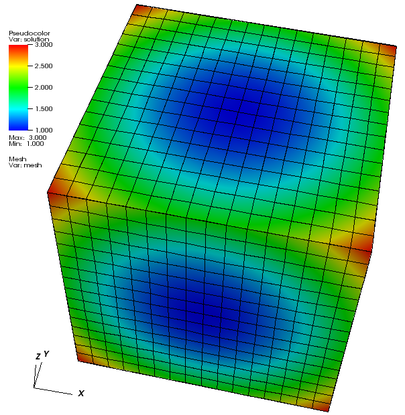
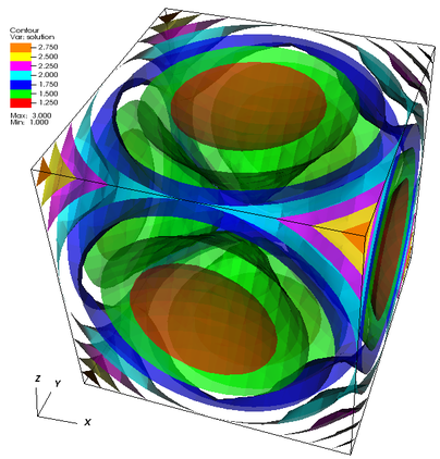
![$[-1,1]^3$](form_4709_dark.png)


 in 2d
in 2d 


![\begin{equation*}
F(\varepsilon) \dealcoloneq E(u+\varepsilon(v-u)),\quad\varepsilon\in\left[0,1\right],
\end{equation*}](form_4756_dark.png)


![\begin{eqnarray*}
&A U + B\Lambda = F,&\\
&[BU-G]_i \geq 0, \quad \Lambda_i \leq 0,\quad \Lambda_i[BU-G]_i = 0
\qquad \forall i.&
\end{eqnarray*}](form_4780_dark.png)


![\begin{eqnarray*}
&A U + B\Lambda = F,&\\
&U_i-B_{ii}^{-1}G_i \ge 0, \quad \Lambda_i \leq 0,\quad \Lambda_i[U_i-B_{ii}^{-1}G_i] = 0
\qquad \forall i\in{\cal S}.&
\end{eqnarray*}](form_4787_dark.png)
![\begin{equation*}
C([BU]_i,\Lambda_i) \dealcoloneq -\Lambda_i + \min\lbrace 0, \Lambda_i + c([BU]_i - G_i) \rbrace,
\end{equation*}](form_4788_dark.png)


![$\mathbf \sigma_t= \sigma \mathbf n - \mathbf \sigma_n \mathbf n
-= \sigma \mathbf n - [\mathbf n \cdot(\sigma \mathbf n)]\mathbf n$](form_4869_dark.png)


![$\mathbf \sigma_t= \sigma \mathbf n - \mathbf \sigma_n \mathbf n
+= \sigma \mathbf n - [\mathbf n \cdot(\sigma \mathbf n)]\mathbf n$](form_4853_dark.png)


 Find the primal-dual pair


![\begin{gather*}\mathcal{A}_{i+1} \dealcoloneq \lbrace p\in\mathcal{S}:\Lambda^i_p +
- c\left(\left[B^TU^i\right]_p - G_p\right) > 0\rbrace,\end{gather*}](form_4915_dark.png)


![$\mathbb{T} = [0,T_{\textrm{end}}]$](form_5256_dark.png)


![\[
\mathbf{x} = \boldsymbol{\varphi}(\mathbf{X},t) \, .
-\]](form_5048_dark.png)


![\[
\textrm{d}v = J(\mathbf{X},t)\; \textrm{d}V \, .
-\]](form_5054_dark.png)


![\[
\mathbf{F}
= (J^{1/3}\mathbf{I})\overline{\mathbf{F}}
\qquad \text{and} \qquad
\mathbf{b}
= (J^{2/3}\mathbf{I})\overline{\mathbf{F}}\,\overline{\mathbf{F}}^T
= (J^{2/3}\mathbf{I})\overline{\mathbf{b}} \, .
-\]](form_5058_dark.png)


![\[
\mathbf{l}(\mathbf{x},t)
\dealcoloneq \dfrac{\partial \mathbf{v}(\mathbf{x},t)}{\partial \mathbf{x}}
= \textrm{grad}\ \mathbf{v}(\mathbf{x},t) \, ,
-\]](form_5062_dark.png)


![\[
\mathbf{t}(\mathbf{x},t, \mathbf{n}) = \boldsymbol{\sigma}\mathbf{n} \, .
-\]](form_5065_dark.png)


![\[
\mathbf{T}(\mathbf{X},t, \mathbf{N}) = \mathbf{P}\mathbf{N} \, .
-\]](form_5068_dark.png)

![\[
\mathbf{t}\mathrm{d}a = \mathbf{T}\mathrm{d}A \, .
-\]](form_5069_dark.png)


![\[
\chi_{*}(\bullet)^{\text{cov}} \dealcoloneq \mathbf{F}^{-T} (\bullet)^{\text{cov}} \mathbf{F}^{-1}
\qquad \text{and} \qquad
\chi^{-1}_{*}(\bullet)^{\text{cov}} \dealcoloneq \mathbf{F}^{T} (\bullet)^{\text{cov}} \mathbf{F} \, .
-\]](form_5074_dark.png)


![\[
\chi_{*}(\bullet)^{\text{con}} \dealcoloneq \mathbf{F} (\bullet)^{\text{con}} \mathbf{F}^T
\qquad \text{and} \qquad
\chi^{-1}_{*}(\bullet)^{\text{con}} \dealcoloneq \mathbf{F}^{-1} (\bullet)^{\text{con}} \mathbf{F}^{-T} \, .
-\]](form_5076_dark.png)


![\[
\mathbf{S}
= 2 \dfrac{\partial \Psi(\mathbf{C})}{\partial \mathbf{C}} \, .
-\]](form_5079_dark.png)

![\[
\boldsymbol{\tau}
= 2 \dfrac{\partial \Psi(\mathbf{b})}{\partial \mathbf{b}} \mathbf{b}
= 2 \mathbf{b} \dfrac{\partial \Psi(\mathbf{b})}{\partial \mathbf{b}} \, .
-\]](form_5080_dark.png)


 first_vector_components = <
![$\Omega=[0,1]^2$](form_2794_dark.png)


![\[
Z = \{ \varphi: \varphi(x)=0 \}.
-\]](form_5319_dark.png)


![\begin{align*}
\int_0^L (\Delta \varphi_i) (\Delta \varphi_j)
=
\int_0^L
\frac 1h \left[\delta(x-x_{i-1}) - 2\delta(x-x_i) + \delta(x-x_{i+1})\right]
\frac 1h \left[\delta(x-x_{j-1}) - 2\delta(x-x_j) + \delta(x-x_{j+1})\right]
-\end{align*}](form_5368_dark.png)


 step-20 from the regular Laplace equation by introducing a second variable, we can here introduce a variable


 A generic interface for parallel cell-based finite element operator application by Martin Kronbichler and Katharina Kormann, Computers and Fluids 63:135–147, 2012, and the paper "Parallel finite element operator application: Graph partitioning and coloring" by Katharina Kormann and Martin Kronbichler in: Proceedings of the 7th IEEE International Conference on e-Science, 2011.


![$[-15,15]$](form_5117_dark.png)
![$[-15,15]$](form_5489_dark.png)


 regular input mesh
  output mesh

 regular input mesh
  wall-adapted output mesh


![$\Omega = [-1,1]^\text{dim} \setminus [0,1]^\text{dim}$](form_5560_dark.png)


 In 3D, the solution looks similar (see below). On the left you can see the solution and on the right we show a slice for


 MGTools::workload_imbalance(). This value, which will be denoted by


![$\Omega \dealcoloneq [-1,1]^d$](form_5678_dark.png)


![$[0,b]\times[0,b]$](form_5601_dark.png)


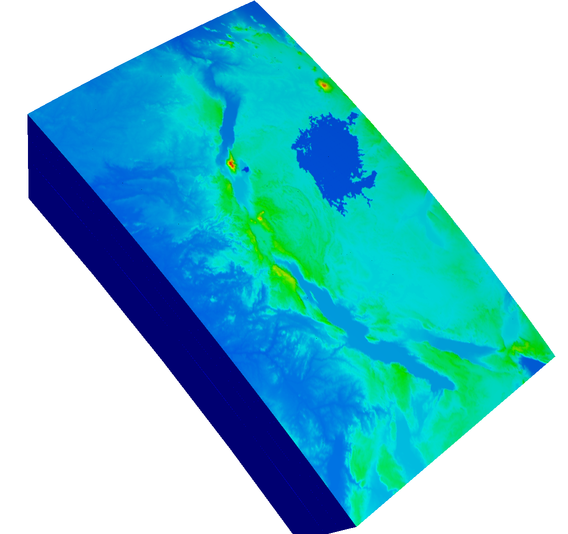
![$\hat U=[26,35]\times[-10,5]\times[-500000,0]$](form_5594_dark.png)


![$[-11.98333^\circ,6.983333^\circ]\times[25^\circ,35.98333^\circ]$](form_5682_dark.png)
![$[-6.983333^\circ,11.98333^\circ]$](form_5683_dark.png)


![$[-6.983333, 11.98333]$](form_5623_dark.png)
![$[-6.983333, 11.98333]$](form_5687_dark.png)
![$[25, 35.983333]$](form_5688_dark.png)

![$[0,2\pi]$](form_5690_dark.png)


![\[
\| u -u_h \|_0 + h ( \| u- u_h\|_1 + \|p - p_h \|_0)
\leq C h^{k+1} ( \|u \|_{k+1} + \| p \|_k )
\]](form_5727_dark.png)


![\[
\left(\int_\Omega e^{-\frac{r_k^2}{R^2}}\right)^{-1}
=
@@ -669,15 +669,15 @@
\]](form_5915_dark.png)


![\[
\nabla\psi(\mathbf x,t)\cdot \mathbf n=0 \qquad\qquad \forall \mathbf x\in\partial\Omega.
\]](form_5920_dark.png)

![\[
V(\mathbf x)
=
@@ -687,7 +687,7 @@
\end{cases}
\]](form_5921_dark.png)


 MatrixFree::cell_loop() that we used in


![\[
-\nabla \cdot (a \nabla u) = f.
\]](form_6029_dark.png)


![\[
V_h(\Omega) = \text{span} \{v_i\}_{i=1}^n
-\]](form_6064_dark.png)


![\[
-\omega^2\rho \xi u_m - \partial_n \left(\frac{\xi c_{mnkl}}{2s_n s_k} \partial_k u_l
+ \frac{\xi c_{mnkl}}{2s_n s_l} \partial_l u_k\right) = f_m
@@ -211,13 +211,13 @@
+ \beta_{mnkl}\partial_l u_k\right) = f_m
\]](form_6202_dark.png)


![$\Omega =
-[-1,\,1]\times[-1,\,1]\backslash B_{0.3}(0)$](form_6267_dark.png)

![$\boldsymbol{\beta} =
-[-\sin(\pi/6),\,\cos(\pi/6)]$](form_6269_dark.png)


![\begin{align*}
(x,y) = (1-\eta) \big[(1-\xi) (x_0,y_0) + \xi (x_1,y_1)\big] +
\eta \mathbf{c}_3(\xi),
\end{align*}](form_6285_dark.png)


![$[-1, 1]$](form_738_dark.png)


![$F'(u_h^n)[\,\cdot\,]\colon\mathbb{R}^N\to\mathbb{R}^N$](form_6327_dark.png)


![$\lambda\in[0,6]$](form_6357_dark.png)


![$\lambda\in[0,6]$](form_6345_dark.png)


![\[
\left(\mathbf{v}, \frac{\partial \mathbf{w}}{\partial t}\right)_{K}
+ \left(\mathbf{v}, \nabla \cdot \mathbf{F}(\mathbf{w})\right)_{K} =
\left(\mathbf{v},\mathbf{G}(\mathbf w)\right)_{K}.
-\]](form_6365_dark.png)


![$[\![\mathbf{w}]\!]$](form_6437_dark.png)


![$[\![\mathbf{w}]\!]$](form_6377_dark.png)


![\[
\hat{\mathbf{F}}(\mathbf{w}^-,\mathbf{w}^+) =
\frac{s^\mathrm{p} \mathbf{F}(\mathbf{w}^-)-s^\mathrm{n} \mathbf{F}(\mathbf{w}^+)}
{s^\mathrm p - s^\mathrm{n} } +
\frac{s^\mathrm{p} s^\mathrm{n}}{s^\mathrm{p}-s^\mathrm{n}}
\left[\mathbf{w}^--\mathbf{w}^+\right]\otimes \mathbf{n^-}.
-\]](form_6386_dark.png)


![\[
\mathbf{w}^+ = \begin{pmatrix} \rho_\mathrm{D}(t)\\
(\rho \mathbf u)_{\mathrm D}(t) \\ E_\mathrm{D}(t)\end{pmatrix} \quad
\text{(Dirichlet)},
-\]](form_6392_dark.png)


![\[
\frac{d \textbf{x}_i}{dt} =\textbf{u}(\textbf{x}_i)
-\]](form_6512_dark.png)

![\[
\textbf{x}_{i}^{n+1} = \textbf{x}_{i}^{n} + \Delta t \; \textbf{u}(\textbf{x}_{i}^{n})
-\]](form_6515_dark.png)


![$\textbf{u}=[u,v]^T$](form_6349_dark.png)

![$\textbf{u}=[u,v]^T$](form_6520_dark.png)


![$\textbf{u} = [\rho, \textbf{m}^\top,E]^{\top}$](form_6589_dark.png)


![$\textbf{u} = [\rho, \textbf{m}^\top,E]^{\top}$](form_6532_dark.png)


![$\gamma \in (1,5/3]$](form_6599_dark.png)
![$\gamma \in (1,5/3]$](form_6540_dark.png)


![\begin{align}
\mathcal{B} = \big\{ \textbf{u} =
[\rho, \textbf{m}^\top,E]^{\top} \in \mathbb{R}^{d+2} \, \big |
\
@@ -201,81 +201,81 @@
\
s(\mathbf{u}) \geq \min_{x \in \Omega} s(\mathbf{u}_0(\mathbf{x}))
\big\}.
-\end{align}](form_6550_dark.png)


![\[
E = \| {\mathbf e} \| = \left( \sum_K e_K^2 \right)^{1/2}
-\]](form_6693_dark.png)


![\[
u = g_1
-\]](form_6696_dark.png)
![\[
{\mathbf n}\cdot \nabla u = g_2
-\]](form_6697_dark.png)


![\[
{(\nabla v, \nabla u)}_\Omega + {(v,u)}_\Omega
=
{(v,f)}_\Omega + {(v,g_2)}_{\Gamma_2}
-\]](form_6705_dark.png)


![\[
\bar u(\mathbf x) =
\sum_{i=1}^3 \exp\left(-\frac{|\mathbf x-\mathbf x_i|^2}{\sigma^2}\right)
-\]](form_6711_dark.png)


![\[
\dot{E}_{0}
= \mathbf{P}^{\text{tot}} : \dot{\mathbf{F}}
+ \boldsymbol{\mathbb{H}} \cdot \dot{\boldsymbol{\mathbb{B}}}
+ \mathbb{E} \cdot \dot{\mathbb{D}}
- \nabla_{0} \cdot \mathbf{Q}
+ R_{0} .
-\]](form_6791_dark.png)


![\[
\mathbf{P}^{\text{tot}} : \dot{\mathbf{F}}
+ \boldsymbol{\mathbb{H}} \cdot \dot{\boldsymbol{\mathbb{B}}}
+ \mathbb{E} \cdot \dot{\mathbb{D}}
@@ -208,26 +208,26 @@
- \dot{E}_{0}
- \frac{1}{\theta} \nabla_{0} \theta \cdot \mathbf{Q}
\geq 0 .
-\]](form_6795_dark.png)


![\[
\mathcal{D}_{\text{int}}
= \mathbf{P}^{\text{tot}} : \dot{\mathbf{F}}
+ \boldsymbol{\mathbb{H}} \cdot \dot{\boldsymbol{\mathbb{B}}}
@@ -235,104 +235,104 @@
- \dot{\theta} \eta_{0}
- \dot{\psi}^{*}_{0} \left( \mathbf{F}, \boldsymbol{\mathbb{B}}, \mathbb{D}, \theta \right)
\geq 0 .
-\]](form_6799_dark.png)


![\[
\tilde{\psi}_{0} \left( \mathbf{F}, \mathbf{F}_{v}^{i}, \boldsymbol{\mathbb{H}} \right)
= \psi^{*}_{0} \left( \mathbf{F}, \mathbf{F}_{v}^{i}, \boldsymbol{\mathbb{B}} \right)
- \boldsymbol{\mathbb{H}} \cdot \boldsymbol{\mathbb{B}} .
-\]](form_6803_dark.png)


 partial derivatives
![\[
\frac{\partial f\left(x, y\right)}{\partial x}
= \frac{d f\left(x, y\right)}{d x} \Big\vert_{y} .
-\]](form_6811_dark.png)


![\[
\mathbf{S}^{\text{tot}}
= \mathbf{S}^{\text{tot}} \left( \mathbf{C}, \mathbf{C}_{v}^{i}, \boldsymbol{\mathbb{H}} \right)
\dealcoloneq 2 \frac{\partial \psi_{0} \left( \mathbf{C}, \mathbf{C}_{v}^{i}, \boldsymbol{\mathbb{H}} \right)}{\partial \mathbf{C}} , \\
\boldsymbol{\mathbb{B}}
= \boldsymbol{\mathbb{B}} \left( \mathbf{C}, \mathbf{C}_{v}^{i}, \boldsymbol{\mathbb{H}} \right)
\dealcoloneq - \frac{\partial \psi_{0} \left( \mathbf{C}, \mathbf{C}_{v}^{i}, \boldsymbol{\mathbb{H}} \right)}{\partial \boldsymbol{\mathbb{H}}} .
-\]](form_6816_dark.png)


![\[
F(U)_i \dealcoloneq
\int\limits_{\Omega}\nabla \varphi_i \cdot \left[ \frac{1}{\sqrt{1+|\nabla
u|^{2}}} \nabla u \right] \, dV ,
-\]](form_6950_dark.png)


![\[
F(U)_i^K \dealcoloneq
\int\limits_K\nabla \varphi_i \cdot \left[ \frac{1}{\sqrt{1+|\nabla
u|^{2}}} \nabla u \right] \, dV ,
-\]](form_6952_dark.png)


![\[
F(U)_i^K \dealcoloneq
\int\limits_K\nabla \varphi_i \cdot \left[ \frac{1}{\sqrt{1+\left|
\sum_{j'}^{n_\textrm{dofs}} U_{j'} \nabla \varphi_{j'}\right|^{2}}}
\left(\sum_{j''}^{n_\textrm{dofs}} U_{j''} \nabla \varphi_{j''}\right)\right] \, dV.
-\]](form_6955_dark.png)


![\[
\jump{v} = v^0 - v^1
-\]](form_6984_dark.png)


![$\sum_{f\in \partial K \cap \partial \Omega}
+ \sigma \left\| [ u_h-g_D ] \right\|_f^2 $](form_7011_dark.png)


![\[
u_\text{hp}(x) = \sum c_i \varphi_i(x)
-\]](form_7023_dark.png)


![\[
u_\text{hp}(x) = \sum l_k P_k(x).
-\]](form_7024_dark.png)


![\[
l_k = \int_K u_\text{hp}(x) P_k(x) dx.
-\]](form_7026_dark.png)

![\[
\int_K P_i(x) P_j(x) dx = \det(J_K) \, \delta_{ij}
-\]](form_7027_dark.png)


![\[
\int_K u_\text{hp}(x) P_k(x) dx
= \det(J_K) \int_{\hat{K}} u_\text{hp}(F_K(\hat{x})) P_k(F_K(\hat{x})) d\hat{x}.
-\]](form_7030_dark.png)


![\[
\int_K P_i(x) \varphi_j(x) dx
= \det(J_K) \int_{\hat{K}} P_i(F_K(\hat{x})) \varphi_j(F_K(\hat{x})) d\hat{x}
= \det(J_K) \int_{\hat{K}} \hat{P}_i(\hat{x}) \hat{\varphi}_j(\hat{x}) d\hat{x}
\dealcoloneq \det(J_K) \, C_{ij}
-\]](form_7032_dark.png)

![\[
\det(J_K) \, \mathbb{I} \, \mathbf{l} = \det(J_K) \, \mathbf{C} \, \mathbf{c}
-\]](form_7033_dark.png)


![\[
\exists C,\sigma > 0 : \quad \forall k \in \mathbb{N}_0 : \quad |l_k|
\leq C \exp\left( - \sigma k \right) .
-\]](form_7035_dark.png)

![\[
\ln(|l_k|) \sim \ln(C) - \sigma k .
-\]](form_7036_dark.png)


![\[
u_\text{sol} = r^{2/3} \sin(2/3 \varphi).
-\]](form_7040_dark.png)


 step-15 uses a Newton method, and Newton's method works by repeatedly solving a linearized problem for an update


![$\Omega=[0,S_\text{max}]$](form_6886_dark.png)


![$\Omega=[0,S_\text{max}]$](form_7093_dark.png)


![\begin{align*}
0=&-\frac{V^n(S)-V^{n-1}(S)}{k_n} \\
&+\frac{\sigma^2S^2}{2}\left[(1-\theta)\frac{d^2V^{n-1}(S)}{dS^2} + \
\theta \frac{d^2V^{n}(S)}{dS^2}\right] \\
&+rS\left[(1-\theta)\frac{dV^{n-1}(S)}{dS} + \
\theta\frac{dV^{n}(S)}{dS}\right] \\
&-r\left[(1-\theta)V^{n-1}(S) + \theta V^n(S)\right]
-\end{align*}](form_7108_dark.png)


![\begin{align*}
0=&-\int_0^{S_\text{max}}\phi_i(S)\left[V^n(S)-V^{n-1}(S)\right]dS \\
&+k_n\int_0^{S_\text{max}}\phi_i(S)\left[\frac{\sigma^2S^2}{2} \
\left[(1-\theta)\frac{d^2V^{n-1}(S)}{dS^2} + \
@@ -209,12 +209,12 @@
+ \theta\frac{dV^{n}(S)}{dS}\right]\right]dS \\
&-k_n\int_0^{S_\text{max}}\phi_i(S)\left[r\left[(1-\theta)V^{n-1}(S)\
+ \theta V^n(S)\right]\right]dS
-\end{align*}](form_7111_dark.png)

![$k_n\left[-r(1-\theta)\textbf{M}V^{n-1} - \theta r\textbf{M}V^n\right]$](form_6906_dark.png)


![$k_n\left[-r(1-\theta)\textbf{M}V^{n-1} - \theta r\textbf{M}V^n\right]$](form_7113_dark.png)


![\begin{align*}
&k_n\int_0^{S_\text{max}}\phi_i(S)\left[\frac{\sigma^2S^2}{2}
\left[(1-\theta)\
\frac{d^2V^{n-1}(S)}{dS^2} + \
@@ -261,19 +261,19 @@
-(1-\theta)\frac{1}{2}\sigma^2\textbf{D}V^{n-1} \
-\theta\sigma^2\textbf{B}V^{n}
-\theta\frac{1}{2}\sigma^2\textbf{D}V^{n}\right]
-\end{align*}](form_7119_dark.png)


![\begin{align*}
&k_n\int_0^{S_\text{max}}\phi_i(S)\left[rS\left[(1-\theta)
\frac{dV^{n-1}(S)}{dS} +\
\theta\frac{dV^{n}(S)}{dS}\right]\right]dS \\
&= k_n\left[-(1-\theta)r\textbf{M}V^{n-1} -(1-\theta)r\textbf{A}V^{n-1}\
-\theta r\textbf{M}V^n -\theta r\textbf{A}V^n\right]
-\end{align*}](form_7124_dark.png)


![\[
\text{minimize}\| \boldsymbol{\sigma} (\mathbf{u}) \|_\infty
-\]](form_7143_dark.png)


![\[
-
\text{div}\,
({\mathbf C} \varepsilon(\mathbf u))
=
\mathbf f,
-\]](form_7243_dark.png)


![\[
c_{ijkl}
=
\lambda \delta_{ij} \delta_{kl} +
\mu (\delta_{ik} \delta_{jl} + \delta_{il} \delta_{jk}).
-\]](form_7247_dark.png)


![\[
\Phi_i({\mathbf x}) = \varphi_{\text{base}(i)}({\mathbf x})\ {\mathbf e}_{\text{comp}(i)},
-\]](form_7255_dark.png)


![\[
\phi_i = \varphi_{\text{base}(i)}
-\]](form_7267_dark.png)


![\[
a({\mathbf u}_h, {\mathbf v}_h) = ({\mathbf f}, {\mathbf v}_h)
\qquad
\forall {\mathbf v}_h.
-\]](form_7271_dark.png)


![\[
\frac{\partial}{\partial t} \rho + \nabla\cdot\mathbf{J}_a = 0
\text{ and }
\frac{\partial}{\partial t} \rho_m + \nabla\cdot\mathbf{M}_a = 0.
-\]](form_7294_dark.png)

![\[
\mathbf{F}(\mathbf{x},t) = \text{Re}\{e^{-i\omega
t}\tilde{\mathbf{F}}(\mathbf{x})\},
-\]](form_7295_dark.png)


![\[
+<p>Graphene is a two-dimensional carbon allotrope with a <em>single</em> atom layer that is arranged in a honeycomb lattice <b>[Geim2004]</b>. Due to its atomic thickness it is an example of a so-called 2D material: Compared to the other spatial dimensions (where graphene samples can reach up to several centimeters) the atomistic thickness of graphene typically ranges around 2.5 ångstrom ( <picture><source srcset=](form_7138_dark.png)


![\[
\mathbf{J}^\Sigma=\sigma^\Sigma\,\mathbf{E}_T
-\]](form_7304_dark.png)


![\begin{align*}
\mathbf{\nu} \times \left[(\mu^{-1}\mathbf{H})^+ - (\mu^{-1}\mathbf{H})^-\right]|_{\Sigma}
&= \sigma^{\Sigma}\left[(\mathbf{\nu}\times \mathbf{E}\times \mathbf{\nu})\right]|_{\Sigma},
\\
\mathbf{\nu} \times \left[\mathbf{E}^+ - \mathbf{E}^-\right]|_{\Sigma} &= 0.
-\end{align*}](form_7308_dark.png)


![\[
\mathbf{J}_a = J_0 \mathbf{e}_i\delta(x-a)
-\]](form_7315_dark.png)

![\[
\mu_r = \frac{1}{\mu_0}\mu
\text{ and }
\varepsilon_r = \frac{1}{\varepsilon_0}\varepsilon.
-\]](form_7316_dark.png)

![\[
\begin{align*}
\hat{x} = k_0x, &\qquad
\hat{\nabla} = \frac{1}{k_0}\nabla,\\
@@ -236,15 +236,15 @@
\hat{\mathbf{J}}_a = \frac{1}{J_0}\mathbf{J}_a,&\qquad
\hat{\mathbf{M}}_a = \frac{k_0}{\omega\mu_0 J_0}\mathbf{M}_a.
\end{align*}
-\]](form_7318_dark.png)


![\[
\nabla \times (\mu_r^{-1}\nabla\times\mathbf{E}) - \varepsilon_r \mathbf{E}
= i\mathbf{J}_a - \nabla\times (\mu_r^{-1}\mathbf{M}_a).
-\]](form_7323_dark.png)


![\[
\int_\Omega (\mu_r^{-1}\nabla\times\mathbf{E})\cdot (\nabla\times\bar{\varphi})\;\text{d}x
- \int_\Omega \varepsilon_r\mathbf{E} \cdot \bar{\varphi}\;\text{d}x
- \int_\Sigma [\nu \times (\mu_r^{-1}\nabla\times\mathbf{E} +
@@ -277,32 +277,32 @@
\mu^{-1}\mathbf{M}_a)) \cdot \bar{\varphi}_T\;\text{d}o_x =
i\int_\Omega \mathbf{J}_a \cdot \bar{\varphi}\;\text{d}x
- \int_\Omega \mu_r^{-1}\mathbf{M}_a \cdot (\nabla \times \bar{\varphi})\;\text{d}x.
-\]](form_7326_dark.png)
![$[\cdot]_{\Sigma}$](form_7176_dark.png)

![$[\cdot]_{\Sigma}$](form_7327_dark.png)
![\[
\mathbf{F}_T = (\mathbf{\nu}\times \mathbf{F})\times\mathbf{\nu}
\text{ and }
[\mathbf{F}]_{\Sigma}(\mathbf{x}) = \lim\limits_{s\searrow 0}(\mathbf{F}(\mathbf{x}+s\mathbf{\nu})-\mathbf{F}(\mathbf{x}-s\mathbf{\nu}))
-\]](form_7328_dark.png)


![\[
\nu\times\mathbf{H}+\sqrt{\mu_r^{-1}\varepsilon_r}\mathbf{E}=0\qquad x\in\partial\Omega
-\]](form_7330_dark.png)


![\[
\int_{\Omega}D^2u:D^2v = \int_{\Omega}fv \qquad \forall \, v\in H_0^2(\Omega),
-\]](form_7385_dark.png)


![\[
\mathbb{V}_h\dealcoloneq\left\{v_h\in L^2(\Omega): \,\, v_h|_K\circ F_{K}\in\mathbb{Q}_k \quad \forall \, K \in\mathcal{T}_h \right\},
-\]](form_7393_dark.png)


![$H_h(v_h)\in\left[L^2(\Omega)\right]^{d\times d}$](form_7289_dark.png)


![$H_h(v_h)\in\left[L^2(\Omega)\right]^{d\times d}$](form_7402_dark.png)

![$r_e:[L^2(e)]^d\rightarrow[\mathbb{V}_h]^{d\times d}$](form_7404_dark.png)
![$b_e:L^2(e)\rightarrow[\mathbb{V}_h]^{d\times d}$](form_7405_dark.png)
![\[
r_e\left(\boldsymbol{\phi}\right) \in [\mathbb{V}_h]^{d\times d}: \,
\int_{\Omega} \tau_h : r_e\left(\boldsymbol{\phi}\right) = \int_e\average{\tau_h}\mathbf{n}_e\cdot\boldsymbol{\phi} \qquad \forall \, \tau_h\in [\mathbb{V}_h]^{d\times d}
-\]](form_7406_dark.png)


![$H_h:\mathbb{V}_h\rightarrow\left[L^2(\Omega)\right]^{2\times 2}$](form_7410_dark.png)
![\[
H_h(v_h) \dealcoloneq D_h^2 v_h -R_h(\jump{\nabla_h v_h})+B_h(\jump{v_h}) \dealcoloneq D_h^2 v_h - \sum_{e\in\mathcal{E}_h}r_e\left(\jump{\nabla_h v_h}\right)+\sum_{e\in\mathcal{E}_h}b_e\left(\jump{v_h}\right).
-\]](form_7411_dark.png)


![$\tau\in [C_0^{\infty}(\Omega)]^{d\times d}$](form_7414_dark.png)
![\[
\int_{\Omega}H_h(v_h):\tau\longrightarrow \int_{\Omega}D^2v:\tau \qquad \mbox{as } \,\, h\rightarrow 0
-\]](form_7415_dark.png)


![\[
\int_{\Omega}D^2v:\tau = -\int_{\Omega}\nabla v\cdot \mbox{div}(\tau) = \int_{\Omega}v \mbox{ div}(\mbox{div}(\tau))
-\]](form_7419_dark.png)

![\[
\int_K v_h \mbox{ div}(\mbox{div}(\tau)) = -\int_K \nabla v_h\cdot \mbox{div}(\tau) + \int_{\partial K} v_h \mbox{ div}(\tau)\cdot \mathbf{n}_K =\int_K D^2v_h:\tau - \int_{\partial K}\nabla v_h\cdot (\tau\mathbf{n}_K) + \int_{\partial K} v_h \mbox{ div}(\tau)\cdot \mathbf{n}_K,
-\]](form_7422_dark.png)


![\[
\int_{\Omega} v_h \mbox{ div}(\mbox{div}(\tau)) = \int_{\Omega} D_h^2v_h:\tau - \sum_{e\in\mathcal{E}_h}\int_e\jump{\nabla_h v_h}\cdot \average{\tau}\mathbf{n}_e + \sum_{e\in\mathcal{E}_h}\int_e v_h \average{\mbox{div}(\tau)}\cdot \mathbf{n}_e
-\]](form_7424_dark.png)


![$[\mathbb{V}_h\cap H_0^1(\Omega)]^{d\times d}$](form_7426_dark.png)


![\[
A_h(u_h,v_h)\dealcoloneq a_h(u_h,v_h)+j_h(u_h,v_h) = F_h(v_h) \qquad \forall \, v_h\in\mathbb{V}_h,
-\]](form_7431_dark.png)


![\[
A\boldsymbol{U} = \boldsymbol{F},
-\]](form_7437_dark.png)


![\[
A_{ij}\dealcoloneq A_h(\varphi_j,\varphi_i) \quad \text{and} \quad F_i\dealcoloneq F_h(\varphi_i), \qquad 1\leq i,j \leq N_h.
-\]](form_7440_dark.png)


![\[
\|v_h\|_{H_h^2(\Omega)}^2\dealcoloneq\|D_h^2v_h\|_{L^2(\Omega)}^2+\sum_{e\in\mathcal{E}_h}h_e^{-1}\|\jump{\nabla_h v_h}\|_{L^2(e)}^2+\sum_{e\in\mathcal{E}_h}h_e^{-3}\|\jump{v_h}\|_{L^2(e)}^2
- \]](form_7442_dark.png)


![$[L^2(\Omega)]^{2\times 2}$](form_7354_dark.png)


![$[L^2(\Omega)]^{2\times 2}$](form_7446_dark.png)


![\begin{equation*}
g_h(u_h,v_h) = \gamma_A \sum_{F \in \mathcal{F}_h} (h_F [\partial_n u_h], [\partial_n v_h])_F.
\end{equation*}](form_7582_dark.png)


![$[-1, 1]^{\text{dim}}$](form_7597_dark.png)


![\[
(\beta \cdot \nabla u_h, v_h + \delta \beta\cdot\nabla v_h)_\Omega
@@ -194,7 +194,7 @@
(\varphi_i, \beta\cdot {\mathbf n} \varphi_j)_{\partial\Omega_-},
\]](form_7613_dark.png)


![\[
U^T A = F^T,
\]](form_7620_dark.png)


![\begin{eqnarray*}
\Omega &=& [-1,1]^d \\
\beta({\mathbf x})
@@ -347,15 +347,15 @@
\]](form_7638_dark.png)

![\[
\frac{{\mathbf y}_{KK'}^T}{|{\mathbf y}_{KK'}|} \nabla u
\approx
\frac{u(K') - u(K)}{|{\mathbf y}_{KK'}|},
\]](form_7647_dark.png)


![\[
\underbrace{
\left(\sum_{K'} \frac{{\mathbf y}_{KK'} {\mathbf y}_{KK'}^T}
@@ -367,7 +367,7 @@
\frac{u(K') - u(K)}{|{\mathbf y}_{KK'}|}.
\]](form_7651_dark.png)


